Abstract
This paper presents an agent-based simulation model for end-of-life product flow analysis in recuperation and recycling supply networks that focuses on individual consumer behaviors. The simulation model is applied to a deposit-return program on wine bottles that could be developed in the province of Quebec. Canadian data was used to calibrate and validate the model. A series of experiments was then conducted with three artificial populations to analyse how they would react to several implementation scenarios of this end-of-life product flow strategy. The results suggest that the distance to the nearest depot is an important decision factor, but less predominant than the ownership of a private vehicle and the deposit value. The results also indicate that the use of agent-based modeling combined with the theory of planned behavior (TPB) can produce modular behavior models, that are intuitive and simple, to better understand consumer-behavior-driven supply chains. Such models can be used to give insights to decision-makers and policy-makers about the potential performance of end-of-life product flows strategies and further facilitate efficient resource management.
1. Introduction
With Earth Overshoot Day getting earlier every year, it is more important than ever before to manage Earth’s resources in effective ways. Considering that over 1.47 billion tons of municipal solid waste is generated each year [1], and only 15% out of the 84% collected waste is recycled, it comes as no surprise that actual municipal waste management practices are not sustainable. With resources scarcity lurking, the application of circular economy (CE) models to end-of-life (EOL) product flow networks can offer great opportunities to strive towards a more sustainable future.
In this context of new business and product flow models, the ability to compare both economically and environmentally multiple product flow strategies is undoubtedly relevant to decision-makers willing to progress towards CE goals [2,3]. A difficult aspect of the analysis of new strategy introduction is the human factor. It is indeed difficult to predict how people may react when faced with various options, which, in turn, makes it difficult to assess technical feasibility and profitability. In order to address this issue, computer simulation offers a compelling analytical approach since it enables both macro and micro modeling capabilities in a risk-free environment [4]. This paper proposes a simulation model of consumer behavior for end-of-life product flow to work towards finding more sustainable end-of-life product flow strategies. It is applied to a case study of Quebec’s wine bottle potential deposit-return scheme that is currently being looked at by policy-makers. The simulation model can be used to estimate the percentages of products that are sent in each end-of-life option according to various parameters such as the deposit value, the consumer-to-depot maximum distance, and the proportion of the population owning a vehicle. The model is calibrated and validated with various independent data sources. Merging these data sources in one single model enables the emergence of behavior tendencies that would not be observable without the consumer behavior simulation model.
1.1. Solid Waste Management
Waste management is a sensitive field of research as it concerns everybody; each citizen living in the developed world uses and pays for municipal waste management systems (MWMS). Over the past decades, many strategies and policies have been implemented all over the world, such as high recycling targets or household-level user fees, to maximise the benefits and minimise the costs of municipal solid waste management [5]. To facilitate the analysis and development of these programs and policies, researchers have decomposed and estimated the costs of MWMS [6,7]. However, the complexity of the MWMS comes from the dichotomy between its two complementary aspects: the economic costs and the environmental impacts of the strategies [2,3]. Many researchers completed multiple assessments of MWMS environmental impacts [8,9], from single stream collection versus the separation of recyclables [10], to specific products [11], such as polyethylene terephthalate (PET) and glass bottles [12,13]. However, the complex link between consumers behaviors and MWMS mass flows remains a significant and sensitive element of these assessment studies. In order to address this issues, [14] have successfully developed a mathematical model to forecast municipal solid waste generation based on prognostic tools and regression analysis. Although such models are well suited to assess MWMS in stable conditions, they can hardly capture social impacts such as incentives, media campaigns or social interactions between households.
1.2. Behavioral Theories
There is a growing literature studying pro-environmental behaviors, such as recycling, using theoretical models [15,16], empirical data [17,18,19,20,21] or a combination of both [22,23,24,25,26,27]. Although there are several types of models, the theory of planned behavior (TPB) [28] seems to be the most frequently used here [29,30,31,32,33]. The model presented in this paper exploits this theoretical model, which is discussed hereafter.
1.3. Simulation of Waste Management Operations
The first models developed for household waste management were stochastic mathematical models created to predict the performance of a newspaper recycling strategy [34] and to provide a proof-of-concept for the simulation of a complex artificial society composed of individual households with waste management behaviors [35].
After the popularization of agent-based modeling and simulation (ABMS) [36], a new generation of model began to appear. Particularly used to study the diffusion of innovations, which share some similarities with recycling behavior adoption, these agent-based models were now able to capture the sophisticated effects of human interactions and their emergent phenomena [37]. Largely used among behaviorists, the TPB also made its way into ABMS [38]. An environmental innovation diffusion model was developed by [39], while [40] simulated pro-environmental farming practices diffusion. More recently, [41] used structural equation modeling within the TPB framework to predict household recycling outcomes and [42] simulated the emergence of self-organized industrial symbiosis relations.
ABMS is also used for multi-objective analyses. For example, a large-scale simulation model was developed to compare single-stream and dual-stream solid waste management alternatives in the state of Florida, US [43]. Another example is the model of [44], in which they show how to couple ABMS with other modeling methods in the context of life-cycle assessments.
2. Objective and Methodology
This paper proposes a simulation model for EOL product flow analysis in MWMS that focuses on individual consumer behaviors. In the model, autonomous entities known as agents purchase, consume, and eventually discard products in a way that is similar to how real consumers, from specific populations, would behave. With an artificial population, it becomes possible to estimate each proportion of materials diverted to every end-of-life option. Having the ability to simulate a whole population of diverse consumers enables the study and analysis of new waste management strategies and policies without having to implement them in the real world, thus minimizing the risks of failure and unexpected drawbacks. ABMS was chosen for this paper’s model because it facilitates the implementation of key concepts, such as autonomous and individual decision-making across a population of various types of consumers as well as complex social interactions that will soon be implemented into the model [36]. This consumer behavior model is applied to the study case of Quebec’s wine bottles whereby a deposit scheme would be implemented as a new municipal waste management policy.
3. The Model
First and foremost, since the point of interest in the system is where the wine bottles are diverted to one of each EOL options, this model is limited to the consumers and their decisions. A mathematical model of the consumer behavior decision process was developed to estimate the proportions of bottles sent towards the landfills and recycling facilities through the choices that consumers make; whether it is to put the bottles in the waste containers, the curbside container (also called blue bin) for collection, or to bring them back to return centers. As shown in Figure 1, bottles are purchased at a liquor store, then stored until they are emptied and eventually discarded. Depending on the consumers’ decisions, the bottles could end up either in landfills or recycling centers. It is assumed that the decisions are made for each individual bottle and that the process through the studied system is cyclic.
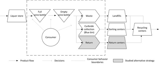
Figure 1.
How wine bottles go from the store to the landfills or recycling centers.
3.1. Behavior and Decision-Making
In the theory of planned behavior, inputs are generally categorized and gathered into constructs. These theoretical artifacts are usually a combination of factors affecting the output of the model that have been, or could be, empirically validated [45]. In his original TPB framework, [28] suggested that behavior is influenced by intentions and perceived behavioral control (PBC), while intention would be defined by the constructs of attitude, subjective norm and PBC. The proposed model uses the same key concepts, plus an incentive construct, as shown in Figure 2.
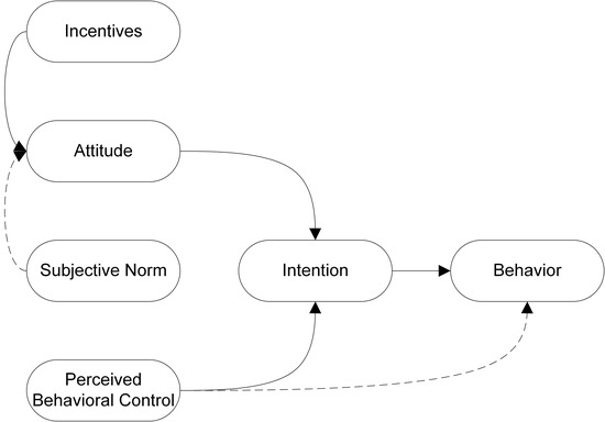
Figure 2.
Modified theory of planned behavior (TPB).
In the proposed model, Equations (1) and (2) show how behavior is calculated based on the TPB decision model. Here, i stands for the unique identification of each agent, b stands for the different behaviors, and t stands for the simulation time steps, which in this case are weeks. If an agent has an empty wine bottle, the calculation is done for each individual behavior, and the one with the highest Behaviori,t,b value is performed by the agent. If there are equal maximum behavior values, the performed behavior is randomly selected.
In the existing literature, whether it is in technology diffusion [39,40,46] or recycling [34,35,38], the simulated behavior always depicts binary decisions. In the first case, it is “adopt or don’t adopt”, where in the second case it is “recycle or don’t recycle”. Thus, developing specific equations for each behavior in the model enables the analysis of complex situations that have more than two possible behaviors without using thresholds.
Behaviori,t,b = Intentioni,t,b
Intentioni,t,b = Attitudei,t,b + PBCi,t,b(intention)
3.2. Attitude: Opinions and Incentives
Besides being influenced by subjective norms, which will be developed in the next iteration of this paper’s model, Attitudei,t,b is primarily defined by opinions (OVi,t,b) and incentives (IVb). The core aspect of the model, Opinions, represents how agents perceive each behavior on an environmental standpoint. As for Incentives, [15,47] supports the hypothesis that measures, such as deposits, can alter the perception of consumers toward environmental friendly behaviors. Therefore, it was implemented alongside Opinions, rather than as a distinct construct.
Attitude, used in Equation (2), is calculated using Equation (3). OVi,t,b and IVb are the two variables respectively corresponding to the agents’ opinions and the incentives. Ranging from 0 to 1, γ is the relative importance of OVi,t,b over IVb. This parameter is there to reflect the differences in consumers’ appreciation towards incentives. For example, a consumer who is not pro-environmental may be tempted to return their bottles solely for the deposit, while a pro-environmental consumer could be indifferent to the incentives. Specific to the population studied, γ follows a normal distribution that must be calibrated to fit a specific population or could be used to discover emergent population characteristics.
Attitudei,t,b = γ × OVi,t,b + (1 − γ) × IVb
An interesting feature of the proposed model is that it offers the possibility to have a continuous spectrum for environmental concerns (EC)—instead of a discrete categorisation of agents—while also keeping the notion of population segmentation that is often used in surveys. To do so, the model uses fuzzy logic to model a continuous form of membership of agents to segments. In other words, this framework enables the population to be segmented into 3 EC categories in a fuzzy manner: negative, neutral, and positive, as shown in Figure 3.
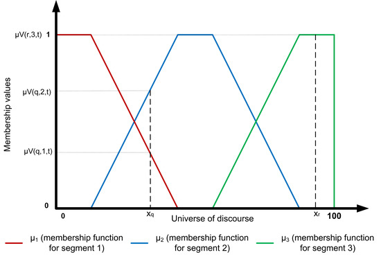
Figure 3.
Fuzzy logic membership functions with 3 segments.
The segments S do not directly depict the environmental concerns of agents towards a specific behavior. Instead, they are rather artifacts created to categorise and group together agents with homogenous interests, just as opinions are shared in political parties for example. Politicians can have slightly varying point of views yet share the same core values. Therefore, this division lets each segment have a relative attitude towards each behavior without encasing them into discrete opinion values.
As illustrated in Figure 3, every segment has a membership function µs that delineates the shape of the segment. The universe of discourse (UOD) X, referring to environmental concerns, has values of xi,t ranging continuously from 0 to 100. The shapes seamlessly blend into one another, creating smooth transitions between the segments.
Agents can be members of a single segments, or partially part of two segments. Within the UOD, each value of X has three corresponding membership values, ranging from 0 to 1. In the fuzzy logic approach, the sum of all the membership values µVi,s,t must always be equal to 1 for all the possible values of X in the UOD. For example, agent q in Figure 3 is a member of both segments 1 and 2 with his membership values being respectively 0.4 and 0.6. On the other hand, agent r is only part of segment 3, with his membership values being equal to 1 while µVr,1,t and µVr,2,t are both equal to 0.
Below is Equation (4) that defines an agents’ OVi,t,b according to their membership values and the segment’s opinion values matrix (SOVM). Calculated for all the behaviors, it is the summation of the agents’ membership values µVi,s,t multiplied by the corresponding values in the SOVM.
OVi,t,b = ∑sϵS[µVi,s,t × SOVb,s]
The SOVM, shown below, represents the distinct opinion values of the segments for all three behaviors. This matrix will be used with the membership values µVi,s,t of each segment to calculate agents.
Finally, for the IVb values, the only incentive in this paper’s case study is the deposit on the bottles. IVb is implemented in the model as a discrete value where one unit equals one cent.
3.3. The Perceived Behavioral Control
The PBC can be described as how consumers perceive themselves capable of accomplishing a specific behavior with their current capabilities and factors such as available resources or any socio-demographic characteristic. In the current model, only vehicle ownership and the distance to the nearest depot were taken into consideration.
The results of a provincial survey [48] suggest that the intention to bring back the bottles generally decreases as the distance to the nearest depot increases. As it can be seen in Figure 4, there are two piecewise linear functions, one for each type of transport, where the different sections represent the three distance brackets. In equation 6, a and b are parameters calibrated with the survey data while d is the distance to the nearest depot, a characteristic randomised for each agent based on the simulated scenario. db stands for the distance brackets. Therefore, the PBC is equal to the opposite of the perceived cost of the behavior (PCB). Similar findings are presented in [49], where increasing travel costs can reduce the intention to visit drop-off centers.
PBCi,t,b(intention) = −(PCB)
PCB = ai,db,c × di + bi,db,c
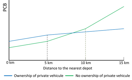
Figure 4.
The cost of the return behaviour according to the distance of the nearest depot.
Since the population density distribution in the areas where people have been surveyed in is unknown, a uniform distribution was assumed for the development of this part of the model. This means that the simulated population’s density is the same throughout a circle with a 15 km radius.
4. Results
This section presents the calibration and validation of the simulation model with data from various Canadian and Quebec sources. A series of experiments was also conducted to observe how the model reacts under different combinations of parameters that are not the base calibration parameters and potentially give insights on the effectiveness of the studied strategy. AnyLogic 7 university edition was used to develop the simulation model and execute the simulation experiments.
4.1. Model Calibration
In the first of two calibration phases, the membership function shapes of the environmental concern segments were adjusted to fit the segmentations in the survey about Quebecers behaviors and attitudes towards the 3R hierarchy (N = 2068) [50]. To validate this aspect, the first values of the matrix were defined: SOV11, SOV22 and SOV33 were set to 100 while the other values were set to 0. The simulation results with this simple diagonal matrix provided a good enough qualitative fit with the estimated percentages of wine bottles found in the province’s curbside collection (blue bin) program [51]. The rest of the matrix was then calibrated using AnyLogic calibration experiment functions.
The original scenario, without the deposit-return scheme, was first quantitatively validated and provided a tight fit within 0.5% of the 85.1% target for the curbside collection value [51]. The values used for γ (µ, σ) in this phase were respectively 1 and 0.
Next, the number of agents needed to be optimized. Figure 5 shows the model stability and validity as a function of the number of replications. Shortly after 10 repetitions, the simulations with 10,000 agents begin to show stable results. However, the simulations with only 2000 agents seems to be the closest to the target value but are less stable.
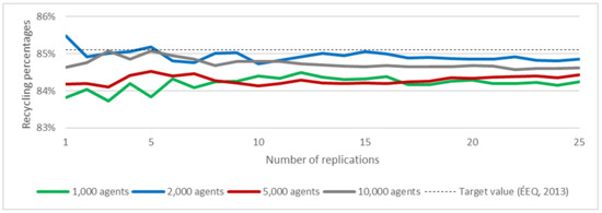
Figure 5.
Curbside collection (blue bin) percentages cumulative averages per number of simulation replications (52 weeks/simulation).
The second phase consisted of the calibration and qualitative validation of the effects of incentives and PBC on the return behavior, as well as the recalibration of the matrix values. Since all these aspects can affect the decision process quite substantially on their own, the calibration had to be done with all of phase 2 parameters at the same time. Thus, to validate the fit of the model, a custom theoretical dataset was calculated to reflect the combination of effects from all the aspects and their respective empirical data. In other words, for every distance bracket, there were two target values, one for agents with cars, and another for agents without. These target values represented the theoretical number of agents that should bring back their bottles according to the incentive value and the effect of the distance to the nearest depot over agents’ return intentions [48]. To reflect the statistical data from Alberta [52,53] and the survey from [54], the incentive values were increased twice over an 8-year period during the simulations in the calibration process to capture the impact of deposit-value increase, in order to be coherent with the empirical data found in the literature. The values used for incentives were adjusted to fit Quebec’s proposed deposit values [48]. Following the 0.05$ increase of the deposit value of wine bottles in Alberta, return rates increased by 4% after 4 years and 6% after 8 years. Data from Alberta was used because it is the only Canadian province to have increased the deposit-values over the past years, thus limiting the model’s validity. As for the CREATE survey [54], it was found that by having a 0.35$ deposit fee on wine bottles, 90% of Quebecers would bring their bottles back to depot centers. In the CROP survey [48], 88.1% of respondents owned a vehicle, which is the percentage used throughout all the simulations performed for the calibration process.
The model was also calibrated to reflect the wine drinking habits of Quebecers with data from the Socitété des Alcools du Québec and Éduc-Alcool. According to the 2016 report of the Société des Alcools du Québec, each Quebecers drank approximately 30.3 bottles of wine in 2016 [55]. However, it would be unreasonable to assume that everyone drinks the same amount of wine through a year. Therefore, data from the 2017 Éduc-Alcool survey on alcohol consumption was used to calibrate a weekly wine consumption distribution [56]. At the end of 25 simulations with 10,000 agents, the average total number of bottles consumed over a year differed from the target value by only +7%.
4.2. Model Validation
Simulations were performed to estimate the product flows resulting from 6 different scenarios. The Figure 6 and Figure 7 display the average percentages of bottles flowing into each EOL options for 10 simulations of each scenario with 52 weeks simulated per simulations. Two groups of scenarios were executed to compare the results with empirical data; the first with a deposit value of 0.15$ and the second with 0.35$. Each scenario group was divided into 3 unique scenarios, which tested three cases of maximum distance between agent to the nearest depot: 5 km, 10 km or 15 km.
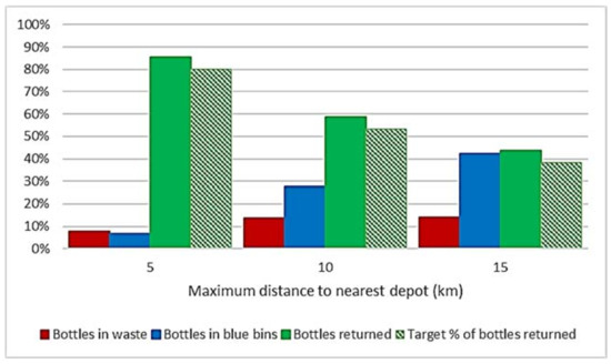
Figure 6.
Averages of 10 simulations for each scenario with a deposit value of 0.15$.
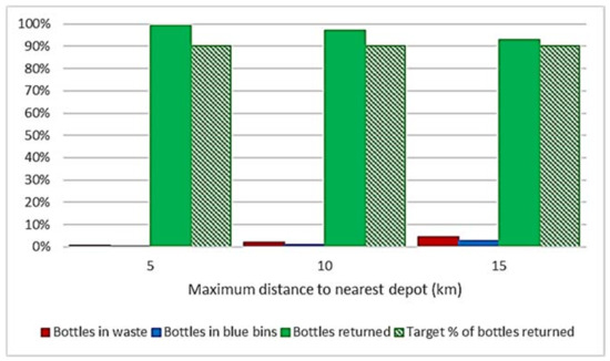
Figure 7.
Averages of 10 simulations for each scenario with a deposit value of 0.35$.
Compared to the empirical data there is an average difference of +5% and +9%, respectively for the 0.15$ [48] and 0.35$ [54] deposit fee scenarios, with the percentages of consumers bringing back their bottles to depot centers in the simulations and in the surveys. However, it must be noted that the empirical data for the 0.35$ deposit value was from a survey that did not specify any distance that would need to be traveled to reach the depot center. Therefore, the target value was the same for each scenario. Nevertheless, the logic that the distance affects the intention to bring back can be seen in both experiences, which greatly contributes to the difference between the simulation results of the 0.35$ deposit value and the empirical data.
To be able to validate this calibrated simulation model quantitatively would require independent survey or a study of an actual deposit-return program in Quebec. Nonetheless, the current model can easily be adapted and calibrated to scenarios and even other products to give some interesting insights to decision-makers and policy-makers.
4.3. Experiments
A series of experiences were conducted with the validated model to obtain insights into how several of the parameters can have an impact on the results. Overall, 18 different scenarios were selected to be analysed with 10 simulation runs of each scenario for a total of 180 simulation runs. As can be seen in Table 1, the scenarios are divided into two group that are each divided again into subgroups. There is no difference between the two main groups beside the deposit value which is, respectively, 0.15$ for the first and 0.35$ for the second. The subgroups represent three different population types characterised by population density and private car ownership. Three different alternatives were tested for each subgroup: 1 depot center, 2 depot centers and 3 depot centers. Populations sizes and densities were inspired from real Quebec cities [57], while the car ownership percentages were estimated with data from Canada, Sweden, United Kingdom and Ireland [58,59,60].

Table 1.
Parameters of the scenarios simulated.
To reflect the regions that these scenarios are based upon, the simulated population size was increased from 10,000 to 50,000. This number of agents was used for all scenarios. In each simulation run, agents and depot centers were randomly placed in a square territory. The sizes of these areas are, respectively, 14.29 km2 for population (A); 50 km2 for (B) and 250 km2 for (C). At the beginning of the simulations, agents select their preferred depot center by calculating the distance between their position and all the depot centers’ positions. They choose the closest one and then always return their bottles to it. Even if an agent never returns a bottle, they will still have a preferred depot center. Also, if two depot centers are equally distanced from a consumer agent’s position, the agent will randomly choose one or the other when the simulation begins.
In the following sections, only the results of the first group will be presented because there is no significant difference between all the results of the second group. Each of the nine scenarios produced average return percentages above 95% with very low standard deviations.
Graphical representations of the scenarios can be seen in Appendix A, where the agents are presented with colored humanoid shapes (black for non-drinkers, red for those who put their bottles to waste, yellow for those who put their bottles in the curbside collection program and green for those who return their bottles to depot centers). The color of these agents is defined by their last behavior. Depot centers are presented as blue buildings.
4.3.1. Model Stability
In a similar way to how the model was calibrated, model stability had to be verified since the scenarios are different than the base scenario used for calibration. Figure 8 illustrates the results of the model stability under the new scenarios. It appears that the cumulative averages for each scenario, both for the percentage of returned bottles and the number of bottles returned per depot center, tend to stabilize after 4 simulations. These results indicate that, even by adding multiple depot centers, increasing the population size and varying the percentages of private car ownership outside the base calibration scenario values, the model remains stable.
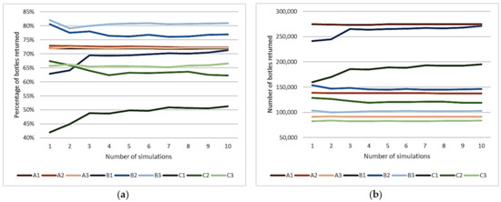
Figure 8.
(a) The cumulative average percentage of bottles returned for 10 successive simulations runs; (b) the cumulative average of the number of bottles returned, with all depot centers combined, for 10 successive simulations runs.
4.3.2. Bottle Returns Percentages
The Table 2 below shows the percentages of bottles returned by the populations. The results indicate that the number of bottles returned is proportional to the number of depot centers. The only exception is scenario A2 (population A with 2 depot centers), where the average and maximum return percentages are slightly higher than scenario A3. Given that these results are extremely close, a higher number of repetitions could most certainly bring the return percentages of scenario A3 above those of scenario A2.
Table 2.
The percentages of bottles returned for 10 simulations of each scenario.
Another observation is that, the suburban population type seems to be the most efficient at returning bottles. Considering that suburban population territory is nearly 3 times the size of the urban population territory, the percentage of car ownership appears to have a greater positive effect on the return percentages than the negative effect of the distance between the nearest depot center. However, the lower return percentages of the rural population also indicate that there is a threshold where the dissuading effect of the distance becomes greater than advantages of easily accessible transportation, even if the number of consumers owning a private vehicle increases.
For the urban population, there is no clear indication on which scenario would be better on a logistical standpoint alone. For such cases, economic considerations on the costs of depot centers operations would be mandatory to identify the optimal scenario. For the suburban population, the maximum of scenario B1 is respectively only around 1% and 2.5% below the average and maximum of scenario B3. These findings show that even if the suburban population return their bottles the most, positioning of the depot centers can considerably alter the efficiency of the strategy. For the rural population, the results support the findings of the (B) population.
4.3.3. Number of Bottles Returned in Depot Center
The Table 3 and Table 4 shows the averages and the number of bottles returned per depot centers. Illustrations of the results can be found in Appendix B and Appendix C.
Table 3.
Average number of bottles returned per depot centers for 10 simulations of each scenario.
Table 4.
Number of bottles returned per depot centers for 10 simulations of each scenario.
Consistent with the previous results, all the maximum average values from the urban populations are lower that the maximum averages of the suburban population. Interestingly, the maximum average of scenario C3 is only 695 bottles behind the maximum average of the A3 population. Therefore, even across 250 km2, if the depots are optimally positioned, the bottle return potential is similar to the urban population, which fits in less than 15 km2. However, the higher standard deviation and the lower average values for the rural scenarios indicates that the effectiveness of the strategy is crucially dependent of the depot centers’ placements. The similar standard deviations values of scenarios B1 and C1 also suggests that even if the distance increases considerably, a slight increase in the percentage of private vehicle ownership is enough to stabilize the results around the mean.
As for the number of bottles per depot centers, the averages for the urban and suburban scenarios are considerably similar. On the other hand, the standard deviations of the (A) population are all much lower than the (B), which indicates that the first population is less sensitive to the depot center locations than its counterparts. Nevertheless, with only one depot center strategically placed, it is possible in the suburban population to surpass the maximum number of bottles returned for population (A), even if its average is lower.
It must be noted that increasing the number of depot centers can have some unexpected effects. For populations (A) and (B), there is a steep augmentation in the standard deviations between 1 and 2 depot centers. It then seems to lower as the number of depot center keeps increasing. The model can cause this phenomenon itself, since agents have a preferred depot center. In reality, the split between the amount of bottle returned would probably be less intense since agents could potentially go to both depot centers depending on their travel habits. It is still reasonable to assume that beyond two depot centers the standard deviation decreases continually, after having a peak between one and two depot centers.
5. Discussion
The proposed simulation model, along with the calibration process and series of experiences, enables the analysis a potential EOL product flow strategy that is, at the time of the study, still at a proposition phase. Waste management and EOL product flow strategies usually have large scale implications and impacts. If these strategies are not thoroughly analysed before they are developed, they can have unexpected negative impacts or simply be ineffective and become a waste of time and resources [5]. The two following section presents the general insights provided by the model as well as its limitations.
5.1. General Insights
The results shown in Table 2, Table 3 and Table 4 give insights into the relative importance of several parameters of the model over the return percentage behavior. While the results are not to be taken as quantitively accurate evidence, they most certainly provide some qualitative evidence. First, there is no doubt that the value of the deposit has a significant impact on the decision of the consumers. Coherent with the empirical data [54], a deposit value of 0.35$ provides some striking results with a 95% minimum return rate, regardless of the population. These results are in line with Canadian data, where the deposit fee in Ontario for wine and spirits bottles is respectively 0.10$ and 0.20$ for bottles below and above 630 mL. The Ontario recycling rate is 87%, which is not the percentage of bottles returned, but rather the percentage of bottles that were returned and recycled [53]. Results also suggests that the distance to the nearest depot and the ownership of private vehicle can have a substantial impact on return percentages. Between the two, the second seems to have a greater impact than the distance, up to a certain point. It is, however, difficult to identify where this threshold stands with this paper’s experiments. Another finding is that the positioning of the depot centers would be crucial to the success of the strategy. For example, when there is only one depot center, the urban population returns more bottles on average, but a well-positioned depot center in the suburban population can result in a higher return percentage. For this specific case, the maximum return percentage of the suburban population for one depot center is 9.5% above the maximum of the urban population for its equivalent scenario.
The simulation model can also be used to give insights into the capacity needed for the depot centers. Since the model was calibrated with Quebecers’ wine consumption, it is possible to even estimate the costs of specific scenarios with their respective depot centers capacity needs. Data on the estimation of depot centers operations costs can be found in a report produced for the Société des Alcools du Québec [61].
5.2. Model Limitations and Future Works
The simulation model proposed in this paper is not to be taken without its limitations. Future works will focus on using heterogeneous populations. At the moment, results are altered by the fact that the populations (A), (B) and (C) used in the experiments are homogeneous. Real-life cities and districts are not homogeneous. Therefore, replication of this paper’s experiments with heterogeneous populations may produce substantially different results.
Another limitation of the model is that it was calibrated with a 0 to 15 km territory. Thus, the calculation of the PBC beyond 15 km, especially for the rural scenarios, may not be accurate. Nevertheless, having simulated territories defined as closed squares also adds some level of inconsistency. For example, in scenario C1, agents that are located near the borders of the territory and far from the depot centers could actually be near another depot center from an adjacent territory. Hence, the 15 km calibration limit may not be as much of an impacting factor as the simulated territories size limitations.
Considering that the survey used for the calibration of the PBC had 88.1% of the participants owning a vehicle at the time of the study [48], compared to the empirical data used to define the experiences [58,59,60], the percentage of private vehicle ownership may have been overestimated in the calibration process. While the main reason to own a vehicle is to facilitate travel over longer distances, participants from the survey could be more sensible to travel distances. Consequently, the impact of the distance to the nearest depot on the populations analyzed in the experiments may not be accurately representative of how comparable real populations would behave over this aspect.
One last notable limitation of the model is how agents have preferred depot centers. Future works will enable agents to have multiple favorite depot centers. For instance, within a 10% distance range, agents could alternate between multiple accessible depot centers.
6. Conclusions
Even with its limitations, this model could be used by policymakers to obtain insights into various aspects of the studied strategy, such as the deposit value as well as the size and placement of depot centers. However, the simulation model must not be taken as an optimisation tool. The model could compare specific scenarios of depot center sizes and placements for example, but they must be defined beforehand. The accuracy of the model must also be taken in to account, as, for the time being, it can only represent homogeneous populations. Thus, it is more suitable for small- to medium-scale cities. Indeed, extensive work needs to be done before the model can simulate large scale cities that have significant variations in their population density.
The proposed model builds upon the existing literature by taking an approach that enables the simulation of multiple and complex behaviors. The model also integrates parts of the logistics aspect that recycling behavior simulations do not usually consider.
The implementation of agent-based modeling and simulation into municipal waste management system strategies analysis enables the reproduction of complex behaviors that are crucial when studying systems that are human-driven. Using artificial societies to empower the circular economy ideology seems more than appropriate when considering that this framework addresses large-scale networks that are composed of many entities with their own behaviors and characteristics that can be represented by autonomous agents. This paper proposes a methodology to apply behavior models with the help of appropriate empirical data to analyse mass flow driven by human decisions and complex social interactions. Future research will focus on adding socio-demographic characteristics to the populations, in order to take into account their heterogeneity, as well as the impact of social networks and media on consumer behavior. The model will then be used to simulate scenarios with populations that are based on actual cities and evaluate their respective performances. Eventually, the model could also be adapted to new products and analyse other waste diversion strategies such as centralized depot centers that accept multiple EOL products. Even if some aspect of the model were less successfully captured, the first attempt at calibrating and validating the model has proven to be substantially successful and opens the doors to multi-disciplinary models where psychology, computer simulation and engineering experts can thrive on common objectives.
Future research will also use the developed methodology and model to estimate the environmental impacts and costs of alternative municipal waste management strategies within a CE framework. Jointly with the construction costs and operating costs of depot centers according to their sizes and capacities [61], multiple logistic strategies can be analysed and compared. By enabling decision-makers and policy-makers to gain insights into the efficiencies of potential end-of-life product flow strategies, the risk associated with implementing large-scale strategies can be greatly diminished. To further increase the potential success of these strategies, pilot projects can be used to re-calibrate and re-validate existing consumer behavior models with new data to find the optimal solutions for specific populations and regions.
Author Contributions
Conceptualization, A.L. and J.-M.F.; Data curation, A.L.; Formal analysis, A.L.; Funding acquisition, J.-M.F.; Investigation, A.L.; Methodology, A.L. and J.-M.F.; Project administration, A.L. and J.-M.F.; Resources, A.L. and J.-M.F.; Software, A.L.; Supervision, J.-M.F.; Validation, A.L. and J.-M.F.; Visualization, A.L.; Writing—original draft, A.L.; Writing—review and editing, J.-M.F.
Funding
This research received no external funding.
Conflicts of Interest
The authors declare no conflict of interest.
Appendix A. Graphical Representations of the Scenarios Produced with AnyLogic

Figure A1.
Presents one of the 10 simulations executed for each scenario with a 0.15$ deposit value. (a) Scenario A1; (b) Scenario A2; (c) Scenario A3; (d) Scenario B1; (e) Scenario B2; (f) Scenario B3; (g) Scenario C1; (h) Scenario C2; (i) Scenario C3.
Figure A1.
Presents one of the 10 simulations executed for each scenario with a 0.15$ deposit value. (a) Scenario A1; (b) Scenario A2; (c) Scenario A3; (d) Scenario B1; (e) Scenario B2; (f) Scenario B3; (g) Scenario C1; (h) Scenario C2; (i) Scenario C3.


Figure A2.
Presents one of the 10 simulations executed for each scenario with a 0.35$ deposit value. (a) Scenario A1; (b) Scenario A2; (c) Scenario A3; (d) Scenario B1; (e) Scenario B2; (f) Scenario B3; (g) Scenario C1; (h) Scenario C2; (i) Scenario C3.
Figure A2.
Presents one of the 10 simulations executed for each scenario with a 0.35$ deposit value. (a) Scenario A1; (b) Scenario A2; (c) Scenario A3; (d) Scenario B1; (e) Scenario B2; (f) Scenario B3; (g) Scenario C1; (h) Scenario C2; (i) Scenario C3.


Appendix B. Average Number of Bottles Returned Per Depot Center for Each Simulation Run

Figure A3.
Average number of bottles returned per depot center for the simulations of the three scenarios A with a 0.15$ deposit value.
Figure A3.
Average number of bottles returned per depot center for the simulations of the three scenarios A with a 0.15$ deposit value.


Figure A4.
Average number of bottles returned per depot center for the simulations of the three scenarios B with a 0.15$ deposit value.
Figure A4.
Average number of bottles returned per depot center for the simulations of the three scenarios B with a 0.15$ deposit value.


Figure A5.
Average number of bottles returned per depot center for the simulations of the three scenarios C with a 0.15$ deposit value.
Figure A5.
Average number of bottles returned per depot center for the simulations of the three scenarios C with a 0.15$ deposit value.

Appendix C. Number of Bottles Returned Per Depot Center for Each Simulation Run

Figure A6.
Number of bottles returned per depot center for the simulations of the three scenarios A with a 0.15$ deposit value.
Figure A6.
Number of bottles returned per depot center for the simulations of the three scenarios A with a 0.15$ deposit value.


Figure A7.
Number of bottles returned per depot center for the simulations of the three scenarios A with a 0.15$ deposit value.
Figure A7.
Number of bottles returned per depot center for the simulations of the three scenarios A with a 0.15$ deposit value.


Figure A8.
Number of bottles returned per depot center for the simulations of the three scenarios A with a 0.15$ deposit value.
Figure A8.
Number of bottles returned per depot center for the simulations of the three scenarios A with a 0.15$ deposit value.

References
- Zaman, A.U. A comprehensive study of the environmental and economic benefits of resource recovery from global waste management systems. J. Clean. Prod. 2016, 124, 41–50. [Google Scholar] [CrossRef]
- Karmperis, A.C.; Aravossis, K.; Tatsiopoulos, I.P.; Sotirchos, A. Decision support models for solid waste management: Review and game-theoretic approaches. Waste Manag. 2013, 33, 1290–1301. [Google Scholar] [CrossRef] [PubMed]
- Soltani, A.; Hewage, K.; Reza, B.; Sadiq, R. Multiple stakeholders in multi-criteria decision-making in the context of municipal solid waste management: A review. Waste Manag. 2015, 35, 318–328. [Google Scholar] [CrossRef] [PubMed]
- Borshchev, A. The Big Book of Simulation Modeling: Multimethod Modeling with AnyLogic 6; AnyLogic North America: Chicago, IL, USA, 2013. [Google Scholar]
- Goddard, H.C. The benefits and costs of alternative solid waste management policies. Resour. Conserv. Recycl. 1995, 13, 183–213. [Google Scholar] [CrossRef]
- Bohm, R.A.; Folz, D.H.; Kinnaman, T.C.; Podolsky, M.J. The costs of municipal waste and recycling programs. Resour. Conserv. Recycl. 2010, 54, 864–871. [Google Scholar] [CrossRef]
- Lakhan, C. Diversion, but at what cost? The economic challenges of recycling in Ontario. Resour. Conserv. Recycl. 2015, 95, 133–142. [Google Scholar] [CrossRef]
- Cleary, J. Life cycle assessments of municipal solid waste management systems: A comparative analysis of selected peer-reviewed literature. Environ. Int. 2009, 35, 1256–1266. [Google Scholar] [CrossRef] [PubMed]
- De Feo, G.; Malvano, C. The use of LCA in selecting the best MSW management system. Waste Manag. 2009, 29, 1901–1915. [Google Scholar] [CrossRef] [PubMed]
- Fitzgerald, G.C.; Krones, J.S.; Themelis, N.J. Greenhouse gas impact of dual stream and single stream collection and separation of recyclables. Resour. Conserv. Recycl. 2012, 69, 50–56. [Google Scholar] [CrossRef]
- Simon, B.; Amor, M.B.; Földényi, R. Life cycle impact assessment of beverage packaging systems: Focus on the collection of post-consumer bottles. J. Clean. Prod. 2016, 112, 238–248. [Google Scholar] [CrossRef]
- Komly, C.E.; Azzaro-Pantel, C.; Hubert, A.; Pibouleau, L.; Archambault, V. Multiobjective waste management optimization strategy coupling life cycle assessment and genetic algorithms: Application to PET bottles. Resour. Conserv. Recycl. 2012, 69, 66–81. [Google Scholar] [CrossRef]
- Vellini, M.; Savioli, M. Energy and environmental analysis of glass container production and recycling. Energy 2009, 34, 2137–2143. [Google Scholar] [CrossRef]
- Ghinea, C.; Drăgoi, E.N.; Comăniţă, E.D.; Gavrilescu, M.; Câmpean, T.; Curteanu, S.; Gavrilescu, M. Forecasting municipal solid waste generation using prognostic tools and regression analysis. J. Environ. Manag. 2016, 182, 80–93. [Google Scholar] [CrossRef] [PubMed]
- Thøgersen, J. Recycling and morality: A critical review of the literature. Environ. Behav. 1996, 28, 536–558. [Google Scholar] [CrossRef]
- Stern, P.C. New environmental theories: Toward a coherent theory of environmentally significant behavior. J. Soc. Issues 2000, 56, 407–424. [Google Scholar] [CrossRef]
- Sidique, S.F.; Joshi, S.V.; Lupi, F. Factors influencing the rate of recycling: An analysis of Minnesota counties. Resour. Conserv. Recycl. 2010, 54, 242–249. [Google Scholar] [CrossRef]
- Sidique, S.F.; Lupi, F.; Joshi, S.V. The effects of behavior and attitudes on drop-off recycling activities. Resour. Conserv. Recycl. 2010, 54, 163–170. [Google Scholar] [CrossRef]
- López-Mosquera, N.; Lera-López, F.; Sánchez, M. Key factors to explain recycling, car use and environmentally responsible purchase behaviors: A comparative perspective. Resour. Conserv. Recycl. 2015, 99, 29–39. [Google Scholar] [CrossRef]
- Babaei, A.A.; Alavi, N.; Goudarzi, G.; Teymouri, P.; Ahmadi, K.; Rafiee, M. Household recycling knowledge, attitudes and practices towards solid waste management. Resour. Conserv. Recycl. 2015, 102, 94–100. [Google Scholar] [CrossRef]
- Bissing-Olson, M.J.; Fielding, K.S.; Iyer, A. Experiences of pride, not guilt, predict pro-environmental behavior when pro-environmental descriptive norms are more positive. J. Environ. Psychol. 2016, 45, 145–153. [Google Scholar] [CrossRef]
- Tucker, P. Normative influences in household waste recycling. J. Environ. Plan. Manag. 1999, 42, 63. [Google Scholar] [CrossRef]
- Steg, L.; Vlek, C. Encouraging pro-environmental behaviour: An integrative review and research agenda. J. Environ. Psychol. 2009, 29, 309–317. [Google Scholar] [CrossRef]
- Best, H.; Mayerl, J. Values, beliefs, attitudes: An empirical study on the structure of environmental concern and recycling participation. Soc. Sci. Q. 2013, 94, 691–714. [Google Scholar] [CrossRef]
- Gifford, R.; Nilsson, A. Personal and social factors that influence pro-environmental concern and behaviour: A review. Int. J. Psychol. 2014, 49, 141–157. [Google Scholar] [CrossRef] [PubMed]
- Kormos, C.; Gifford, R. The validity of self-report measures of proenvironmental behavior: A meta-analytic review. J. Environ. Psychol. 2014, 40, 359–371. [Google Scholar] [CrossRef]
- Morren, M.; Grinstein, A. Explaining environmental behavior across borders: A meta-analysis. J. Environ. Psychol. 2016, 47, 91–106. [Google Scholar] [CrossRef]
- Ajzen, I. The theory of planned behavior. Organ. Behav. Hum. Decis. Process. 1991, 50, 179–211. [Google Scholar] [CrossRef]
- Tonglet, M.; Phillips, P.S.; Read, A.D. Using the Theory of Planned Behaviour to investigate the determinants of recycling behaviour: A case study from Brixworth, UK. Resour. Conserv. Recycl. 2004, 41, 191–214. [Google Scholar] [CrossRef]
- White, K.M.; Hyde, M.K. The role of self-perceptions in the prediction of household recycling behavior in Australia. Environ. Behav. 2012, 44, 785–799. [Google Scholar] [CrossRef]
- Chan, L.; Bishop, B. A moral basis for recycling: Extending the theory of planned behaviour. J. Environ. Psychol. 2013, 36, 96–102. [Google Scholar] [CrossRef]
- Rhodes, R.E.; Beauchamp, M.R.; Conner, M.; Bruijn, G.J.D.; Kaushal, N.; Latimer-Cheung, A. Prediction of depot-based specialty recycling behavior using an extended theory of planned behavior. Environ. Behav. 2015, 47, 2. [Google Scholar] [CrossRef]
- Botetzagias, I.; Dima, A.-F.; Malesios, C. Extending the theory of planned behavior in the context of recycling: The role of moral norms and of demographic predictors. Resour. Conserv. Recycl. 2015, 95, 58–67. [Google Scholar] [CrossRef]
- Tucker, P.; Murney, G.; Lamont, J. Predicting recycling scheme performance: A process simulation approach. J. Environ. Manag. 1998, 53, 31–48. [Google Scholar] [CrossRef]
- Tucker, P.; Smith, D. Simulating household waste management behaviour. J. Artif. Soc. Soc. Simul. 1999, 2, 31. [Google Scholar]
- Bonabeau, E. Agent-based modeling: Methods and techniques for simulating human systems. Proc. Natl. Acad. Sci. USA 2002, 99 (Suppl. 3), 7280–7287. [Google Scholar] [CrossRef] [PubMed]
- Kiesling, E.; Günther, M.; Stummer, C.; Wakolbinger, L.M. Agent-based simulation of innovation diffusion: A review. Cent. Eur. J. Oper. Res. 2012, 20, 183–230. [Google Scholar] [CrossRef]
- Scalco, A.; Ceschi, A.; Shiboub, I.; Sartori, R.; Frayret, J.M.; Dickert, S. The implementation of the theory of planned behavior in an agent-based model for waste recycling: A review and a proposal. In Agent-Based Modeling of Sustainable Behaviors; Springer: Berlin/Heidelberg, Germany, 2017; pp. 77–97. [Google Scholar]
- Schwarz, N.; Ernst, A. Agent-based modeling of the diffusion of environmental innovations—An empirical approach. Technol. Forecast. Soc. Chang. 2009, 76, 497–511. [Google Scholar] [CrossRef]
- Kaufmann, P.; Stagl, S.; Franks, D.W. Simulating the diffusion of organic farming practices in two New EU Member States. Ecol. Econ. 2009, 68, 2580–2593. [Google Scholar] [CrossRef]
- Ceschi, A.; Dorofeeva, K.; Sartori, R.; Dickert, S.; Scalco, A. A Simulation of Householders’ Recycling Attitudes Based on the Theory of Planned Behavior. In Trends in Practical Applications of Agents, Multi-Agent Systems and Sustainability; Springer: Berlin/Heidelberg, Germany, 2015; pp. 177–184. [Google Scholar]
- Ghali, M.R.; Frayret, J.-M.; Ahabchane, C. Agent-Based Model of Self-Organized Industrial Symbiosis. J. Clean. Prod. 2017, 161, 452–465. [Google Scholar] [CrossRef]
- Shi, X.; Thanos, A.E.; Celik, N. Multi-objective agent-based modeling of single-stream recycling programs. Resour. Conserv. Recycl. 2014, 92, 190–205. [Google Scholar] [CrossRef]
- Wang, B.; Brême, S.; Moon, Y.B. Hybrid modeling and simulation for complementing Lifecycle Assessment. Comput. Ind. Eng. 2014, 69, 77–88. [Google Scholar] [CrossRef]
- Armitage, C.J.; Conner, M. Efficacy of the theory of planned behaviour: A meta-analytic review. Br. J. Soc. Psychol. 2001, 40, 471–499. [Google Scholar] [CrossRef] [PubMed]
- Rai, V.; Robinson, S.A. Agent-based modeling of energy technology adoption: Empirical integration of social, behavioral, economic, and environmental factors. Environ. Model. Softw. 2015, 70, 163–177. [Google Scholar] [CrossRef]
- Maki, A.; Burns, R.J.; Long, H.; Rothman, A.J. Paying people to protect the environment: A meta-analysis of financial incentive interventions to promote proenvironmental behaviors. J. Environ. Psychol. 2016, 47, 242–255. [Google Scholar] [CrossRef]
- CROP. Comportements des Québécois Dans L'éventualité d'un Élargissement de la Consigne; CROP: Montreal, QC, Canada, 2015. [Google Scholar]
- Sidique, S.F.; Lupi, F.; Joshi, S.V. Estimating the demand for drop-off recycling sites: A random utility travel cost approach. J. Environ. Manag. 2013, 127, 339–346. [Google Scholar] [CrossRef] [PubMed]
- SOM. Portrait des Comportements et Attitudes des Citoyens Québécois à L’égard des 3RV; SOM: Montreal, QC, Canada, 2015. [Google Scholar]
- Éco-Entreprise Québec (ÉEQ). Caractérisation des Matières Résiduelles du Secteur Résidentiel au Québec 2012–2013; Éco-Entreprise Québec: Montreal, QC, Canada, 2013. [Google Scholar]
- CM Consulting. Who Pays What: An Analysis of Beverage Container Collection and Costs in Canada; CM Consulting: Barcelona, Spain, 2014. [Google Scholar]
- CM Consulting. Who Pays What: An Analysis of Beverage Container Collection and Costs in Canada; CM Consulting: Barcelona, Spain, 2016. [Google Scholar]
- CREATE. Étude Comparative des Systèmes de Récupération des Contenants de Boisson au Québec; CREATE: Montreal, QC, Canada, 2015. [Google Scholar]
- SAQ. Rapport Annuel 2016; SAQ: Montreal, QC, Canada, 2016. [Google Scholar]
- Éduc-Alcool. Les Québécois et L'alcool 2017; Éduc-Alcool: Montreal, QC, Canada, 2017. [Google Scholar]
- Institut de la statistique du Québec. Recensement et Enquête Nationale Auprès des Ménages de 2011; Statistique Canada: Ottawa, ON, Canada, 2011. [Google Scholar]
- Turcotte, M. % of Population Aged 18 and over Making All Trips by Car (as a Driver or Passenger) on the Reference Day, by Census Metropolitan Area (CMA); Statistique Canada: Ottawa, ON, Canada, 2008.
- Roque, D.; Masoumi, H.E. An analysis of car ownership in Latin American cities: A perspective for future research. Periodica Polytechnica. Transp. Eng. 2016, 44, 5. [Google Scholar]
- Pyddoke, R.; Creutzer, C. Household Car Ownership in Urban and Rural Areas in Sweden 1999–2008; Centre for Transport Studies: Stockholm, Sweden, 2014. [Google Scholar]
- LIDD. Présentation du Rapport Final (Sommaire Exécutif); LIDD: Montreal, QC, Canada, 2015. [Google Scholar]


© 2018 by the authors. Licensee MDPI, Basel, Switzerland. This article is an open access article distributed under the terms and conditions of the Creative Commons Attribution (CC BY) license (http://creativecommons.org/licenses/by/4.0/).