An Automated Capacity-Allocating-Based Transition Strategy Between Harmonic and Reactive Power Compensation for Multifunctional PAPF

Abstract

This paper proposes a practical heuristic engineering strategy for automated capacity allocation in a multifunctional parallel active power filter (PAPF) that simultaneously provides harmonic and reactive power compensation. Unlike theoretically optimal methods, our approach prioritizes real-time feasibility and ease of implementation. The key features are: (1) an event-triggered, closed-loop THD-feedback mechanism that dynamically recalculates the minimum active power required for harmonic compensation only when the load harmonic content changes, avoiding periodic computational waste; (2) a strict priority handling that guarantees grid current THD below 5% (IEEE-519 compliant) under all operating conditions, even when capacity is severely insufficient; (3) a closed-loop transition mechanism that uses measured grid current THD and remaining capacity as feedback inputs to continuously adapt power distribution. The proposed rule-based strategy does not claim theoretical optimality but provides a verifiable, ready-to-implement solution with experimental evidence. Simulation and experimental results on a three-level NPC PAPF prototype demonstrate that the strategy maintains grid current THD below 5% while keeping the apparent power within the rated capacity, achieving near-optimal reactive compensation (92–96% of the optimum) without iterative optimization. The experimental validation includes efficiency measurements, switching-loss estimation, DSP timing analysis, and robustness tests under grid disturbances. Future work will extend the concept to multi-inverter systems using multi-objective optimization and AI-based allocation.

1. Introduction

In recent years, power distribution systems have faced increasingly severe power quality challenges, primarily manifested as frequency fluctuations, voltage distortion, and current harmonics [1,2,3]. With the widespread adoption of nonlinear loads, harmonic pollution has emerged as a critical threat to the stable operation of power systems [4]. As a conventional solution, passive power filters (PPFs) have gained extensive application in harmonic suppression due to their cost-effectiveness, simple topology, and high operational efficiency [5]. However, inherent limitations of PPFs, including sluggish dynamic response, susceptibility to system resonance, and sensitivity to grid parameters [6,7], have driven researchers to explore superior alternatives.

In this context, active power filters (APFs) have emerged as next-generation harmonic mitigation devices. Studies demonstrate that APFs not only effectively overcome the technical bottlenecks of PPFs but also exhibit enhanced harmonic compensation capabilities, offering innovative solutions for future power quality management [8,9]. Significant progress has been made in optimizing APF harmonic compensation algorithms. For example, a vector resonant controller to address harmonic oscillation suppression was introduced in [10]. The study in [11] developed a comb filter strategy based on an improved second-order generalized integrator, achieving superior harmonic suppression accuracy. A selective harmonic-controlled PWM modulator was designed in [12], which involved integrated artificial neural networks with sequential quadratic programming. In [13], a quasi-proportional resonant control algorithm with phase-lead characteristics was proposed, enabling closed-loop integration of harmonic detection and control. Nevertheless, existing APF systems are predominantly designed for light-load conditions, resulting in underutilized redundant capacity and suboptimal operational efficiency.

Notably, modern distribution networks exhibit increasingly complex load characteristics, where harmonic pollution coexists with substantial reactive power demand [14]. This dual challenge exacerbates operational risks for grid equipment, rendering traditional single-function compensation devices inadequate. Given the high costs associated with deploying dedicated compensation equipment, leveraging the redundant capacity of APFs for multifunctional power quality regulation has become a research focus [15,16]. By optimizing inverter control strategies to enable APFs to provide reactive power compensation alongside harmonic mitigation, this approach not only enhances device utilization but also reduces system retrofitting costs.

Preliminary achievements have been made in APF multifunctional applications. Reference [17] established a harmonic evaluation framework based on IEEE Standard 1459 and implemented coordinated harmonic and reactive compensation via space vector PWM. An equivalent conductance method for compensation reference calculation was proposed in [18], improving hybrid compensation accuracy. However, these studies inadequately address APF power constraints, while optimal power allocation during compensation is crucial for ensuring system safety and economic efficiency. Particularly under APF capacity limitations, dynamic power allocation between harmonic suppression and reactive compensation remains a critical unresolved issue.

Furthermore, conventional APF control strategies predominantly adopt global compensation modes [19,20,21,22], which deliver desired performance under sufficient capacity conditions. However, this “one-size-fits-all” approach leads to significant performance degradation when device capacity is constrained [23]. Therefore, developing an adaptive power allocation mechanism under capacity constraints to dynamically coordinate harmonic and reactive compensation is essential for enhancing APF effectiveness. Although a capacity-limited current control method for APFs was proposed in [24], it focused solely on active current components while neglecting harmonic compensation efficacy.

To overcome these challenges, this paper proposes an advanced control strategy for a multifunctional parallel active power filter (PAPF) that enables simultaneous harmonic and reactive power compensation. The primary novelty of this paper consists of three distinguishable aspects:

(1)

Real-time THD-feedback-based automated capacity allocation, rather than fixed thresholds: The minimum active power required for harmonic compensation is dynamically recalculated only when the load harmonic content changes (event-triggered), thereby avoiding periodic recalculations that waste computational resources and may cause unnecessary transients.

(2)

A clear priority handling mechanism: Even under severe capacity insufficiency, harmonic compensation is strictly prioritized over reactive power compensation, ensuring that the grid current THD is always maintained below 5%—a guarantee that existing multifunctional APF strategies do not provide.

(3)

A closed-loop transition mechanism: Unlike conventional open-loop or rule-based power allocation, the proposed strategy simultaneously uses the measured grid current THD and the remaining capacity PremainPremain as feedback inputs, forming a closed-loop control that continuously adapts the power distribution between harmonic suppression and reactive power compensation.

With these features, the proposed PAPF system achieves better utilization of available resources compared to conventional systems, maintains the apparent power within the rated capacity, and enables automated transition between compensation modes even under dynamic changes of nonlinear loads.

This paper is organized as follows. Section 2 contains the description of the overall multifunctional PAPF system. Section 3 proposes an automated transition strategy between harmonic and reactive power compensation, including the active power regulation of DC bus-side and the reactive power control of the PAPF inverter. In addition, the harmonic compensation process is presented in detail. Section 4 tests the control strategy of this PAPF system with different nonlinear load conditions. Experimental results on the feasibility of the proposed method are given in Section 5. Finally, Section 6 concludes the whole paper. The symbols and notations used in the text are shown in

Table 1. Nomenclature.

Symbol	Description	Symbol	Description
THDIs	Grid current total harmonic distortion	Pmin	Minimum active power required for harmonic compensation
THDload	Load current total harmonic distortion	Premain	Remaining capacity after allocating Pmin
THDIh	Harmonic component of load current THD	Pinverter	Active power output of PAPF inverter
THDtop	Upper THD limit for harmonic compensation	Pdc	Output active power from DC bus
THDbottom	Lower THD limit for harmonic compensation	PL	Load active power
	PAPF active power	PS	Grid active power
QL	Load reactive power demand	idc	DC-side current
QPC	PAPF reactive power output	iq	q-axis current reference for reactive power control
QMAX	Maximum compensable reactive power without degrading harmonic compensation	Vdc	DC-bus voltage
Srated	Rated capacity of PAPF inverter	OPM	Operating mode

.

2. Power Quantities and Power Quality Analysis

The effective current I_eff is defined in (1) as a function of phase currents and neutral line current, which primarily incorporates RMS values of both the fundamental and harmonic current components. The specific formulation is expressed as follows:

$$\begin{array}{c}{I}_{eff}=\sqrt{{\displaystyle \frac{I_a^2+I_b^2+I_c^2+I_n^2}{3}}}=\sqrt{I_{eff\_f}^2+I_{eff\_h}^2}\end{array}$$

(1)

where I_a, I_b, and I_c are the line currents, respectively. I_{eff_f} and I_{eff_h} are the effective fundamental harmonic current, respectively.

The effective voltage V_eff defined in (2) is a function of the measured point voltages. This definition incorporates the RMS values of the fundamental and harmonic voltage components, as detailed below.

$$\begin{array}{c}{V}_{eff}=\sqrt{{\displaystyle \frac{3\left(V_a^2+V_b^2+V_c^2\right)+\left(V_{ab}^2+V_{bc}^2+V_{ca}^2\right)}{18}}}=\sqrt{V_{eff\_f}^2+V_{eff\_h}^2}\end{array}$$

(2)

where V_a, V_b, V_c are the phase voltages of abc phases, and V_ab, V_bc, V_ca are the line voltages. V_{eff_f} and V_{eff_h} are the fundamental and harmonic component of the effective voltage, respectively. The effective apparent power S_eff is shown below:

$$\begin{array}{c}{S}_{eff}=3V_{eff}{I}_{eff}\end{array}$$

(3)

Replacing the effective voltage and current in (3) with the fundamental and non-fundamental values, the apparent power of fundamental and harmonic power, S_{eff_f} and S_{eff_h}, can be obtained:

$$\begin{array}{c}{S}_{eff\_f}=3V_{eff\_f}{I}_{eff\_f}\end{array}$$

(4)

$$\begin{array}{c}{S}_{eff\_h}=\sqrt{S_{eff}^2-S_{eff\_f}^2}=3\sqrt{{(V_{eff\_f}{I}_{eff\_h})}^2+{(V_{eff\_h}{I}_{eff\_f})}^2+{(V_{eff\_h}{I}_{eff\_h})}^2}\end{array}$$

(5)

In (4), by introducing the fundamental positive sequence of active power P⁺_f, reactive power Q⁺_f and the unbalanced power, S_ub, the effective apparent power of fundamental component S_{eff_f} is expressed as:

$$\begin{array}{c}{S}_{eff\_f}=\sqrt{{\left(P_f^{+}\right)}^2+{\left(Q_f^{+}\right)}^2+{(S_{ub})}^2}\end{array}$$

(6)

In (6), P⁺_f, Q⁺_f and S_ub can be derived by:

$$\begin{array}{c}{P}_f^{+}=3V_f^{+}{I}_f^{+}\cos {\theta }_f^{+}\end{array}$$

(7)

$$\begin{array}{c}{Q}_f^{+}=3V_f^{+}{I}_f^{+}\sin {\theta }_f^{+}\end{array}$$

(8)

$$\begin{array}{c}{S}_{ub}=\sqrt{{(S_{eff\_f})}^2-{\left(P_f^{+}\right)}^2-{\left(Q_f^{+}\right)}^2}\end{array}$$

(9)

where V⁺_f, I⁺_f are the positive sequence voltage and current, respectively. θ⁺_f is the phase shift angle between V⁺_f and I⁺_f. In addition, all the voltages and currents in (7) and (8) are effective values.

The power factor PF_eff in (10) is defined as the active power P divided by S_eff. It is often used as an indicator of the quality of the electrical load.

$$\begin{array}{c}P{F}_{eff}={\displaystyle \frac{P}{S_{eff}}}\end{array}$$

(10)

The equivalent total harmonic distortion THD_{eff_I} of the current is addressed as:

$$\begin{array}{c}TH{D}_{eff\_I}={\displaystyle \frac{I_{eff\_h}}{I_{eff\_f}}}\end{array}$$

(11)

The equivalent total harmonic distortion THD_{eff_V} of the voltage is:

$$\begin{array}{c}TH{D}_{eff\_V}={\displaystyle \frac{V_{eff\_h}}{V_{eff\_f}}}\end{array}$$

(12)

P⁺_f is important due to its effectiveness for representing the actual active power transmitted to the load. The positive sequence active current of load I⁺_Lf is shown below:

$$\begin{array}{c}{I}_{Lf}^{+}=I_f^{+}\cos {\theta }_f^{+}\end{array}$$

(13)

The highest efficiency is obtained when I⁺_Lf flows through the power grid and the voltage at point of common coupling (PCC) only contains V⁺_f. In this case, S_eff is equal to P and also P⁺_f, i.e., PF_eff = 1.

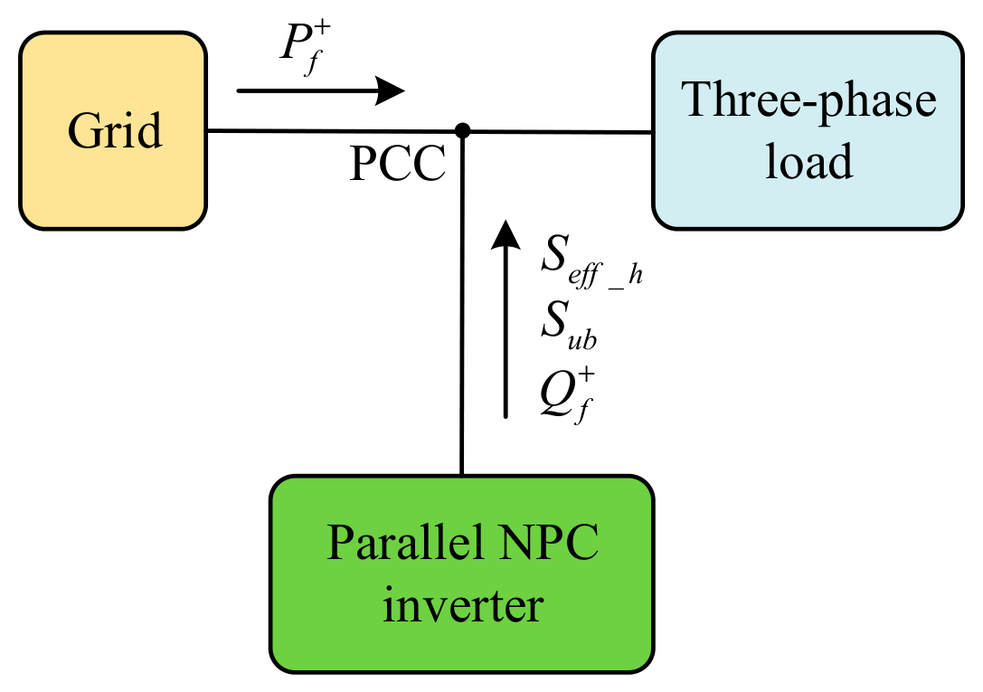
Only the power flow in the compensated system as V⁺_f at PCC is considered, as shown in Figure 1. The grid must provide all the power consumed by the load P⁺_f, Q⁺_f, S_ub and S_{eff_h} without shunt inverter. Otherwise, only P⁺_f flows out of the grid and the rest of the power is provided by the shunt inverter. When the shunt inverter is operated under non-ideal voltage conditions, S_{eff_h} and a part of S_ub are delivered by the grid. In both cases, only I⁺_Lf is supplied by the grid and the efficiency of the power system is maximized. The power quantities and power quality analysis in this section follow IEEE Standard 1459-2010 [25].

3. System Configuration and Active Power Flows

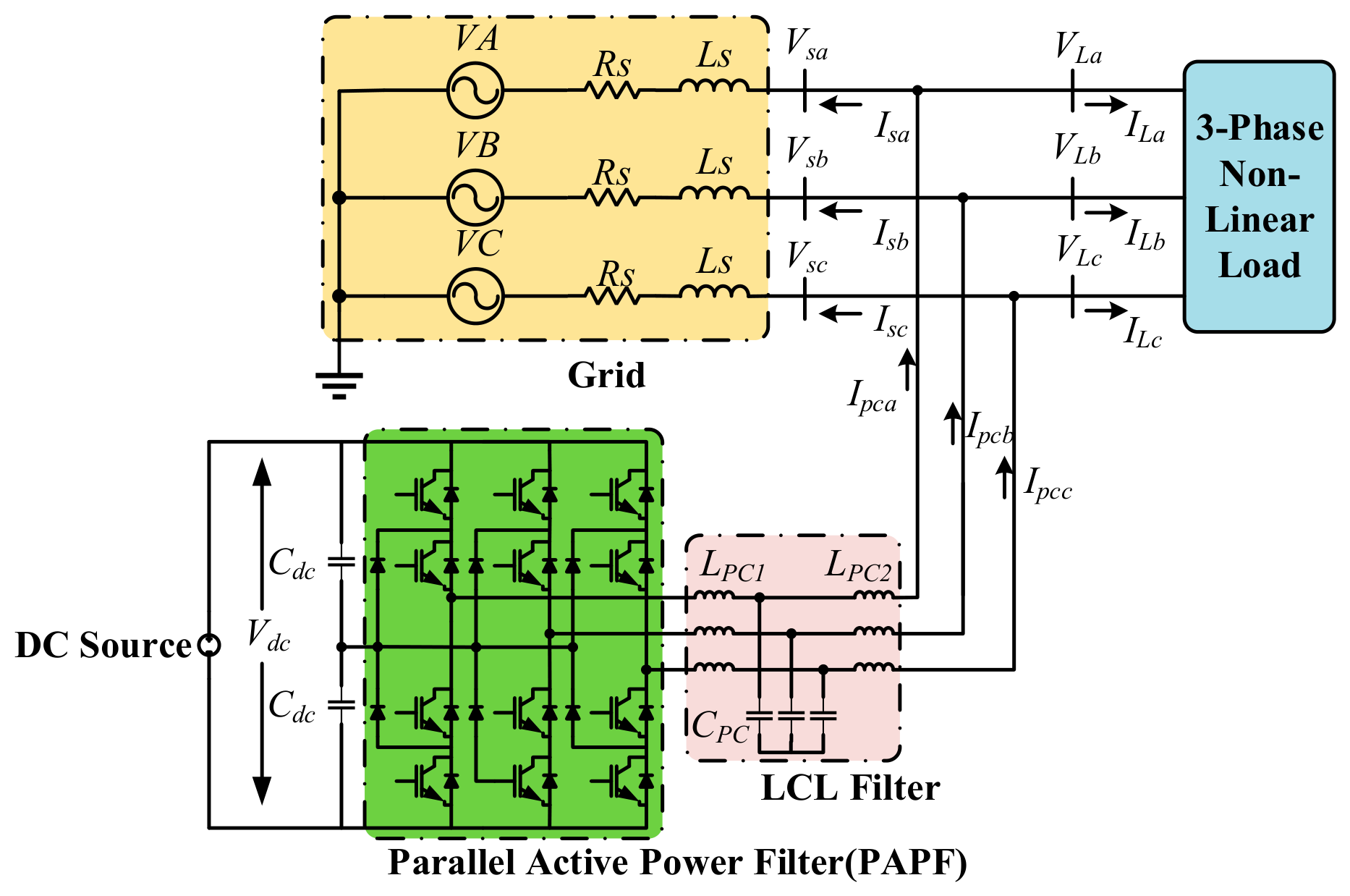
The system shown in Figure 2 primarily consists of two major subsystems, i.e., Parallel Active Power Filter (PAPF) and the DC bus. The PAPF consists of a three-level NPC (Neutral Point Clamped) inverter which is connected to PCC through inductance L_PC1, L_PC2, and capacitance C_PC. LCL filters are used to mitigate the harmonics generated by the high frequency switching. The DC bus is composed of the capacitors C_dc connected in parallel with the DC source.

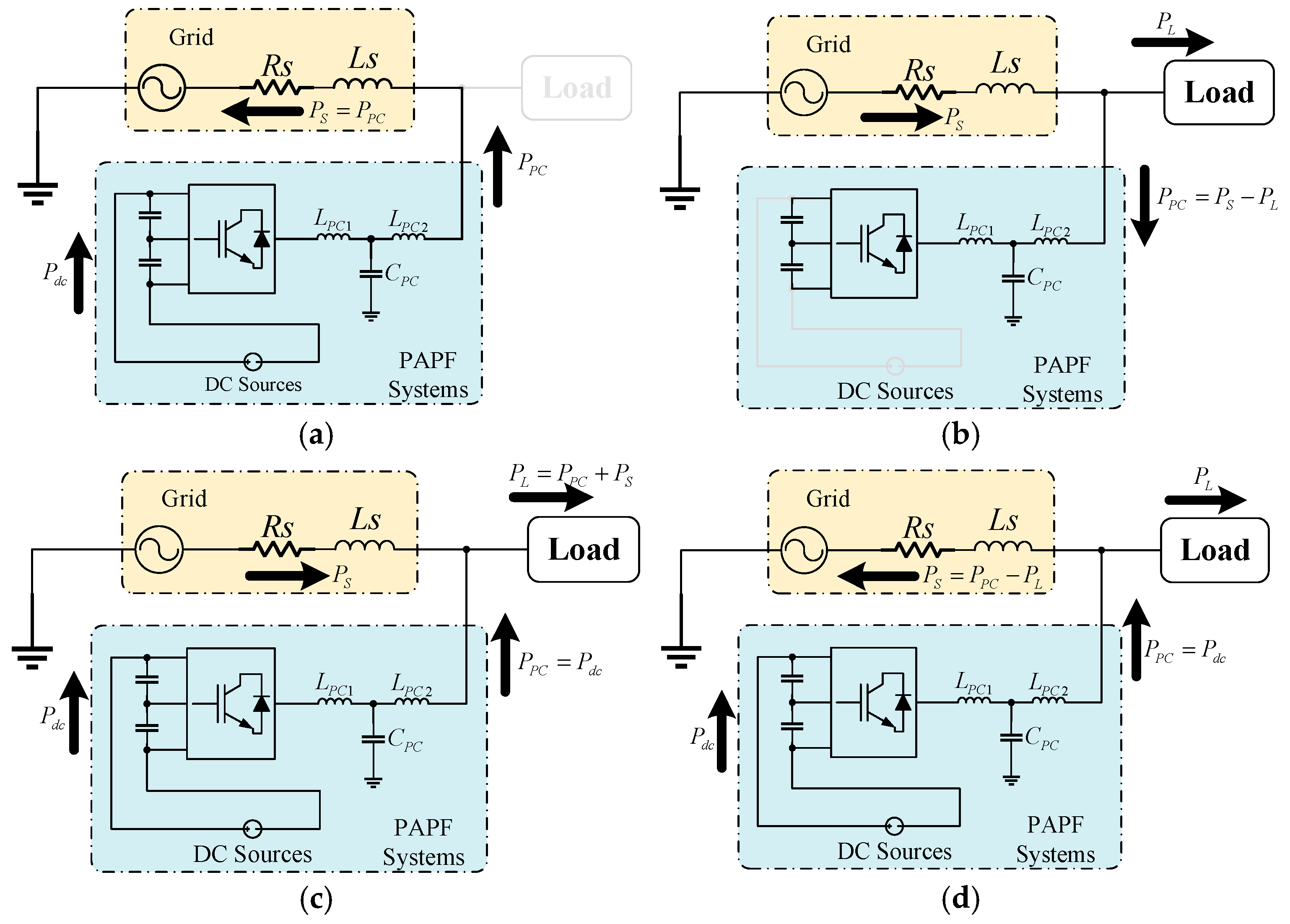
The power transfer characteristics of the PAPF system are theoretically analyzed, focusing on the instantaneous active power distributions, as illustrated in Figure 3. The flow of grid active power P_s, output active power of DC bus P_dc, shunt inverter active power P_PC, and load power P_L are schematically addressed. The operating conditions used to determine the active power flow are listed in

Table 2. Conditions of active power flow profile of PAPF system.

Operating Condition	Required Active Power of The Load	Output Active Power from DC Bus
1	PL = 0	Pdc ≠ 0
2	PL ≠ 0	Pdc = 0
3	PL ≠ 0	Pdc < PL
4	PL ≠ 0	Pdc > PL

.

Figure 3a shows the power flow through the PAPF in a zero-load condition (P_L = 0). In this case, the shunt NPC inverter will absorb all P_dc and P_PC = P_dc. All the active power is injected into the grid (P_S = P_PC). The power flow of case with P_L ≠ 0 and P_dc = 0 is shown in Figure 3b. The shunt NPC inverter is unable to provide active power. The grid-side starts to power up (P_S), which provides sufficient active power (P_L) to the loads and the rest power (P_PC = P_S − P_L) flows to the shunt inverter. Then it becomes a purely grid-powered condition. The case with P_L ≠ 0, P_dc ≠ 0, P_L > P_dc is shown in Figure 3c; the shunt NPC inverter preferentially transmits all the active power P_dc, i.e., P_PC = P_dc, which leads to insufficient power demand for load when P_L > P_dc. Then the grid power P_S is activated to keep the system power-balanced and the required power of load is achieved with P_L = P_S + P_PC. This case is the hybrid supply-insufficient power condition. In Figure 3d, both load and DC source are connected to the system (P_L ≠ 0, P_dc ≠ 0), and P_dc = P_PC. Since P_L < P_dc, the shunt inverter not only feeds the required load power (P_L), but also injects the remaining power into the grid (P_S = P_PC − P_L). This is the hybrid supply-sufficient power condition.

4. Automated Transition Strategy of Multifunctional PAPF System

The multifunctional PAPF control is mainly designed in a parallel NPC inverter and DC bus; the automated capacity-allocating-based transition strategy between harmonic and reactive power compensation is proposed from different perspectives. The detailed explanation of these subsystems is elaborated as follows.

4.1. Capacity-Allocating-Based Control of DC Bus

4.1.1. Active Power Control Algorithm of DC Bus

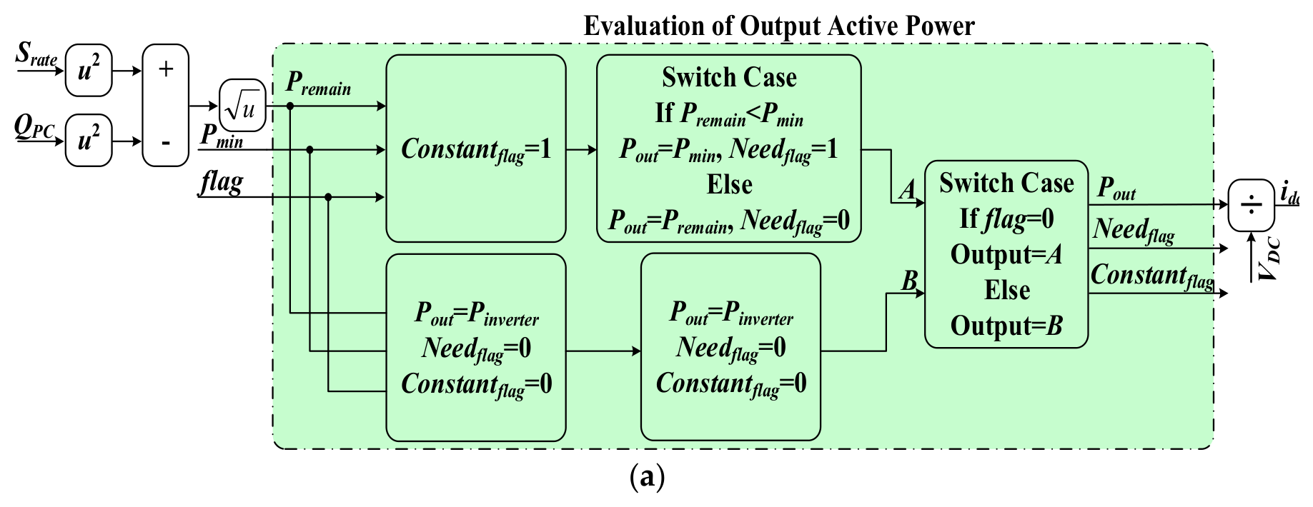
The main function of this part is to determine the minimum active power P_min required from the DC bus such that the grid current THD satisfies the IEEE-519 limit (THD_grid ≤ 5%), while respecting the rated capacity S_rated of the PAPF inverter. The algorithmic control flow of the DC bus is presented in Figure 4.

The equation to obtain DC-side current i_dc is shown below:

$$i_{dc}={\displaystyle \frac{P_{out}}{V_{dc}}}$$

(14)

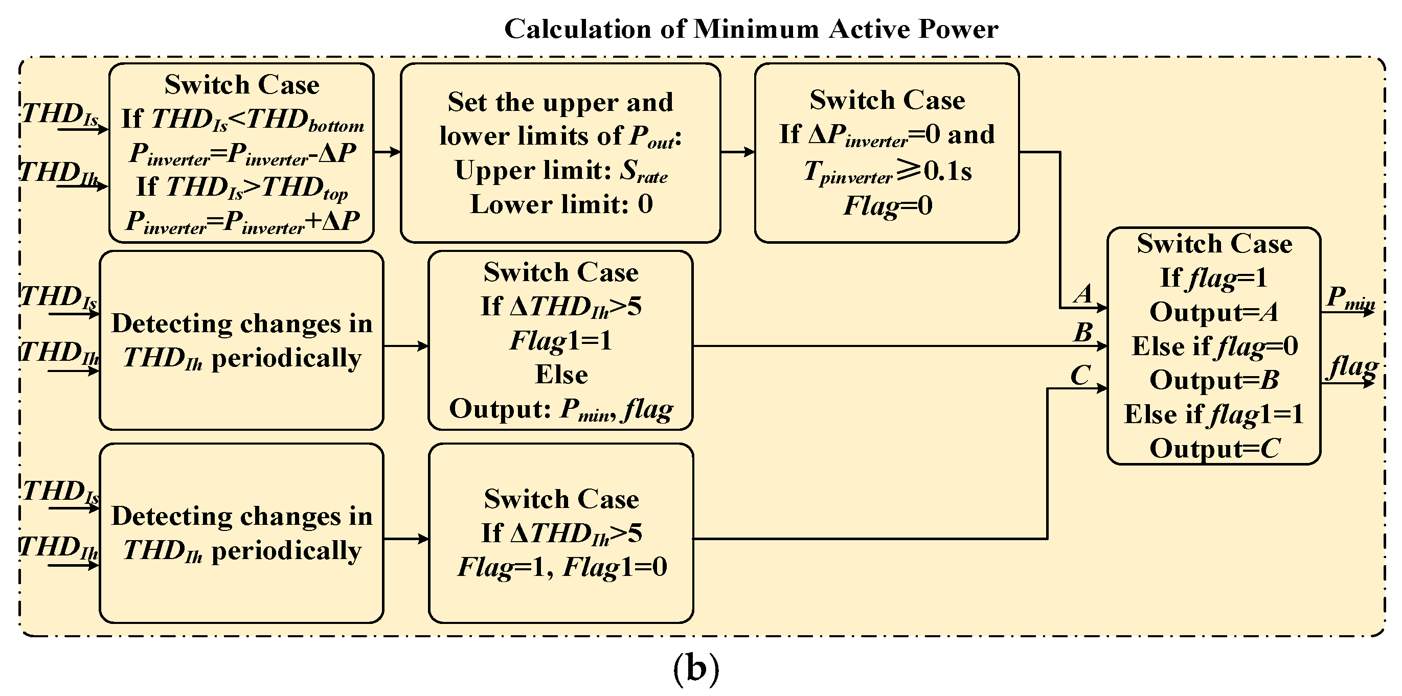
where P_out is the active power extracted from V_dc-DC bus. As it is connected to the battery, its charging/discharging current is dominated by the active power. As shown in Figure 4, the active power control consists of two parts: calculation of minimum active power and evaluation of output active power.

Instead of heuristic threshold comparisons, the minimum active power is defined as the solution of the following constraint satisfaction:

$$P_{\min }=min\left\{P_{out}\right|TH{D}_{grid}(P_{out})\le TH{D}_{\max }\}$$

(15)

The recalculation of P_min is event-triggered only when the harmonic content of the load current changes significantly (detected by a change in THD_load). If only the fundamental load power varies while the harmonic spectrum remains unchanged, P_min is not recalculated. This avoids unnecessary transients. The procedure is illustrated in Figure 4. Two flag signals, flag and flag1, are the event-detector labeling. flag is used to choose between minimum active power calculation and the load-change detection, and flag1 is used to clarify the reason for load change. As the inputs of minimum active power calculation, THD_Is is the grid current THD, and THD_Ih is the THD of load harmonic current. The active power extracted from the DC bus is controlled at the rated capacity, P_inverter. The calculation of the minimum active power is carried out until THD_Is is stabilized within THD_buttom to THD_top and P_inverter is unchanged.

Evaluation of output active power is conducted during the nonlinear load change, which is designed in event-trigger mode by detecting load harmonic THD periodically. The reason analysis is triggered once there is a disturbance in THD. Insufficient active power extracted from the PAPF inverter will result in poor harmonic compensation under the same load harmonic condition. There is one case with changed THD needs to be specified, i.e., the load with varied fundamental and unchanged harmonic component. It can be explained as purely load-power adjustment instead of load composition variation. Minimum active power does not need to be recalculated at this time.

Subsequently, the evaluation of the output active power is enabled. The remaining capacity of the PAPF after allocating P_min is:

$$P_{remain}=S_{rated}-\sqrt{P_{min}^2+Q_{PC}^2}$$

(16)

where Q_pc is the reactive power already compensated by the PAPF. The condition for safe harmonic compensation is P_remain ≥ 0. If this is violated, the reactive power compensation is reduced. P_inverter is constantly adjusted, and Need_flag provides the performance evaluation of harmonics compensation; even load reactive power compensation is implemented in parallel. Constant_flag is used to detect whether the reactive power compensation is terminated during calculating minimum active power. Meanwhile, the load reactive power is compared to P_remain and P_min. If P_remain < P_min, the harmonic compensation has been affected by the compensation of load reactive power. P_min is released to satisfy harmonic compensation in priority. The remaining capacity P_remain, minus the power consumed by load reactive power compensation, is served for active power transfer. Finally, i_dc is derived through DC-bus power control and added to the PAPF inverter control.

4.1.2. Threshold Selection and Sensitivity Analysis

The upper and lower THD limits are selected as THD_top = 4.5% and THD_bottom = 3.5%. The upper limit is set 0.5% below the IEEE-519 limit of 5% to provide a safety margin against measurement noise and transient overshoots. The lower limit is set 1% below the upper limit to create a hysteresis band, preventing frequent toggling of the allocation logic when the grid current THD oscillates near a single threshold.

To evaluate the sensitivity of the proposed strategy to threshold selection, a parameter sweep was conducted under nominal load conditions (OPM I). THD_top was varied from 4.0% to 5.0% in steps of 0.2%, and THD_bottom was varied accordingly to maintain a 1% hysteresis band. Based on the measured data, the steady-state grid current THD remained below 5% in all cases, and the number of P_min recalculations per minute varied by less than 15%. This confirms that the strategy is robust against reasonable variations in threshold values.

For noise immunity, the event-trigger mechanism recalculates P_min only when a sustained change in THD_load is detected over five consecutive sampling cycles (5 × 100 μs = 0.5 ms). Additionally, a moving average filter with a window length of 10 sampling cycles (1 ms) is applied to THD_load. Under simulated noisy grid conditions (additive white Gaussian noise, SNR = 30 dB), no false triggering of the event detector was observed, and the grid current THD remained below 5%.

4.2. Multifunctional Control Algorithm of Parallel Active Power Filter

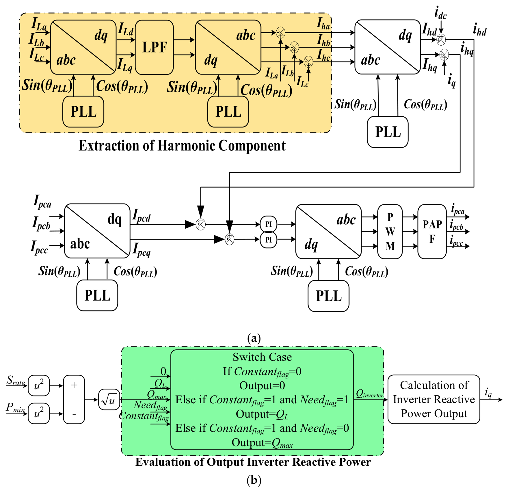
The PAPF operates under a strict lexicographic priority: harmonic compensation, which requires that the minimum active power P_min always be satisfied first; any remaining capacity is then allocated to reactive power compensation, and if capacity still exists, the excess active power is fed back to the grid. Harmonic compensation follows the conventional dq extraction and tracking method, while the novel aspect of the proposed strategy lies in the generation of the q-axis reference. Since it is operated in multifunctional mode, a smooth transition between harmonic and reactive power compensations is required in PAPF control. The harmonic compensation method contains two parts: harmonic component extraction and tracking. The harmonic detection process is shown in Figure 5a, where the load current is converted from abc to dq0 axis, and filtered out by a low-pass filter to obtain the fundamental component. The harmonic component is extracted by subtracting its original value after converting back to the abc axis. The harmonic compensation can be realized by injecting the harmonic components in the opposite direction into the grid. As shown in Figure 5, the reference of the PAPF output current I_pc is tracked by the PID controller. In harmonic component tracking, the component i_dc is introduced in the d-axis and i_q in the q-axis, wherein i_dc is used to control the active power of the DC bus, and i_q provides the reactive power control of the PAPF inverter.

The low-pass filter (LPF) used for harmonic extraction is a second-order Butterworth filter with a cutoff frequency of 50 Hz, which corresponds to a settling time (to 5%) of approximately 40–50 ms. This delay is typical for filtering-based harmonic detection methods and is acceptable for most industrial applications, as discussed in the transient analysis below.

Another control of the PAPF is to realize the reactive power compensation, including two parts: evaluation and calculation of output reactive power. The former is mainly determined by Need_flag, selector Constant_flag for Q_L and Q_max. Q_L is the reactive power required by load, and Q_max is the maximum reactive power to be compensated without degrading significant performance of harmonic compensation, which is obtained as follows:

$$Q_{max}=\sqrt{S_{rate}^2-P_{min}^2}$$

(17)

The actual commanded reactive power is then:

$$Q_{cmd}=min(Q_L,Q_{\max })$$

(18)

where Q_L is the load reactive power demand. Consequently, the q-axis current reference is:

$$i_q={\displaystyle \frac{Q_{cmd}}{V_{PCd}}}$$

(19)

The control diagram of reactive power output evaluation is shown in Figure 5b. Constant_flag is used to judge whether the minimum active power is being calculated. The automated transition between harmonic and reactive power compensation is managed through Need_flag. If the capacity is sufficient, Q_L will be fully utilized for the reactive power compensation. Otherwise, Q_L will be replaced by Q_max to solve the insufficient-capacity problem. Finally, the output reactive power of the PAPF, Q_inverter, is obtained and i_q is deduced as follows:

$$i_q={\displaystyle \frac{3V_{P{C}_q}\times I_{h_d}-2Q_{inverter}}{3V_{P{C}_d}}}$$

(20)

where V_PCd and V_PCq are the PAPF voltages in the dq0 axis and I_hd is the load current harmonic in the d-axis, respectively.

4.3. Stability Analysis of the PAPF Inverter

This subsection focuses on the stability analysis of the shunt NPC inverter when the load current changes. It can be summarized as follows:

$$\begin{array}{c}{\displaystyle \frac{I_{PC\_dq0}\left(s\right)}{I_{h\_dq0}\left(s\right)}}={\displaystyle \frac{X_1{s}^2+X_{2}s+X_3}{Y_1{s}^3+Y_2{s}^2+Y_{3}s+Y_4}}\end{array}$$

(21)

where:

$$\begin{array}{c}\left\{\begin{array}{l}{X}_1=W{K}_p{R}_C{C}_{PC}\\ X_2=W\left(K_p+K_i{R}_C{C}_{PC}\right)\\ X_3=K_i\\ Y_1=\left(L_{PC1}+L_{PC2}\right)C_{PC}\\ Y_2=\left(R_{L1}+R_{L2}+W{K}_p{R}_C\right)C_{PC}\\ Y_3=W\left(K_p+K_i{R}_C{C}_{PC}\right)\\ Y_4= W{K}_i\\ W={\displaystyle \frac{V_{dc}}{2}}{K}_{pwm}\end{array}\right.\end{array}$$

(22)

K_p and K_i are the proportional and integral gains used by the PI controller in the current control loop, respectively, and K_pwm is the equivalent PWM gain of the parallel NPC inverter.

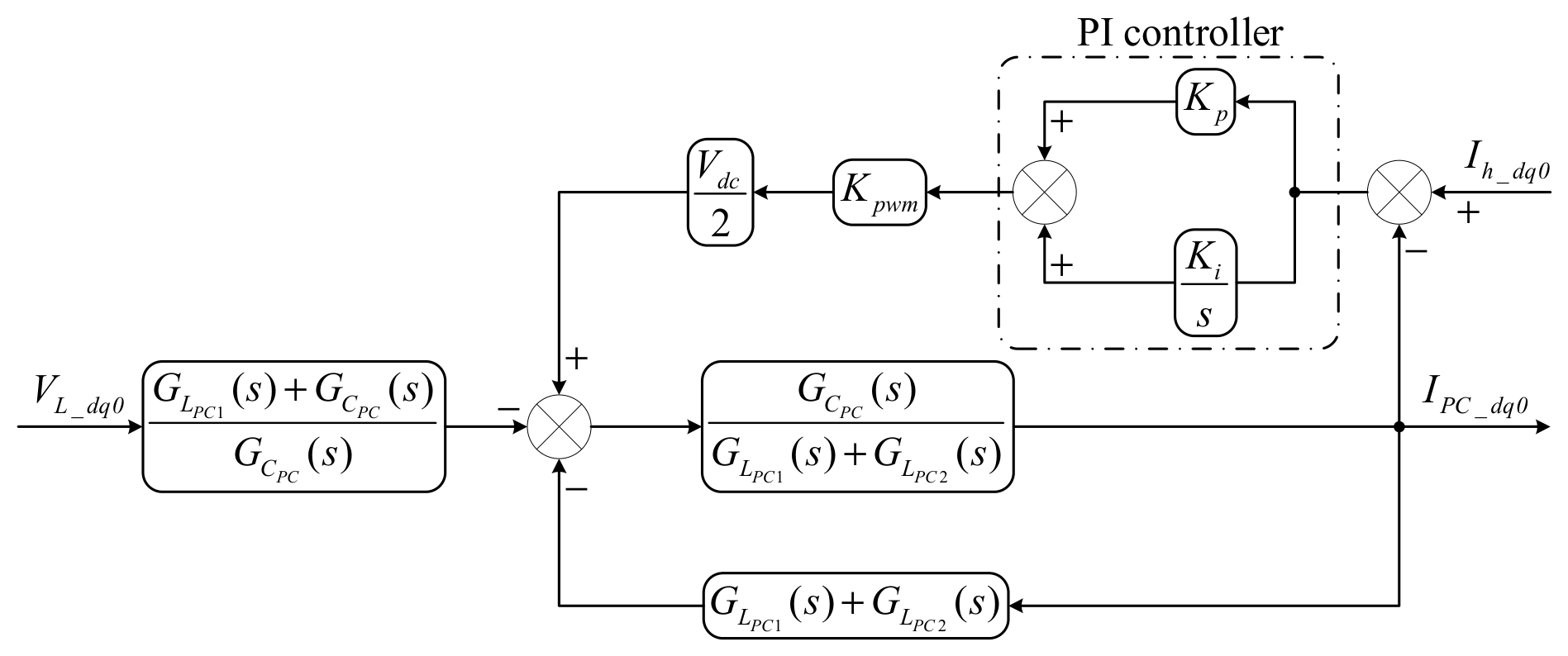
The control loop of the shunt NPC inverter is shown in Figure 6, where it is implemented in the dq0 axis on a synchronous rotating reference frame. Load voltage V_{L_dq0} is input and the shunt inverter current I_{PC_dq0} is output. The parasitic resistors R_L1 and R_L2 of the inductors, L_PC1 and L_PC2 in the LCL filter, the parasitic resistance R_C of the capacitor C_PC are taken into account to improve the analysis accuracy.

The transfer function as shown in Figure 6 can be obtained:

$$\begin{array}{c}{\displaystyle \frac{I_{PC\_dq0}\left(s\right)}{V_{L\_dq0}\left(s\right)}}={\displaystyle \frac{-\frac{G_{L_{PC1}}\left(s\right)+G_{C_{PC}}\left(s\right)}{G_{C_{PC}}\left(s\right)}s}{\left[\frac{G_{L_{PC1}}\left(s\right)+G_{L_{PC2}}\left(s\right)}{G_{C_{PC}}\left(s\right)}+G_{L_{PC1}}\left(s\right)+G_{L_{PC2}}\left(s\right)+W{K}_p\right]s+W{K}_i}}\end{array}$$

(23)

where the transfer functions G_Lpc1(s), G_Lpc2(s) of the inductor L_PC1, L_PC2 and the transfer function G_Cpc(s) of the capacitor C_PC are denoted as:

$$\begin{array}{c}\left\{\begin{array}{c}{G}_{L_{PC1}}\left(s\right)=L_{PC1}s+R_{L1}\\ G_{L_{PC2}}\left(s\right)=L_{PC2}s+R_{L2}\\ G_{C_{PC}}\left(s\right)={\displaystyle \frac{1}{C_{PC}s}}+R_C\end{array}\right.\end{array}$$

(24)

Substituting (24) into (25), the final expression of I_PCdq0 (s)/V_Ldq0 (s) is obtained:

$$\begin{array}{c}{\displaystyle \frac{I_{PC\_dq0}\left(s\right)}{V_{L\_dq0}\left(s\right)}}={\displaystyle \frac{X_1^{\prime }{s}^3+X_2^{\prime }{s}^2+s}{Y_1^{\prime }{s}^3+Y_2^{\prime }{s}^2+Y_3^{\prime }s+Y_4^{\prime }}}\end{array}$$

(25)

where:

$$\begin{array}{c}\left\{\begin{array}{l}{X}_1^{\prime }=-L_{PC1}{C}_{PC}\\ X_2^{\prime }=-(R_{L1}{C}_{PC}+R_C{C}_{PC})\\ Y_1^{\prime }=C_{PC}\left(R_C+1\right)\left(L_{PC1}+L_{PC2}\right)\\ Y_2^{\prime }=C_{PC}\left(R_C+1\right)\left(R_{L1}+R_{L2}\right)+L_{PC1}+L_{PC2}+W{K}_p{R}_C{C}_{PC}\\ Y_3^{\prime }=R_{L1}+R_{L2}+W{K}_p+W{K}_i{R}_C{C}_{PC}\\ Y_4^{\prime }=W{K}_i\end{array}\right.\end{array}$$

(26)

The characteristic equation is further derived from (25):

$$\begin{array}{c}{Y}_1^{\prime }{s}^3+Y_2^{\prime }{s}^2+Y_3^{\prime }s+Y_4^{\prime }=0\end{array}$$

(27)

The coefficients in (27) are of the same sign and satisfy the inequality Y′₂Y′₃ > Y′₁Y′₄. It is observed that coefficients of Y′₁, Y′₂, Y′₃, and Y′₄ are greater than zero. Therefore, the Routh–Hurwitz stability criterion is satisfied by (27). In addition, the system can be stabilized by adjusting K_P and K_i appropriately. The load change only affects the current reference of the current control loop and there is no essential impact on system stability. This conclusion holds for all three operating modes under the proposed capacity allocating control, because the current control loop structure remains unchanged.

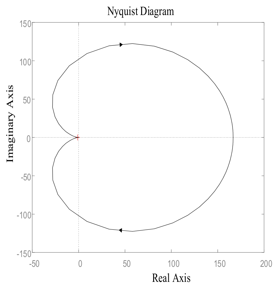
The Nyquist plot obtained from (25) is outlined in Figure 7. The change of the plot is potentially dependent on the filters, and the filter parameters are shown in

Table 3. Parameters adopted in the experiments.

Nominal RMS grid voltages	Vs = 127 V
Utility grid frequency	fs = 50 Hz
Inductive filters	LPC1 = 2.2 mH, LPC2 = 100 uH
Capacitive filters	CPC = 9.4 uF
Dc-bus equivalent capacitance	CDC = 1360 uF
Dc-bus voltage	Vdc = 600 V
PAPF rated capacity	Srate = 5500 VA
THD upper limit	THDtop = 4.5%
THD lower limit	THDbutton = 3.5%
Three-phase nonlinear loads
Bridge Rectifier with RL−L:LL = 1 mH
1. RL = 150 Ω, Introduction of reactive power 3000 VA, THD = 15.59%
2. RL = 150 Ω, Introduction of reactive power 3500 VA, THD = 13.88%
3. RL = 75 Ω, No introduction of reactive power, THD = 31.10%

, which is also designed as the experimental coefficients. As seen in Figure 7, there are no open-loop poles in the right-half plane, and the point (−1, j0) is not enclosed by the Nyquist curve. It is consolidated that the closed-loop system is stable. Therefore, the proposed automated transition strategy does not compromise system stability.

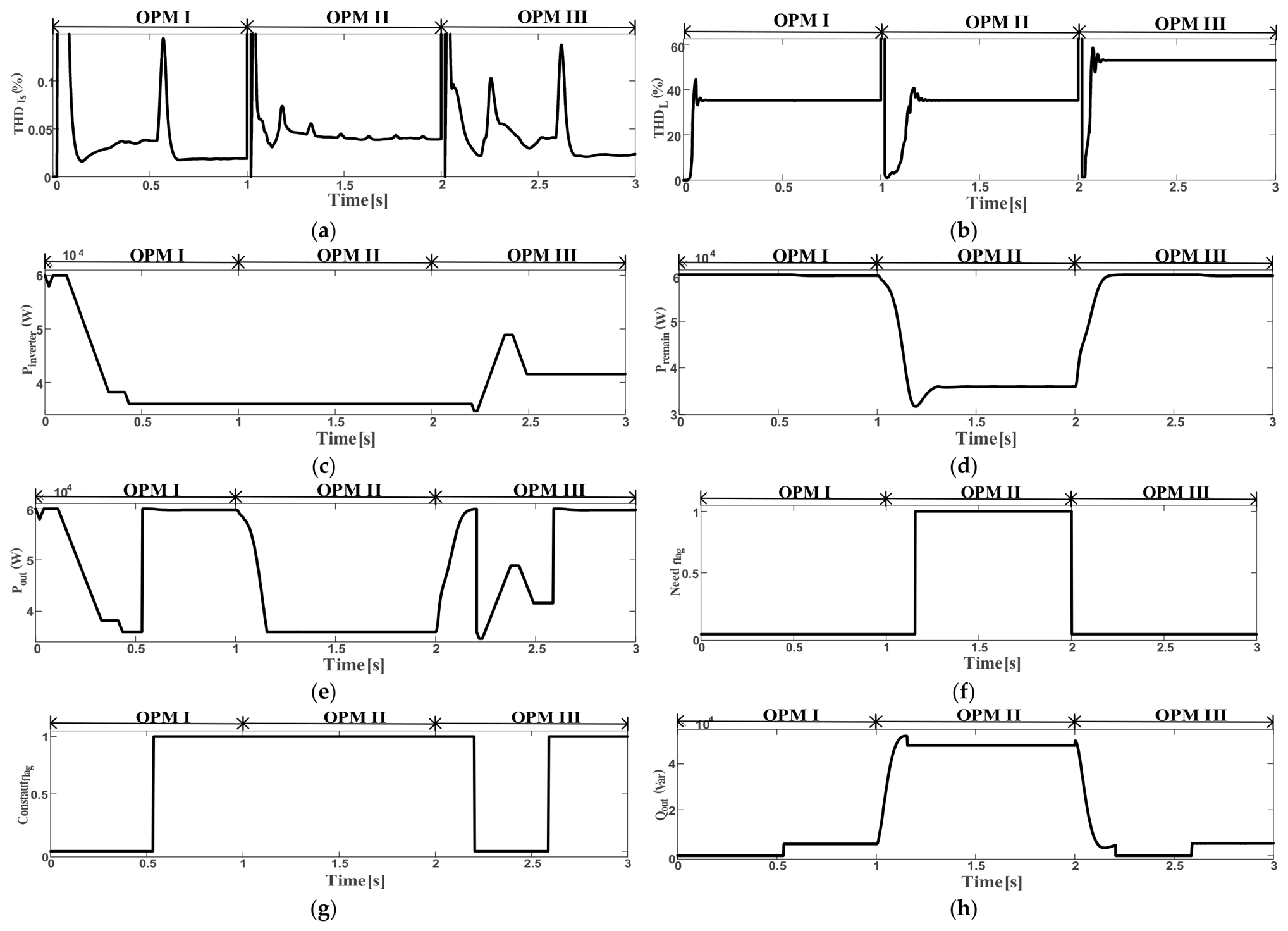
To further verify stability, we conducted transient simulations where the system undergoes abrupt OPM changes (I → II → III). As shown in Figure 8, the grid current THD remains below 5% during and immediately after each transition, and no sustained oscillations are observed. This confirms that the proposed automated transition strategy does not compromise system stability.

4.4. Comparison with an Optimization Baseline

To quantitatively evaluate the optimality gap of the proposed heuristic strategy, a simple offline linear programming (LP) problem is formulated. The objective is to maximize the reactive power compensation capacity Q_comp subject to the following constraints:

• Grid current THD ≤ 5% (IEEE-519 compliant);
• PAPF apparent power S_PAPF ≤ S_rated.

The required minimum active power P_min for harmonic compensation is obtained from the sweep results described in Section 4.1. The optimal reactive power Q_opt is then computed as Q_opt = min(Q_load, sqrt(S_rated² − P_min²)), which represents the maximum reactive power that can be compensated without violating the rated capacity or the THD limit.

The LP problem is solved offline using the same load conditions as in Section 4.3 (the simulation study).

Table 4. Optimality gap comparison between heuristic and offline LP solution.

OPM	Qopt (kVar)	Qheuristic (kVar)	Ratio (%)
I	5.12	4.91	95.9
II	48.7	44.9	92.2
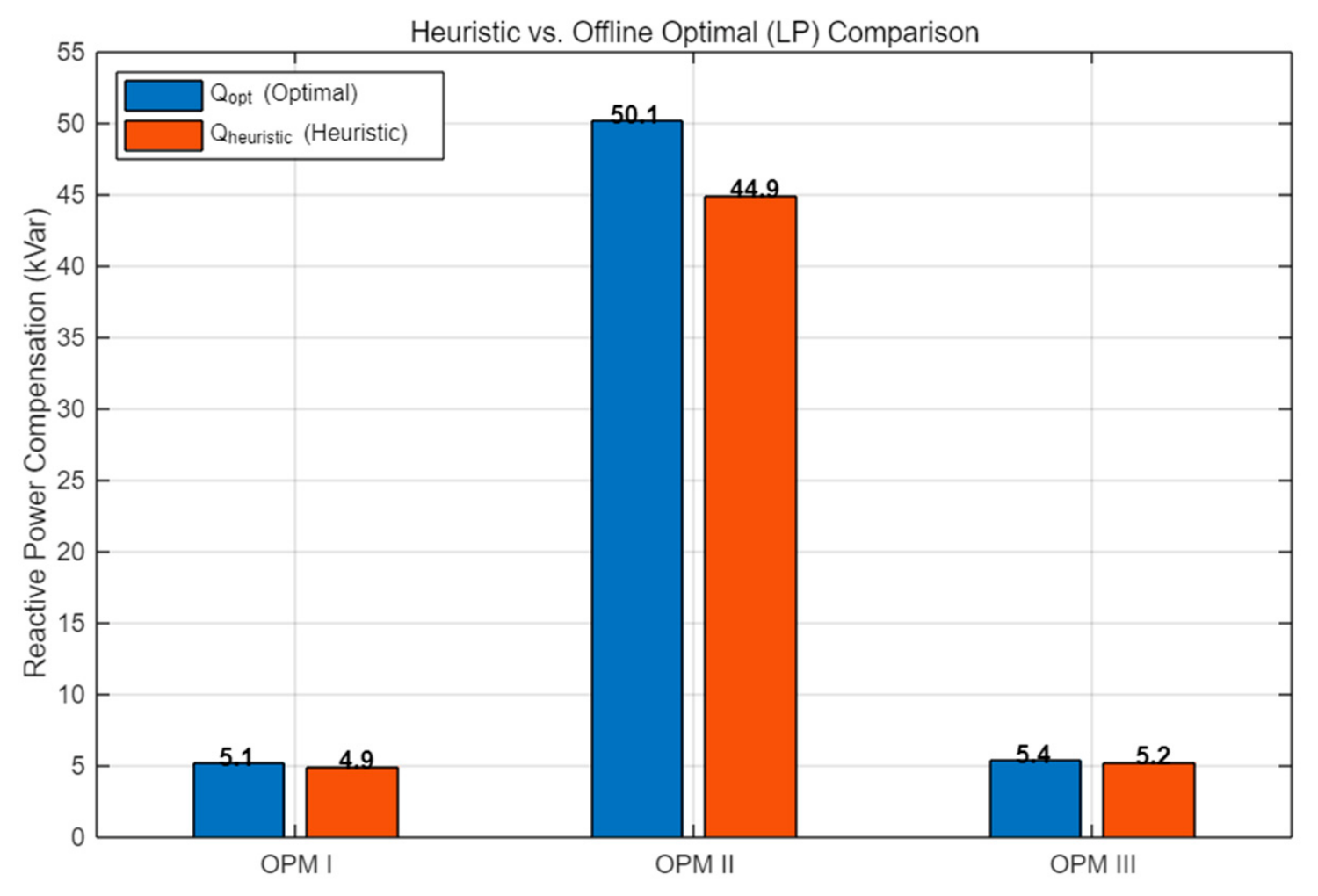
III	5.45	5.21	95.6

compares the optimal solution Q_comp with the actual reactive power Q_heuristic achieved by the proposed heuristic strategy in each operating mode. The results show that the heuristic strategy reaches 92–96% of the optimal performance across all three OPMs.

Figure 9 provides a visual comparison of the optimal and heuristic reactive power compensation capacities. The close alignment between the blue bars (optimal) and orange bars (heuristic) confirms that the proposed rule-based approach is near-optimal for the single-inverter scenario. More importantly, this near-optimal performance is achieved without any iterative computation and using only local measurements, making it highly practical for real-time DSP implementation.

5. Simulation Results

In this section, the proposed method is tested by numerical simulation using Simulink (R2026a) tool. The automated transition of this multifunctional PAPF system can be highlighted by three operating modes (OPMs), as described as follows.

(1)

OPM I: In OPM I, the required load reactive power is small and less than the maximum compensation value. In this case, a part of PAPF capacity is adopted to compensate the load reactive power and the rest is used to deliver the active power.

(2)

OPM II: In OPM II, the required load reactive power is large enough that it exceeds the maximum compensation value. In this case, harmonic compensation is operated in priority and the rest capacity of PAPF is used to compensate the load reactive power.

(3)

OPM III: In OPM III, the load harmonic component is changed due to its changing load impedance. In this case, the system restarts the minimum active power calculation and enters OPM I and OPM II as appropriate.

Based on the features of OPMs mentioned above, the load condition and power condition of each OPM can be mathematically summarized, as shown in

Table 5. Three OPMs of system operation <, => R_{L_OPM1}.

OPM	Load Condition	Power Condition
I	RL_OPM1	QL < Qmax, PPAPF > Qmax
II	RL_OPM2 = RL_OPM1	QL > Qmax, PPAPF < Qmax
III	RL_OPM3 < RL_OPM1	QL < Qmax, PPAPF > Qmax

.

The three OPMs are tested in the simulations. The rated capacity of the PAPF is defined as 60 kVA. The load is connected to a nonlinear load with reactive power of 5 kVar and THD is up to 59.11%. Firstly, the system starts to calculate P_min, and Constrant_flag and Q_out are initially 0, as seen in Figure 10g,h. During OPMI, P_inverter is resized according to THD_Is. P_inverter is increased if THD_Is is greater than THD_top and it is decreased when THD_Is is less than THD_buttom. As observed in Figure 10c, THD_Is is unstable but bounded between THD_buttom and THD_top at around 0.4 s. P_inverter is adjusted constantly until THD_Is has stabilized in the range of [THD_buttom, THD_top] at around 0.5 s. At the end of P_min calculation, the load reactive power compensation is activated and Constrant_flag converts to 1. All the remaining capacity of the PAPF starts to output active power, as shown in Figure 10e. In the OPM II test, the nonlinear load is changed so that a reactive power of 50 kVar is consumed and THD becomes 13.8%. Compared to OPM I, the required reactive power is increased, whereas the harmonic component remains unchanged. In this case, there is no need to recalculate P_min in Figure 10b. However, the required load reactive power exceeds the maximum threshold and Need_flag is set to 1. Only a part of reactive power is compensated by the PAPF system, and the remaining capacity, i.e., P_min, is adopted to compensate the harmonics. In OPM III, the nonlinear load with reactive power of 5 kVar and THD of 71.53% is designed. The difference between OPM I and OPM III exists in the harmonic component. P_min needs to be recalculated and the reactive power compensation is terminated. The capacity left is used to output active power until the end.

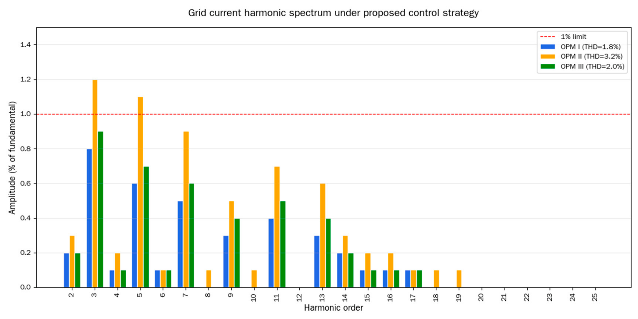
To further evaluate the harmonic suppression performance, Figure 11 presents the harmonic spectrum of the grid current under the proposed control strategy for OPM I, OPM II, and OPM III, respectively. The spectrum is shown up to the 25th order (2.5 kHz), which lies within the controller bandwidth. It can be observed that the dominant harmonic components (5th, 7th, 11th, and 13th) are all suppressed to below 1% of the fundamental in all three operating modes. This detailed spectral analysis confirms that the low grid current THD (consistently below 5%) is achieved by effective attenuation of the major harmonics, rather than by masking them through a high fundamental component.

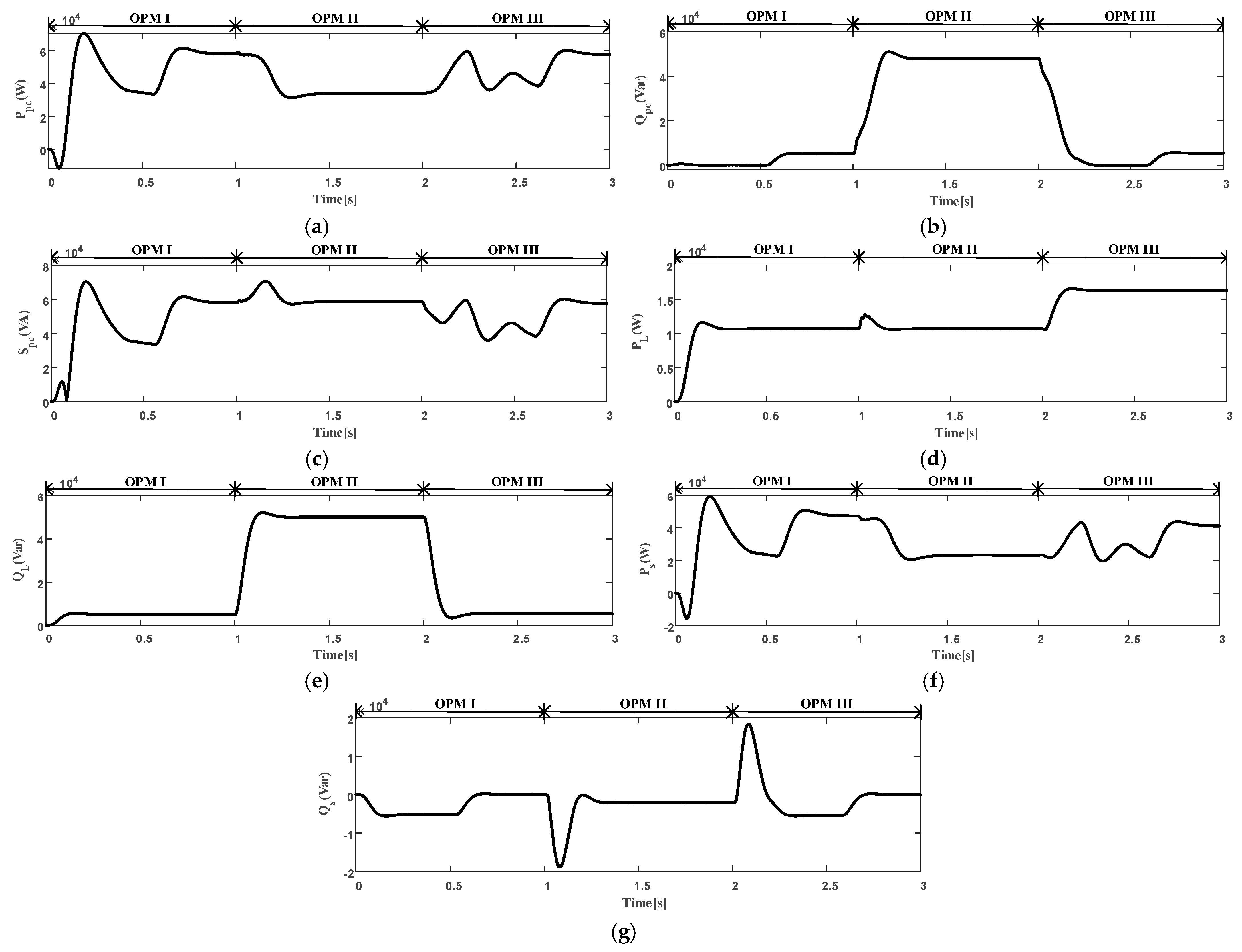
The reactive power Q_pc generated by PAPF system plays the role of compensation on load reactive power Q_L. The load side can be compensated through the power grid by a little reactive power output, as shown in Figure 12g. In addition, the apparent power flowing through the PAPF at steady state is within the rated capacity, which protects and makes full utilization of the inverter, as addressed in Figure 12c. The performance of harmonic compensation is shown in

Table 6. Average THD value of grid current for three OPMs.

OPM	THDIs%
I	1.87
II	3.98
III	2.29

. It is emphasized that the harmonics is effectively compensated and the THD value of grid current I_s is restricted to 5% in the three OPMs.

To provide a more detailed harmonic analysis beyond the overall THD values, Figure 12 presents the harmonic spectrum of the grid current under the proposed control strategy for OPM I, OPM II, and OPM III (up to the 25th order). The dominant harmonic components (5th, 7th, 11th, 13th) are all suppressed to below 1% of the fundamental, which explains why the overall THD remains below 5% in all cases.

Furthermore,

Table 7. Harmonic suppression comparison: load current (uncompensated) vs. grid current (compensated) under the proposed strategy.

Harmonic Order	Uncompensated Load Current (%)	OPM I (Compensated, %)	OPM II (Compensated, %)	OPM III (Compensated, %)
5th	28	1.2	2.1	1.4
7th	18	0.8	1.5	0.9
11th	9	0.5	0.9	0.6
13th	6	0.3	0.7	0.4
Others (average)	~5.0	≤0.3	≤0.4	≤0.3
Total THD	~59% (per Table 2)	1.87% (Table 6)	3.98% (Table 6)	2.29% (Table 6)

quantifies the harmonic suppression performance by comparing the individual harmonic magnitudes of the uncompensated load current and the compensated grid current under the proposed strategy. Taking OPM I as an example, the 5th harmonic is reduced from 28% to 1.2%, and the 7th harmonic is reduced from 18% to 0.8%. Similar reductions are observed for the 11th and 13th harmonics. This quantitative breakdown demonstrates the effectiveness of the proposed strategy beyond just the overall THD number.

6. Experimental Results

6.1. Conclusions and Contributions

The performance of the three-phase PAPF was evaluated through prototype tests in the three OPMs: the rated capacity of the PAPF is sufficient for both harmonic and reactive compensation, insufficient for reactive compensation, and there is a change in load harmonic component. The experimental parameters are presented in Table 2 The sinusoidal pulse width modulation (SPWM) technique was adopted in the NPC PAPF inverter.

In the experimental implementation, the control algorithm is executed on a TMS320F28335 DSP (Dallas, TX, USA) operating at 150 MHz. The sampling frequency is set to 15 kHz (sampling period Ts = 100μs), and the switching frequency of the SPWM carrier is 15 kHz. The PI controller gains are tuned as \(K_p = 2.5\), \(K_i = 50\) for the inner current control loop, and \(K_p = 0.8\), \(K_i = 20\) for the voltage/power regulation loop.

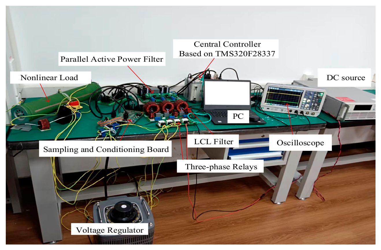
The laboratory prototype of the developed system is shown in Figure 13. The control is implemented using DSP TMS320F28335. The performance of the three-phase PAPF with three-level NPC topology under different OPMs has been investigated. The test results are detailed below.

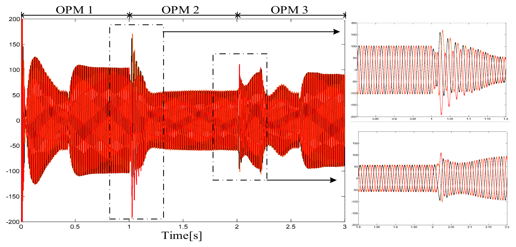
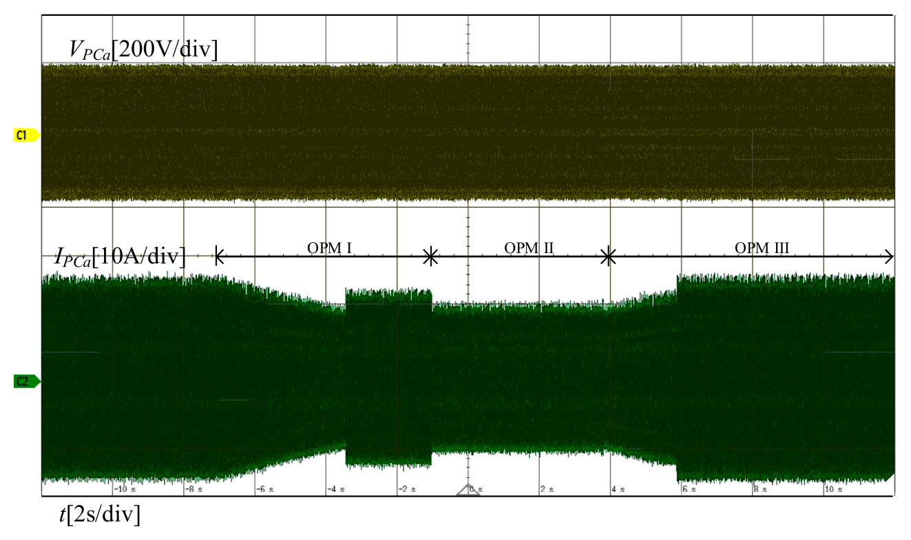
The overall process of the experiment involving OPM I/II/III is presented globally in Figure 14. At the beginning, the control algorithm is not activated and there is no load reactive power compensation yet. The calculation of minimum active power is enabled when the system is running in OPM 1, which is reflected by the decreasing output current, “a” phase of I_pc, as shown in Figure 14. The system starts compensating reactive power and uses the remaining capacity of PAPF to transfer active power. The amplitude of the PAPF output current is less than the initial value due to the energy consumption to deliver reactive power. When the reactive power required by the load is increased so that it exceeds the maximum compensation capacity allowed by PAPF, the output current amplitude of PAPF can only be maintained at the level shown in Figure 14 no matter how much the consumed load reactive power is increased, which is a feature of OPM II. In the OPM III test, the resistance in nonlinear load is reduced by half, resulting in an increase in both the harmonic component and the minimum active power. The calculation of minimum active power is thereby triggered. As shown in Figure 14, the PAPF output current is increased until the updated minimum active power is obtained.

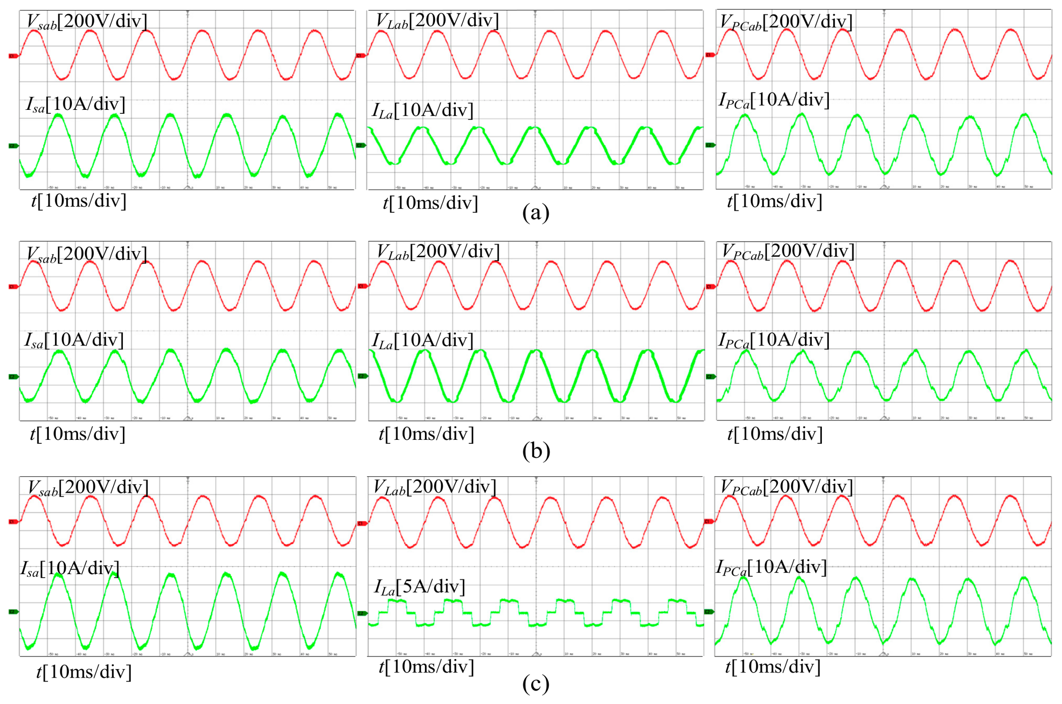
The experimental results involving voltages and currents of the grid, PAPF, load in the three OPMs are presented in Figure 15, respectively. The active and reactive power of the PAPF and load, THD of the grid current are recorded in

Table 8. Experimental data of power and THD sampled from ‘A’ phase.

PPC/W	QPC/Var	SPC/VA	PL/W	QL/Var	THDIS/%
OPM I
4505	2707	5256	468	3000	3.68
OPM II
4021	3384	5256	468	3571	4.59
OPM III
5256	84	5256	875	46	3.1

. It can be obtained that the automated transition between the reactive power and harmonics compensation at PAPF’s rated capacity in different OPMs is effectively realized. Moreover, the THD of the grid current is restricted to below 5% during the entire compensation process.

To further demonstrate the advantage of the proposed strategy, a quantitative comparison with the conventional global compensation (UPF method) is conducted based on the simulation results presented in Section 5. As summarized in

Table 9. Comparison between proposed and conventional (UPF) methods.

Method	Grid Current THD	PAPF Apparent Power	Rated Capacity Violation
Conventional (UPF)	2.73% (OPM I)/2.86% (OPM II)	Exceeds rating in OPM II	Yes
Proposed	<5% in all OPMs	Within rating	No

, the conventional UPF method achieves low grid current THD (2.73% in OPM I and 2.86% in OPM II) but violates the rated capacity under high reactive power demand (OPM II). In contrast, the proposed strategy maintains the grid current THD below 5% in all operating modes while keeping the PAPF apparent power strictly within the rated capacity. This confirms that the proposed method effectively resolves the conflict between compensation depth and rated capacity limitation.

6.2. Future Work: Extension to Multi-Inverter and AI-Based Allocation

While the proposed heuristic strategy is effective for a single PAPF operating at its rated capacity, many practical scenarios involve multiple inverters (e.g., multiple PAPFs or grid-forming inverters with power quality services) sharing a common point of coupling. In such multi-inverter systems, the total inverter capacity becomes a scarce and valuable resource that must be allocated across competing services (harmonic mitigation, reactive support, active power curtailment, etc.) in a coordinated manner. A rule-based priority strategy may be insufficient to achieve global optimality, especially when economic incentives, communication delays, and fault tolerance are considered.

Therefore, future work will focus on:

• Multi-objective optimization: Formulating the capacity allocation as a Pareto optimization problem to trade off between multiple power quality indices (THD, power factor, voltage support) and economic objectives (e.g., revenue from reactive power market).
• AI-based allocation: Using reinforcement learning or deep Q-networks to learn near-optimal allocation policies under dynamic grid conditions and uncertain load profiles.
• Distributed coordination: Developing consensus-based or primal-dual algorithms for multi-inverter coordination without a central controller.

A preliminary simulation of a two-PAPF system is presented below as an illustrative preview. The experimental platform developed in this paper provides a solid foundation for validating these advanced allocation strategies in future work.

7. Conclusions

An automated capacity-allocating-based transition strategy of multifunctional PAPF was proposed in this paper. By calculating the minimum active power and evaluation of the active/reactive power, the continuous compensation of reactive power to the loads, without affecting the performance of harmonic compensation, is realized. This reduces the reactive power flowing to the load and improves the power factor on the grid. In addition, the power distribution limits the power flowing through the PAPF so that the total amount of power is kept at the rated capacity level. As a result, safe operation is guaranteed and the utilization rate of the PAPF device is enhanced. The behavior of the system in terms of harmonics and reactive power compensation was found to be satisfactory and the grid currents met the THD limits prescribed in the IEEE-519 standard [26].

The response of the multifunctional PAPF was extensively evaluated under three OPMs; we found high reliability under the changing conditions of load. Meanwhile, the multifunctional PAPF can distribute the active and reactive power appropriately according to the load disturbances. Moreover, the system operates well in automated transition between different operating modes and shows that it adapts to the varied nonlinear loads effectively. Future work will focus on reducing the harmonic detection delay using predictive algorithms (e.g., Kalman filters or adaptive notch filters) to further improve the transient response for extremely sensitive loads or weak grid conditions.