Static Voltage Stability Assessment of Renewable Energy Power Systems Based on DBN-LSTM Power Forecasting

Abstract

High penetration of renewable energy sources (RESs) introduces significant power fluctuations, threatening voltage and frequency stability in modern power systems. This paper presents an integrated framework for static voltage stability assessment and stability-constrained optimization of under-frequency load shedding (UFLS) in renewable-dominated grids. A low-conservativeness analytical criterion is first derived for static voltage stability margin assessment. Then, a hybrid Deep Belief Network–Long Short-Term Memory (DBN–LSTM) model is developed for accurate renewable power forecasting, capturing temporal variability and uncertainty. Finally, UFLS-based stability-constrained dispatch is formulated to prevent voltage collapse, enhance the system stability, and minimize RES curtailment. Simulations on a modified IEEE benchmark system demonstrate that the proposed approach improves voltage and frequency stability while maintaining high renewable energy utilization.

1. Introduction

With the increasing penetration of renewable energy sources (RESs) in power systems, the operational complexity of modern power grids has significantly increased. Due to the inherent intermittency and stochastic characteristics of renewable generation, fluctuations in power output lead to continuous variations in system power injections, driving operating points closer to voltage stability limits. Static voltage stability reflects the ability of a power system to maintain a feasible equilibrium operating point under steady-state conditions. However, as the penetration level of renewable energy continues to grow, traditional stability analysis methods based on deterministic assumptions become increasingly inadequate for accurately characterizing system operating states. Therefore, under highly uncertain operating environments, effective analytical methods and stability criteria are required to quantify system stability margins.

Research on explicit analytical conditions for static voltage stability has a long history. Early studies by Wu and Kumagai [1] and Ilić [2] derived sufficient conditions for the solvability of transmission system power flow equations. These ideas were later extended to distribution networks by Chiang and Baran [3] and Miu and Chiang [4], who investigated the existence and uniqueness of power flow solutions. In recent years, advanced mathematical tools such as energy function methods and monotone operator theory have been introduced to characterize convex security regions that guarantee power flow solvability [5,6]. For simplified decoupled power flow models on acyclic networks, Dörfler et al. [7] established necessary and sufficient conditions for solution uniqueness, which were later strengthened by Jafarpour and Bullo using the cutset projection operator [8]. More recently, Jafarpour et al. [9] proposed a unified topological framework on the n-torus to analyze network solvability, providing both uniqueness guarantees and convergent iterative algorithms, with subsequent extensions to lossy systems [10]. Despite these theoretical advances, the resulting analytical conditions are often conservative and may underestimate the actual solvability region of the system. Moreover, although similar analyses have been conducted for reactive power flow and DC networks [11,12,13], results for fully coupled AC models remain largely limited to small-scale systems such as two-bus networks [14]. These limitations highlight the need for more practical stability assessment approaches for large-scale power systems with high renewable penetration.

As renewable energy introduces significant uncertainty into system operation, deterministic voltage stability analysis becomes insufficient for representing real operating conditions. Consequently, probabilistic voltage stability assessment methods have been developed by explicitly modeling uncertainties in renewable generation and load demand. Existing approaches can generally be categorized into sampling-based probabilistic power flow methods and statistical distribution-based modeling methods. Monte Carlo Simulation (MCS) combined with Continuation Power Flow (CPF) is widely used in sampling-based approaches. Alzubaidi et al. [15,16] employed an MCS–CPF framework to analyze the impacts of load models, reactive power reserves, and wind generation control modes on voltage stability margins. Their results showed that renewable generation variability significantly alters system stability boundaries. However, such methods require extensive sampling and repeated power flow calculations, leading to high computational costs and limiting their applicability for real-time stability assessment. To better capture correlations among uncertain variables, statistical modeling approaches have also been proposed. Huang and Yan applied Kernel Density Estimation (KDE) to derive probability density functions of wind speed and solar irradiance, and further employed Copula functions to construct joint probability distributions among stochastic variables. Combined with Quasi-Monte Carlo (QMC) sampling, this approach improves computational efficiency while preserving correlation characteristics [17]. Nevertheless, as the number of uncertain variables increases, the parameter estimation and joint distribution construction of Copula-based models become increasingly complex, which may limit their applicability in large-scale systems.

To improve computational efficiency and prediction accuracy, data-driven approaches have been increasingly explored for forecasting renewable generation and load demand. Because these variables exhibit strong nonlinear and temporal characteristics, traditional statistical forecasting methods often struggle to capture such complex dynamics. Consequently, machine learning and deep learning techniques have gained growing attention in recent years. Dong et al. [18] applied a support vector machine enhanced with K-means clustering for short-term load forecasting, achieving improved prediction accuracy at the expense of increased computational complexity. Veeramsetty et al. [19] combined Gated Recurrent Units (GRUs) with Random Forests to simultaneously capture temporal dependencies and reduce input dimensionality. Xiang et al. [20] further improved forecasting performance by incorporating multi-factor features such as meteorological and economic variables. Duan et al. [21] integrated modal decomposition with an optimized Long Short-Term Memory (LSTM) network to reduce forecasting errors and improve model robustness. Kim et al. [22] proposed advanced feature extraction methods for multivariate time-series forecasting, achieving significant reductions in RMSE. More recently, Jiang et al. [23] introduced a hybrid hierarchical deep learning framework that outperformed conventional forecasting approaches, while Zufferey et al. [24] developed a probabilistic multivariate forecasting model balancing prediction accuracy, uncertainty modeling, and computational efficiency. Despite these advances, challenges remain in fully exploiting deep feature learning for long-sequence load data and reducing the computational burden of complex deep learning models.

In addition to stability assessment, system protection schemes are widely employed to maintain secure power system operation under severe disturbances. Among them, under-frequency load shedding (UFLS) is an essential protection strategy designed to prevent frequency collapse and large-scale blackouts. With ongoing deregulation in power systems, many networks operate with reduced reserve capacity and smaller stability margins, increasing the risk of cascading failures [25]. UFLS is therefore one of the most widely adopted system protection schemes for mitigating such disturbances [26,27]. Existing UFLS methods can generally be classified into traditional, semi-adaptive, and adaptive approaches [28]. Conventional schemes rely on fixed frequency thresholds and predetermined load feeders, which may lead to excessive or insufficient load shedding [29]. To improve system response, adaptive UFLS strategies have been proposed, including stepwise load shedding in islanded microgrids [30] and centralized algorithms that determine optimal shedding locations and amounts [31,32,33]. However, load uncertainty remains a major challenge for modern UFLS design and operation. Existing uncertainty modeling approaches include analytical methods, Monte Carlo simulations, and approximation techniques [34,35,36]. Among them, Point Estimate Methods (PEMs) provide computational efficiency without requiring excessive simulations. In addition, heuristic optimization algorithms such as Group Search Optimization (GSO) have been applied to address nonlinear and nonconvex UFLS optimization problems [37]. Therefore, developing optimized load shedding strategies that consider system operating conditions and load uncertainties remains an important research challenge for enhancing overall system stability.

To address the above challenges, this paper proposes a static voltage stability assessment and control framework for power systems with high penetration of renewable energy sources. A low-conservatism analytical voltage stability criterion is first derived to more accurately characterize the feasible operating region of power systems while maintaining high computational efficiency. In addition, a hybrid DBN–LSTM forecasting model is developed to predict system operating conditions, where a Deep Belief Network (DBN) performs feature extraction and dimensionality reduction and a Long Short-Term Memory (LSTM) network captures temporal dependencies in power data, thereby improving forecasting accuracy while controlling model complexity. Based on these developments, an optimization-based control framework incorporating voltage stability constraints is formulated by integrating forecasting results with the proposed stability assessment method. By considering load uncertainty, the proposed framework enhances system stability while minimizing the required load shedding, enabling reliable stability assessment and optimal control for renewable-dominated power systems. Under the steady-state modeling adopted in this work, load buses are represented as PQ buses, while renewable generation units are modeled as PV buses due to their inverter-based voltage control capability.

2. Background and Notation

The following symbols and definitions will be used throughout this paper:

Definition 1.

${\mathbb{C}}^m$, ${\mathbb{C}}_{+}^m$ and ${\mathbb{C}}^{m\times m}$ are the complex m-dimensional vector, the positive complex m-dimensional vector and complex $m\times m$ matrix, respectively. Define $1_m={[11\dots 1]}^{\mathrm{T}}$, $0_m={[00\dots 0]}^{\mathrm{T}}$, and $I_m$ is an m-dimensional unit matrix. Let $x={[x_1{x}_2\dots x_m]}^{\mathrm{T}}$, and define $\left[\left[x\right]\right]=diag\left\{x\right\}$. For $x\in {\mathbb{C}}^n$, $\overline{x}$: conjugate of $x\in {\mathbb{C}}^n$. Let $x\in {\mathbb{C}}^n$ be a vector with $x_i\ne 0$, then ${\displaystyle \frac{1}{x}}$ denotes the vector $\left[\begin{array}{cccc}{\displaystyle \frac{1}{x_1}}& {\displaystyle \frac{1}{x_2}}& \dots & {\displaystyle \frac{1}{x_m}}\end{array}\right]$.

Definition 2.

Define ${\parallel x\parallel }_{\infty }=\underset{1\le i\le m}{\max }\left\{|x_i|\right\}$, for $x\in {\mathbb{C}}^m$, ${\parallel A\parallel }_{\infty }=\underset{1\le i\le m}{\max }\left\{{\sum }_{j=1}^m\left|a_{ij}\right|\right\}$.

$\mathbf{1}$: Vector of compatible size with all entries equal to 1.

$\mathbf{I}$: Identity matrix of compatible size.

Lemma 1

(${\mathit{Brouwer}}^{\prime }\mathit{s}\mathit{Fixed}\text{-}\mathit{Point}\mathit{Theorem}$ [38]). Let $f:{\mathcal{U}}^n\mapsto {\mathcal{U}}^n$ be a continuous mapping and $D\subset {\mathcal{U}}^n$ be a compact convex set. Then, if $f\left(x\right)$ is self-mapping (i.e., $f\left(x\right)\in D$ for any $x\in D$), then there is a $x^{*}\in D$ such that $f\left(x^{*}\right)=x^{*}$.

3. Analytical Criteria for Static Voltage Stability

3.1. Fixed-Point Representation of the Power Flow Equation

We consider a power system comprising a single slack bus (indexed as 0) and n PQ buses (indexed from 1 to n). The voltage in the slack bus, $V_0$, is taken as a reference and remains constant, while the voltages $V_1,\dots ,V_n$ in the PQ buses are treated as variables. For each bus i, the net complex power injection is represented by $S_i=P_i+j{Q}_i$, where $P_i$ and $Q_i$ denote active and reactive power injections, respectively. Considering the classification of nodes, the admittance matrix is introduced as shown in Equation (1).

$$\left[\begin{array}{cc}{Y}_{SS}& Y_{SL}\\ Y_{LS}& Y_{LL}\end{array}\right]·\left[\begin{array}{c}{V}_S\\ V_L\end{array}\right]=\left[\begin{array}{c}{I}_S\\ I_L\end{array}\right]$$

(1)

where $I_S\in {\mathbb{C}}^1$ represents the current vector of the balance bus, $I=I_D+j{I}_Q\in {\mathbb{C}}^n$ represents the current vectors of the generator buses and load buses, and $V\in {\mathbb{C}}^n$ is the vector of generator and load voltages. Therefore, the power flow equation of the power system can be expressed as Equation (2).

$$S=\sum _{i=1}^n\overline{Y_i}{V}_i\overline{V_i},\forall i\in \left\{\begin{array}{c}1,\dots ,n-1\end{array}\right\}$$

(2)

The compact form can then be expressed as

$$\left[\left[\overline{V}\right]\right]\overline{Y\left(V-V^0\right)}=S$$

(3)

Let ${\mathit{V}}_0=V_0\mathbf{1}$ denote the voltage vector, where each component equals the slack bus voltage $V_0$. It is important to clarify that the admittance matrix Y referred to in (3) does not represent the complete admittance matrix of the entire power network. Instead, it corresponds to the reduced matrix obtained by excluding the row and column associated with the slack bus. This resulting submatrix $Y\in {\mathbb{C}}^{n\times n}$ is non-singular and therefore invertible.

Proposition 1.

Equation (3) can be rewritten as

$$\begin{array}{cc}\hfill & \mathit{y}+\varpi \left({\mathit{S}}_{★}\right)\overline{\mathit{y}}\hfill \\ \hfill & =-\eta (\Delta \mathit{S})-\left[\left[\eta (\Delta \mathit{S})\right]\right]\mathit{y}-\varpi (\Delta \mathit{S})\overline{\mathit{y}}-\left[\left[\mathit{y}\right]\right]\varpi \left(\mathit{S}\right)\overline{\mathit{y}}\hfill \end{array}$$

(4)

where $\mathit{y}={\left[\left[\mathit{V}\right]\right]}^{-1}{\mathit{V}}_{★}-\mathbf{1},{\gamma }_{★}={\left[\left[{\mathit{V}}_{★}\right]\right]}^{-1}{\mathit{V}}^0$.

Proof of Proposition.

Equation (3) can be rewritten as

$${\overline{Y}}^{-1}{\left[\left[V\right]\right]}^{-1}S=\overline{V-V^0}$$

(5)

Multiplying by ${\left[\left[V\right]\right]}^{-1}$, we can get

$${\left[\left[\overline{V}\right]\right]}^{-1}{\overline{Y}}^{-1}{\left[\left[V\right]\right]}^{-1}S=\mathbf{1}-{\left[\left[\overline{V}\right]\right]}^{-1}\overline{V^0}.$$

(6)

After leaving only $\mathbf{1}$ on the RHS, factor out ${\left[\left[\overline{V}\right]\right]}^{-1}$, so that we are left with the equation below:

$$\begin{array}{cc}\hfill & \left[\left[{\overline{V}}_{★}\right]\right]{\left[\left[\overline{V}\right]\right]}^{-1}\left({\left[\left[{\overline{V}}_{★}\right]\right]}^{-1}{\overline{Y}}^{-1}{\left[\left[V_{★}\right]\right]}^{-1}\left[\left[S\right]\right]{\left[\left[V\right]\right]}^{-1}{V}_{★}+{\left[\left[{\overline{V}}_{★}\right]\right]}^{-1}{\overline{V}}^0\right)\hfill \\ \hfill & =\mathbf{1}.\hfill \end{array}$$

(7)

By substituting in the values for $W_{★}$ and ${\gamma }_{★}$, and defining $x={\left[\left[V\right]\right]}^{-1}{V}_{★}$, Equation (7) can be transformed into

$$\left[\left[x\right]\right]\left(W_{★}\left[\left[S\right]\right]\overline{x}+\overline{{\gamma }_{★}}\right)=1$$

(8)

Let $y=\overline{x}-1$. Combining the above equation, we obtain

$$\left[[1+y]\right]\left(\varpi \left(S\right)(1+\overline{y})+{\gamma }_{★}\right)=1$$

(9)

Then, the above can be expanded as

$$\left[\left[\mathit{y}\right]\right]\varpi \left(\mathit{S}\right)\mathbf{1}+\left(\mathit{S}\right)\overline{\mathit{y}}+\left[\left[\mathit{y}\right]\right]\varpi \left(\mathit{S}\right)\overline{\mathit{y}}+\left[\left[{\gamma }_{★}\right]\right]\mathit{y}+\eta (\Delta \mathit{S})=0$$

(10)

Based on $\eta (\Delta \mathit{S})=\varpi \left(\mathit{S}\right)\mathbf{1}+{\gamma }_{★}-\mathbf{1}$, the following can be obtained.

$$\left[[\eta \left(\mathit{S}\right)+{\gamma }_{★}]\right]\mathit{y}+\varpi \left(\mathit{S}\right)\overline{\mathit{y}}+\left[\left[\mathit{y}\right]\right]\varpi \left(\mathit{S}\right)\overline{\mathit{y}}+\left[\left[{\gamma }_{★}\right]\right]\mathit{y}+\eta (\Delta \mathit{S})=0.$$

(11)

Moreover, according to the definition of the above, Equation (12) can be obtained.

$$\begin{array}{cc}\hfill \eta \left(S\right)+{\gamma }_{★}& =\overline{W_{★}{S}_{★}}+{\left[\left[V_{★}\right]\right]}^{-1}{V}^0\hfill \\ \hfill & ={\left[\left[V_{★}\right]\right]}^{-1}{Y}^{-1}\left(\left[\right[\overline{V_{★}}{\left[\right[}^{-1}\overline{S_{★}}+Y{V}^0\right)\hfill \\ \hfill & ={\left[\left[V_{★}\right]\right]}^{-1}{Y}^{-1}\left(Y{V}_{★}\right)=\mathbf{1}.\hfill \end{array}$$

(12)

□

3.2. Existence of Solvability Conditions

Theorem 1.

Let $V_{*}$ be the solution of (12). Define

$$W_{★}={\left[\left[\overline{V_{★}}\right]\right]}^{-1}{\overline{Y}}^{-1}{\left[\left[V_{★}\right]\right]}^{-1}$$

(13a)

$$M_{★}=\left(\begin{array}{cc}\mathbf{I}& \overline{W_{★}}\left[\left[\overline{S_{★}}\right]\right]\\ W_{★}\left[\left[S_{★}\right]\right]& \mathbf{I}\end{array}\right)$$

(13b)

$$M_{★}^{-1}=\left(\begin{array}{cc}{P}_{★}& Q_{★}\\ \overline{Q_{★}}& \overline{P_{★}}\end{array}\right)$$

(13c)

Let $S\in \mathbb{C}$ and $r>0$, and let $\Delta S$ denote the deviation from $S_{★}$, that is, $\Delta S=S-S_{★}$. Under this condition, Equation (12) is solvable if

$$\begin{array}{cc}\hfill & {\displaystyle \frac{1}{r}}∥P_{★}{\overline{W}}_{★}\overline{\Delta S}+Q_{★}{W}_{★}(\Delta S)∥+∥M_{★}^{-1}∥∥W_{★}\left[\left[S\right]\right]∥r\hfill \\ \hfill & +∥P_{★}\overline{W_{★}}\left[\left[\overline{\Delta S}\right]\right]+Q_{★}\left[\left[W_{★}(\Delta S)\right]\right]∥\hfill \\ \hfill & +∥P_{★}\left[\left[\overline{W_{★}(\Delta S)}\right]\right]+Q_{★}{W}_{★}\left[\left[S\right]\right]∥\le 1.\hfill \end{array}$$

(14)

$${\displaystyle \frac{\left|V_{★i}\right|}{1+r}}\le \left|V_i\right|\le {\displaystyle \frac{\left|V_{★i}\right|}{1-r}}.$$

(15)

Proof of Theorem 1. 

Let

According to Equation (11), we can rewrite (12) as

$$\begin{array}{cc}\hfill \mathit{y}+\varpi \left({\mathit{S}}_{★}\right)\overline{\mathit{y}}=& -\eta (\Delta \mathit{S})-\left[\left[\eta (\Delta \mathit{S})\right]\right]\mathit{y}-\varpi (\Delta \mathit{S})\overline{\mathit{y}}\hfill \\ \hfill & -\left[\left[\mathit{y}\right]\right]\varpi \left(\mathit{S}\right)\overline{\mathit{y}}\hfill \end{array}$$

(16)

where $\mathit{y}={\left[\left[V\right]\right]}^{-1}{V}_{★}-\mathbf{1}$, and ${\left[\left[V\right]\right]}^{-1}{V}_{★}$ is the component-wise division of ${\mathit{V}}_{★}$ and $\mathit{V}$. Let $\mathit{\alpha }$ denote the RHS of (14). We then have

$$\left({\displaystyle \genfrac{}{}{0pt}{}{\alpha }{\overline{\alpha }}}\right)=\left(\begin{array}{cc}\mathrm{I}& \overline{W_{★}}\left[\left[\overline{S_{★}}\right]\right]\\ W_{★}\left[\left[S_{★}\right]\right]& \mathrm{I}\end{array}\right)\left({\displaystyle \genfrac{}{}{0pt}{}{y}{\overline{y}}}\right)$$

(17)

or

$$M_{★}^{-1}\left({\displaystyle \genfrac{}{}{0pt}{}{\mathit{\alpha }}{\overline{\mathit{\alpha }}}}\right)=\left({\displaystyle \genfrac{}{}{0pt}{}{\mathit{y}}{\overline{\mathit{y}}}}\right)$$

(18)

Solving for $\mathit{y}$ from the equation directly above, we can see that

$$\mathit{y}=P_{★}\mathit{\alpha }+Q_{★}\overline{\mathit{\alpha }}.$$

(19)

Combing the Equations (16) and (19), the following can be obtained

$$\begin{array}{cc}\hfill \mathit{y}=-& \left({\mathit{P}}_{★}\eta (\Delta \mathit{S})+{\mathit{Q}}_{★}\overline{\eta (\Delta \mathit{S})}\right)\hfill \\ \hfill & -\left({\mathit{P}}_{★}\left[\left[\mathit{y}\right]\right]\varpi \left(\mathit{S}\right)\overline{\mathit{y}}+{\mathit{Q}}_{★}\left[\left[\overline{\mathit{y}}\right]\right]\overline{\varpi \left(\mathit{S}\right)}\mathit{y}\right)\hfill \\ \hfill & -\left({\mathit{P}}_{★}\left[\left[\eta (\Delta \mathit{S})\right]\right]+{\mathit{Q}}_{★}\overline{\varpi (\Delta \mathit{S})}\right)\mathit{y}\hfill \\ \hfill & -\left({\mathit{P}}_{★}\varpi (\Delta \mathit{S})+{\mathit{Q}}_{★}\left[\left[\overline{\eta (\Delta \mathit{S})}\right]\right]\right)\overline{\mathit{y}}\hfill \end{array}$$

(20)

We apply Brouwer’s fixed-point theorem to (20) with the set $\{\mathit{y}:\parallel \mathit{y}\parallel \le r\}$. We take the norm of the RHS of (20) and apply triangle inequality and the definition of the matrix norm to obtain the following:

$$\begin{array}{cc}\hfill & ∥{\mathit{P}}_{★}\eta (\Delta \mathit{S})+{\mathit{Q}}_{★}\overline{\eta (\Delta \mathit{S})}∥+\left(∥{\mathit{P}}_{★}∥+∥{\mathit{Q}}_{★}∥\right)\parallel \varpi \left(\mathit{S}\right)\parallel r^2\hfill \\ \hfill & +∥{\mathit{P}}_{★}\varpi (\Delta \mathit{S})+{\mathit{Q}}_{★}\left[\left[\overline{\eta (\Delta \mathit{S})}\right]\right]∥r\hfill \\ \hfill & +∥{\mathit{P}}_{★}\left[\left[\eta (\Delta \mathit{S})\right]\right]+{\mathit{Q}}_{★}\overline{\varpi (\Delta \mathit{S})}∥r\hfill \end{array}$$

(21)

Since (21) serves as an upper bound for the norm of the right-hand side of (20), Brouwer’s fixed-point theorem ensures that (20) has a solution whenever (21) is less than r. By dividing (21) by r and requiring the result to be less than 1, we obtain (14), which proves the theorem. Furthermore, the solution lies within the set $∥{\left[\mathit{V}\right]}^{-1}{\mathit{V}}_{★}-1∥\le r,\mathrm{or}$

$$\left|{\displaystyle \frac{V_{★i}}{V_i}}-1\right|\le r⟹\left|V_{★i}-V_i\right|\le r\left|V_i\right|$$

(22)

From the triangle inequality, it follows that $\left|V_{★i}\right|-\left|V_i\right|\le$$r\left|V_i\right|,\left|V_i\right|-\left|V_{★i}\right|\le r\left|V_i\right|$ or

$${\displaystyle \frac{\left|V_{★i}\right|}{1+r}}\le \left|V_i\right|\le {\displaystyle \frac{\left|V_{★i}\right|}{1-r}}$$

(23)

This completes the proof of Theorem 1.

The solvability condition in (14) is especially valuable when looking for a solution constrained within voltage limits defined by r. The parameter r indicates the extent of the solvability region. Therefore, if the goal is to assess the solvability for specific injections, one would aim to identify the largest possible estimated subsets. This can be achieved by optimizing r, which leads to the following result.

$$\begin{array}{cc}\hfill & 2\sqrt{∥P_{★}{\overline{W}}_{★}\left[\left[\overline{\Delta S}\right]\right]+Q_{★}{W}_{★}\left[[\Delta S]\right]∥∥M_{★}^{-1}∥∥W_{★}\left[\left[S\right]\right]∥}\hfill \\ \hfill & +∥P_{★}{\overline{W}}_{★}\left[\left[\overline{\Delta S}\right]\right]+Q_{★}\left[\left[W_{★}(\Delta S)\right]\right]∥\hfill \\ \hfill & +∥P_{★}\left[\left[\overline{W_{★}(\Delta S)}\right]\right]+Q_{★}{W}_{★}\left[[\Delta S]\right]∥\le 1\hfill \end{array}$$

(24)

where

$$r=\sqrt{{\displaystyle \frac{∥P_{★}{\overline{W}}_{★}\left[\left[\overline{\Delta S}\right]\right]+Q_{★}{W}_{★}\left[\left[S\right]\right]∥}{∥M_{★}^{-1}∥∥W_{★}\left[\left[S\right]\right]∥}}}$$

(25)

 □

Theorem 2.

Let $\mathit{S}\in {\mathbb{C}}^n,r>0$. If the following holds, Equation (12) holds a unique solution in $\mathit{S}$ and the system admits a constant steady state.

$${\parallel \varpi \left(\mathit{S}\right)\parallel }_{\infty }+{\parallel \varpi \left(\mathit{S}\right)\mathbf{1}\parallel }_{\infty }+2\sqrt{{\parallel \varpi \left(\mathit{S}\right)\mathbf{1}\parallel }_{\infty }{\parallel \varpi \left(\mathit{S}\right)\parallel }_{\infty }}\le 1.$$

(26)

Proof of Theorem 2.

By leveraging the basic properties of operator norms, i.e., $\parallel a+b\parallel \le \parallel a\parallel +\parallel b\parallel$ and $\parallel ab\parallel \le \parallel a\parallel \parallel b\parallel$, an upper bound for the left-hand side of Equation (24) can be derived as shown below

$$\begin{array}{cc}\hfill & 2\sqrt{\left(∥P_{★}{\overline{W}}_{★}∥+∥Q_{★}{W}_{★}∥\right)∥M_{★}^{-1}∥∥W_{★}∥\parallel \Delta S\parallel \parallel S\parallel }\hfill \\ \hfill & +2\left(∥P_{★}{\overline{W}}_{★}∥+∥Q_{★}{W}_{★}∥\right)\parallel \Delta S\parallel \hfill \end{array}$$

(27)

with the help of $\parallel \left[\left[\overline{\Delta \mathit{S}}\right]\right]\parallel =\parallel \left[[\Delta \mathit{S}]\right]\parallel =\parallel \Delta \mathit{S}\parallel$. Furthermore, we have that $\parallel \mathit{S}\parallel =∥{\mathit{S}}_{★}+\Delta \mathit{S}∥\le ∥{\mathit{S}}_{★}∥+\parallel \Delta \mathit{S}\parallel$, and $\parallel \Delta \mathit{S}\parallel =\parallel \kappa \Delta \mathit{\vartheta }\parallel \le \kappa$ as $\parallel \Delta \mathit{\vartheta }\parallel =1$. Then, we arrive at a stronger form of (24).

$$\begin{array}{cc}\hfill & 2\sqrt{\left(∥P_{★}{\overline{W}}_{★}∥+∥Q_{★}{W}_{★}∥\right)∥M_{★}^{-1}∥∥W_{★}∥\kappa \left(∥S_{★}∥+\kappa \right)}\hfill \\ \hfill & +2\left(∥P_{★}{\overline{W}}_{★}∥+∥Q_{★}{W}_{★}∥\right)\kappa \le 1\hfill \end{array}$$

(28)

Any variation $\Delta \mathit{S}=\kappa \Delta \vartheta$ that satisfies (28) will also satisfy (24). Letting the inequality (28) hold as an equality yields Equation (29).

$$\begin{array}{cc}\hfill & 2\sqrt{\left(∥P_{★}{\overline{W}}_{★}∥+∥Q_{★}{W}_{★}∥\right)∥M_{★}^{-1}∥∥W_{★}∥\vartheta \left(∥S_{★}∥+\vartheta \right)}\hfill \\ \hfill & +2\left(∥P_{★}{\overline{W}}_{★}∥+∥Q_{★}{W}_{★}∥\right)\vartheta =1.\hfill \end{array}$$

(29)

Moreover, to guarantee the real non-negativity of the square root term in (29), it requires that

$$2\left(∥P_{★}{\overline{W}}_{★}∥+∥Q_{★}{W}_{★}∥\right)\vartheta \le 1,$$

(30)

Here, we demonstrate that for the nominal operating point $V^{★}=1$ and $S^{★}=\mathbf{0}$. Moreover, we define the quantities introduced in: $\mathbf{h}={\mathbf{V}}^{★}$ and $\varpi \left(\mathit{S}\right)={\left[\left[\mathbf{h}\right]\right]}^{-1}{\mathbf{Y}}^{-1}{\left[\left[\mathbf{h}\right]\right]}^{-1}\left[\left[\mathit{S}\right]\right]$. Observe that, under the zero power condition, we have ${\mathbf{V}}^{★}=\overline{{\mathbf{V}}^{★}}=\mathbf{1}$ and $\varpi \left(\mathit{S}\right)={\overline{\mathbf{W}}}_{★}\left[\left[\mathit{S}\right]\right]$. In addition, the base Jacobian reduces to the identity matrix, implying ${\mathbf{P}}_{★}=\mathbf{1}$ and ${\mathbf{Q}}_{★}=\mathbf{0}$. Consequently, the solvability the Equation (24) simplifies to the Equation (26). This completes the proof of Theorem 2. □

4. A DBN-LSTM-Based Method for Power Forecasting

DBN is a generative neural network composed of a stacked Restricted Boltzmann Machine (RBM), capable of capturing deep nonlinear relationships in data. In long-term voltage stability (LTVS) assessment, DBN can effectively learn the mapping between uncertain power injections and system stability margins, enabling fast identification of solvability limits and aiding in the construction of data-driven static voltage stability criteria.

4.1. Deep Belief Network (DBN)

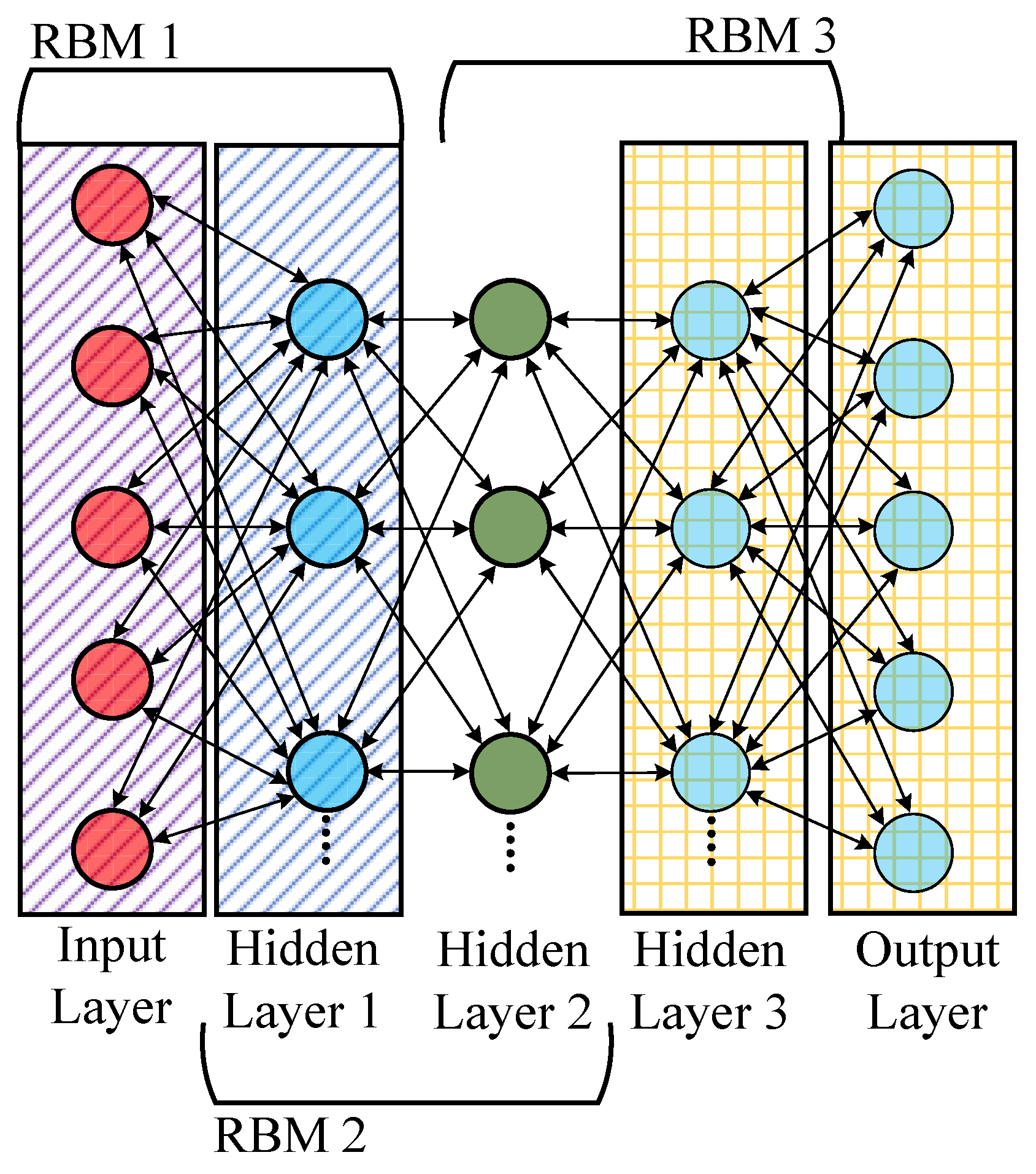
Figure 1 illustrates the DBN training process. The vector v denotes the state of the visible layer, while b represents its corresponding bias. Similarly, h refers to the hidden layer (HL) state vector, with c indicating the bias associated with the hidden layer.

4.2. Long Short-Term Memory (LSTM)

The LSTM-based forecasting model addresses several challenges effectively in power load estimation within distribution networks by modeling temporal dependencies, improving robustness against disturbances, and accommodating multi-dimensional input features.

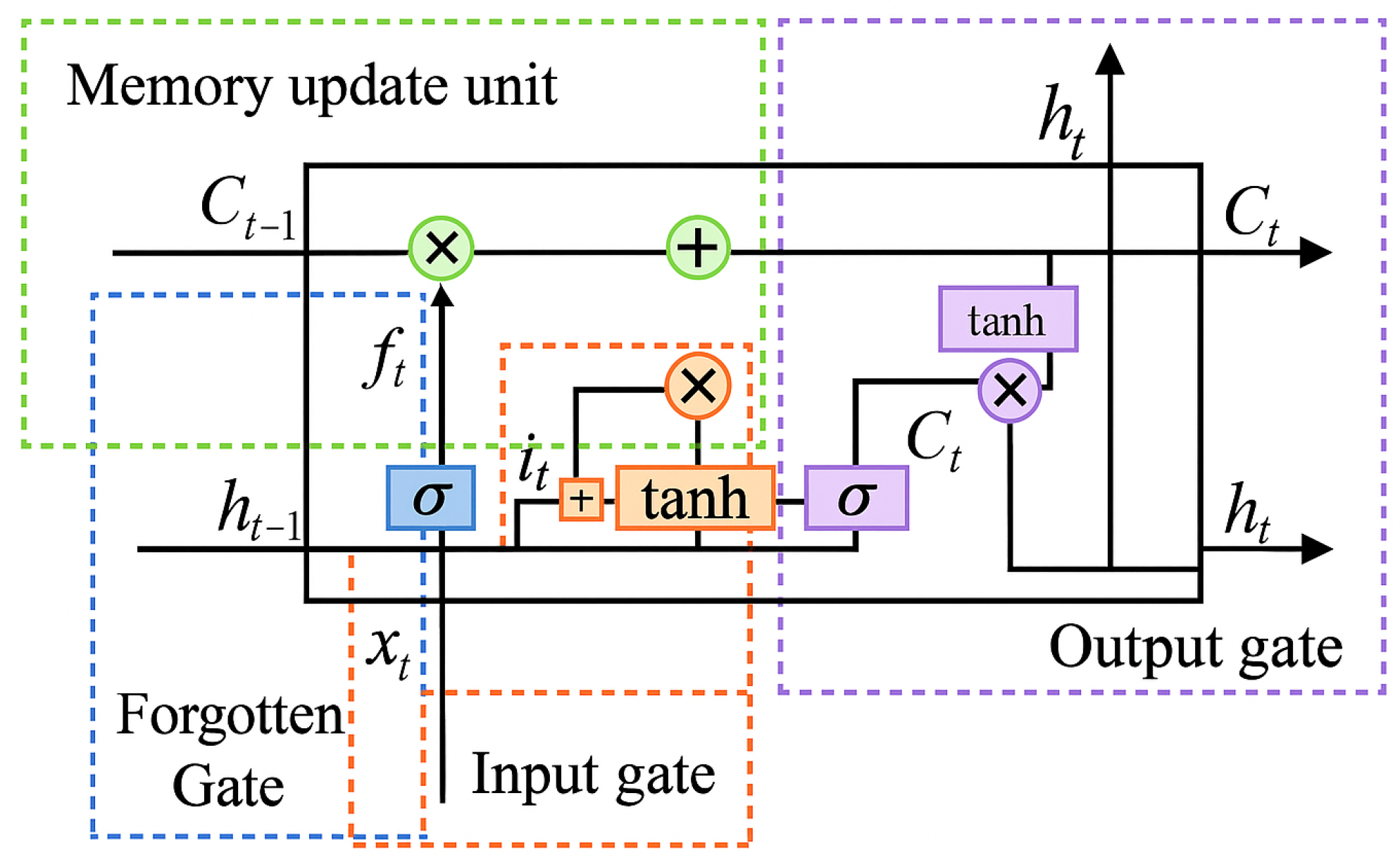
As illustrated in Figure 2, the Input Gate (IG), highlighted by the orange box, is the first component to be updated during the forward pass of the LSTM. It regulates the proportion of new information that flows into the memory cell. The output vector $o_{\mathrm{int}}$ of the IG and the candidate memory content $\tilde{C}\left(t\right)$ at time t are defined as follows:

$$\left\{\begin{array}{c}o\_i{n}_t=\sigma \left(W_{ix}·x_t+W_{ih}·h_{t-1}+b_i\right)\hfill \\ \tilde{C}\left(t\right)=o\_i{n}_t·\tanh \left(W_{zx}·x_t+W_{zh}·h_{t-1}+b_z\right)\hfill \end{array}\right.$$

(31)

where $h_{t-1}$ denotes the previous hidden state processed by the Sigmoid function $\sigma (·)$, and $x_t$ represents the current input processed by the Tanh function $\tanh (·)$. $W_{ix}$, $W_{ih}$, $W_{zx}$, and $W_{zh}$ are the corresponding weight matrices, while $b_i$ and $b_z$ are the bias terms for the input gate and candidate state, respectively. The forget gate, highlighted in the blue box, determines which information from the previous memory cell should be retained. Its output $o_{ft}$ at time t is given as follows:

$$o_{-}{f}_t=\sigma \left(W_{fx}·x_t+W_{fh}·h_{t-1}+b_f\right)$$

(32)

where $W_{fx}$ and $W_{fh}$ are weight matrices, and $b_f$ is the bias vector of the forget gate. As shown in the green box of Figure 2, the memory unit is updated by combining the dot product of $o_{ft}$ and $\tilde{C}\left(t\right)$ with the input gate output, resulting in the updated memory state $C_t$. The output gate, highlighted in purple, operates similarly to the input gate, defined as follows:

$$\left\{\begin{array}{c}{o}_t=\sigma \left(W_{ox}·x_t+W_{oh}·h_{t-1}+b_o\right)\hfill \\ h_t=o_t·\tanh \left(C_t\right)\hfill \end{array}\right.$$

(33)

where $W_{ox}$ and $W_{oh}$ denote the weight matrices and $b_o$ represents the bias vector. These parameters are updated during training via backpropagation through time (BPTT). Model training involves error analysis with two types of backpropagation: temporal and layer-wise. Temporal backpropagation propagates the error to any time step k, resulting in the error term ${\delta }_k^T$, as follows:

$${\delta }_k^T={\mathrm{\Pi }}_{j=k}^{t-1}{\delta }_{o,j}^{\mathrm{T}}{W}_{oh}+{\delta }_{f,j}^{\mathrm{T}}{W}_{fh}+{\delta }_{i,j}^{\mathrm{T}}{W}_{ih}+{\delta }_{c,j}^{\mathrm{T}}{W}_{ch}$$

(34)

where ${\delta }_{o,j}^{\mathrm{T}}$, ${\delta }_{f,j}^{\mathrm{T}}$, ${\delta }_{i,j}^{\mathrm{T}}$, and ${\delta }_{c,j}^{\mathrm{T}}$ represent the error terms for the output gate, forget gate, input gate, and memory unit, respectively. To propagate the error to the next layer, the error term ${\delta }_t^{l-1}$ and the input $x_t^l$ of layer l are computed based on the output of layer $l-1$ at time t, as follows:

$$\left\{\begin{array}{c}{\delta }_t^{l-1}={\displaystyle \frac{\partial E}{{\mathrm{net}}_t^{l-1}}}\hfill \\ x_t^l=f^{l-1}\left({\mathrm{net}}_t^{l-1}\right)\hfill \end{array}\right.$$

(35)

where $f^{l-1}$ signifies the activation function of layer $l-1.{\displaystyle \frac{\partial E}{{\mathrm{net}}_t^{l-1}}}$ represents the upward propagation of errors, as follows:

$${\displaystyle \frac{\partial E}{{\mathrm{net}}_t^{l-1}}}=\left({\delta }_{f,t}^l{W}_{fx}+{\delta }_{i,t}^l{W}_{ix}+{\delta }_{c,t}^l{W}_{cx}+{\delta }_{o,t}^l{W}_{ox}\right)·f^{\prime }\left({\mathrm{net}}_t^{l-1}\right)$$

(36)

The forward propagation process of LSTM involves a total of eight weight gradients. The four weight gradients ${\displaystyle \frac{\partial E}{\partial W_{oh,t}}},{\displaystyle \frac{\partial E}{\partial W_{fh,t}}},{\displaystyle \frac{\partial E}{\partial W_{ih,t}}}$, and ${\displaystyle \frac{\partial E}{\partial W_{ch,t}}}$ for storing information updates in the memory unit at time t are calculated as follows:

$$\left\{\begin{array}{c}{\displaystyle \frac{\partial E}{\partial W_{oh,t}}}={\displaystyle \frac{\partial E}{\partial o_{-}{o}_t}}·{\displaystyle \frac{\partial o_{-}{o}_t}{\partial W_{oh,t}}}={\delta }_{o,t}{h}_{t-1}^T\hfill \\ {\displaystyle \frac{\partial E}{\partial W_{fh,t}}}={\displaystyle \frac{\partial E}{\partial o_{-}{f}_t}}·{\displaystyle \frac{\partial o_{-}{f}_t}{\partial W_{fh,t}}}={\delta }_{f,t}{h}_{t-1}^T\hfill \\ {\displaystyle \frac{\partial E}{\partial W_{ih,t}}}={\displaystyle \frac{\partial E}{\partial o_{-}i{n}_t}}·{\displaystyle \frac{\partial o_{-}i{n}_t}{\partial W_{ih,t}}}={\delta }_{i,t}{h}_{t-1}^T\hfill \\ {\displaystyle \frac{\partial E}{\partial W_{ch,t}}}={\displaystyle \frac{\partial E}{\partial c_t}}·{\displaystyle \frac{\partial c_t}{\partial W_{ch,t}}}={\delta }_{c,t}{h}_{t-1}^T\hfill \end{array}\right.$$

(37)

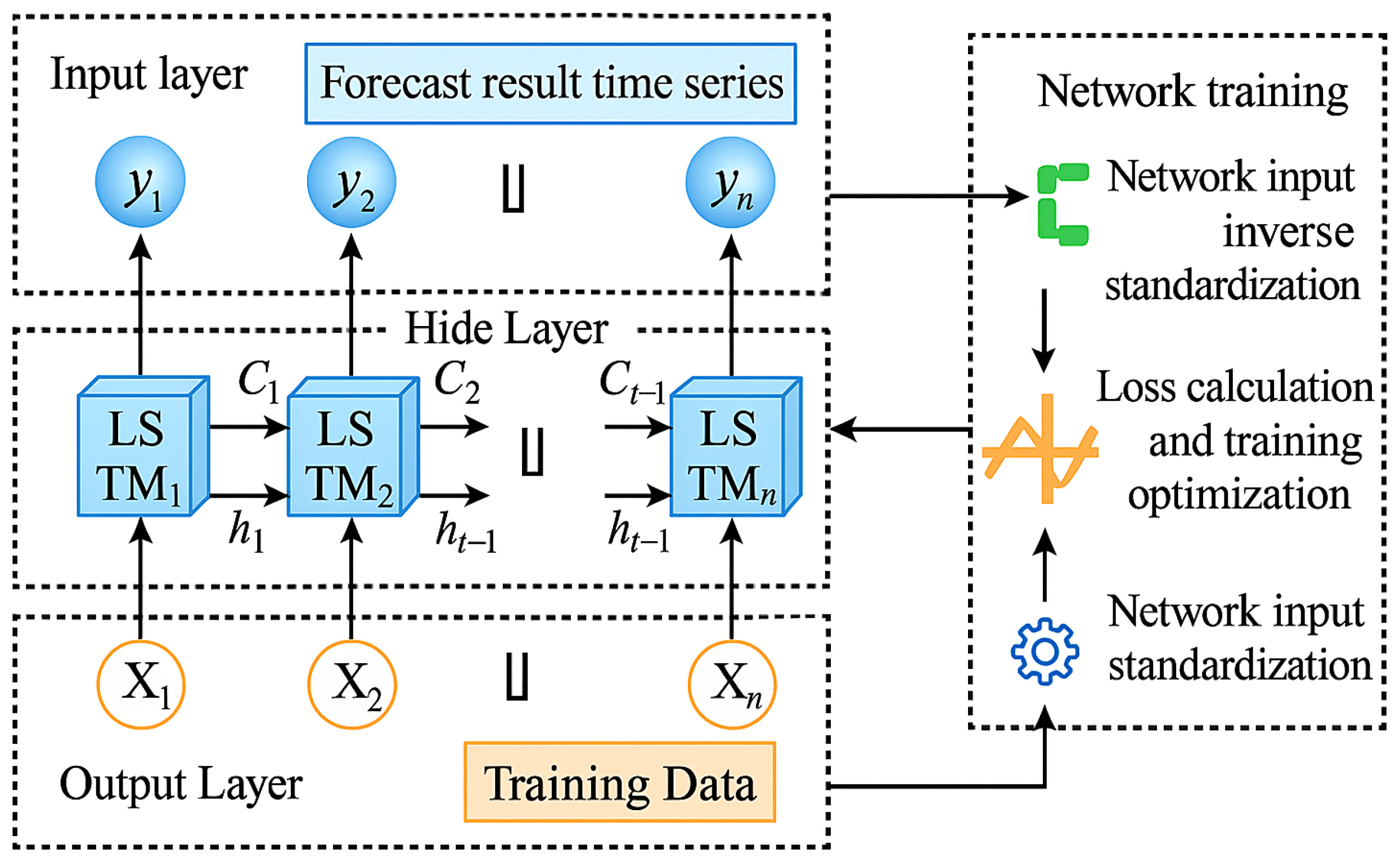
Weight gradients are computed at each time step and summed to obtain the final gradient in Equation (37). The gradients of $W_{fx}$, $W_{ix}$, $W_{cx}$, and $W_{ox}$ are calculated similarly based on their respective error terms. However, for power load forecasting, the LSTM architecture requires further optimization. The structure of the LSTM-based prediction model is illustrated in Figure 3.

As shown in Figure 3, the input layer uses frequency domain and statistical characteristics from actual power load data. Training data are normalized via min–max scaling for faster convergence, and predictions are recovered through inverse normalization after model training and validation.

$$x={\displaystyle \frac{x^{\prime }\left(x_{\max }-x_{\min }\right)+\left(x_{\max }+x_{\min }\right)}{2}}$$

(38)

According to Equation (38), the predicted results are denormalized to match the original power load data in units and scale, making them easier to interpret. This allows for direct comparison with actual data and enables performance evaluation through error and accuracy metrics.

4.3. DBN-LSTM

There are m visible neurons and n hidden neurons in the RBM. The essence of the RBM is an Energy-Based Model (EBM). For a set of given states, this state energy is presented as follows:

$$E(v,h\mid \theta )=-\sum _{i=1}^m{b}_i{v}_i-\sum _{j=1}^n{c}_j{h}_j-\sum _{i=1}^m\sum _{j=1}^n{v}_i{w}_{ij}{h}_j$$

(39)

where $(v,h)$ represents a predefined state. In the context of power load forecasting, the energy function characterizes the interaction between the visible and hidden layers, guiding the network’s learning objective. Minimizing this function enables the model to extract more informative features from the input data, thereby enhancing its forecasting accuracy.

$$E(v,h)=-b^{\mathrm{T}}v-c^{\mathrm{T}}h-h^{\mathrm{T}}Wv$$

(40)

The RBM connects the visible and hidden layers through the weight matrix W. The energy function $E(v,h|\theta )$ quantifies their interaction. In load forecasting, this enables the model to assess how visible–hidden relationships influence predictions. Given parameters $\theta$, the joint probability distribution is defined in (41).

$$\left\{\begin{array}{c}p(v,h\mid \theta )={\displaystyle \frac{e^{-E(v,h\mid \theta )}}{Z\left(\theta \right)}}\hfill \\ Z\left(\theta \right)=\sum _{v,h}{e}^{-E(v,h)}\hfill \end{array}\right.$$

(41)

In (41), p is the joint probability and $Z\left(\theta \right)$ is the partition function. Marginalizing hidden states yields the visible distribution. Given v, the activation of the hidden neurons is calculated by (42).

$$p\left(h_j=1\mid v\right)=\mathrm{sigmoid}\left(c_j+\sum _i{v}_i{w}_{ij}\right)$$

(42)

If the HL state vector h is presented, the activation probability of neurons in the visible layer is displayed as follows:

$$p\left(v_j=1\mid h\right)=\mathrm{sigmoid}\left(b_j+\sum _i{h}_i{w}_{ij}\right)$$

(43)

Equations (42) and (43) utilize the sigmoid function to activate the visible layer based on hidden features, enabling short-term load prediction. The key lies in modeling the probability distribution of the visible layer v, with its marginal form shown in (44).

$$p\left(v\right)={\displaystyle \frac{1}{Z\left(\theta \right)}}\sum _h{e}^{-E(v,h\mid \theta )}$$

(44)

where $p\left(v\right)$ signifies the edge distribution of the visible layer. The edge distribution of HL h is obtained, as displayed as follows.

$$p\left(h\right)={\displaystyle \frac{1}{Z\left(\theta \right)}}\sum _v{e}^{-E(v,h\mid \theta )}$$

(45)

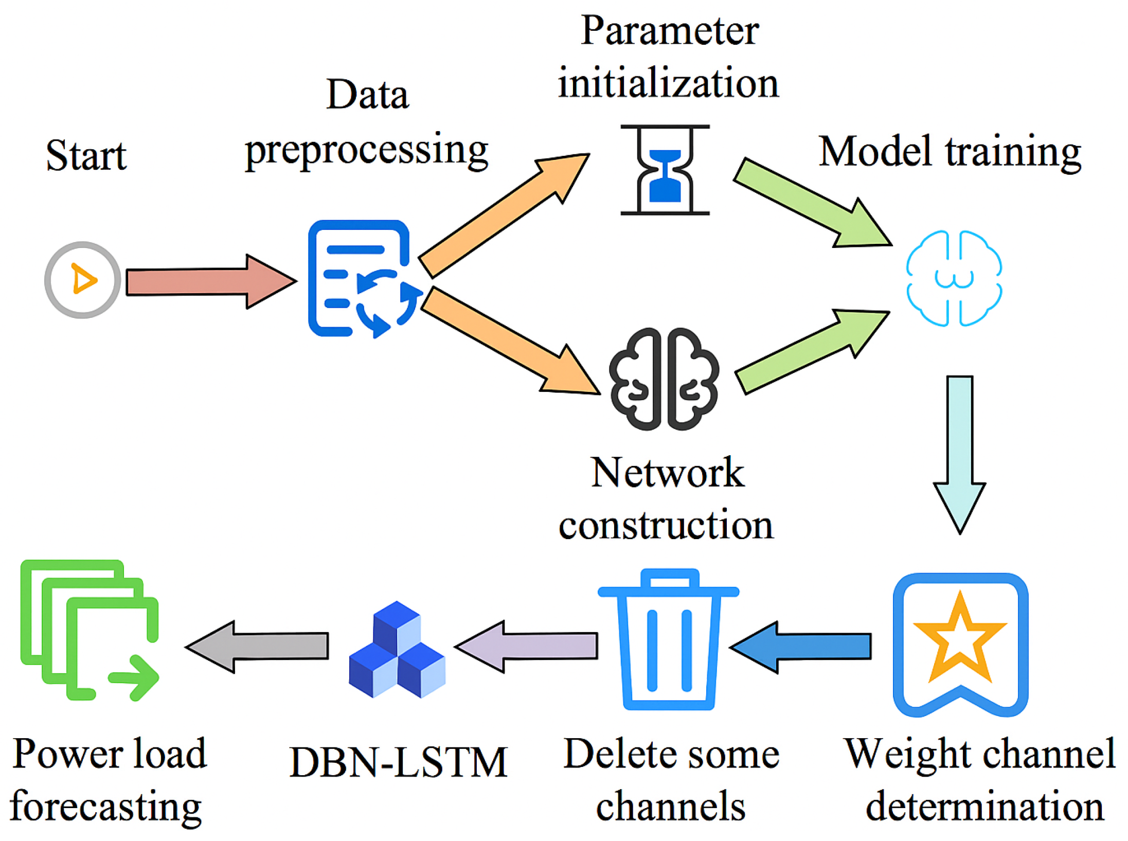
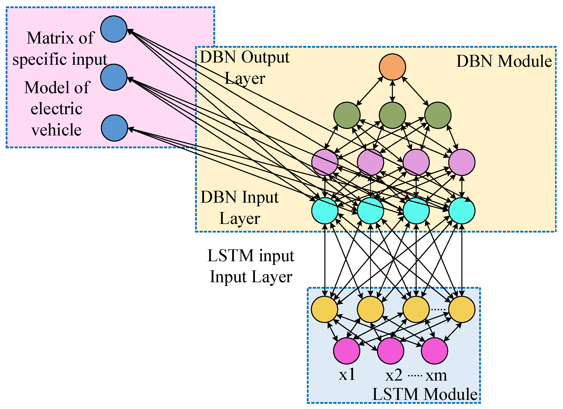
To align the model’s probability distribution with that of the training data, RBM training involves optimizing the parameter set $\theta$. Building upon this concept, the power load forecasting framework is introduced, leveraging the DBN-LSTM architecture as its foundation, as depicted in Figure 4.

Power load data are first processed by a DBN for feature extraction and dimensionality reduction, then fed into an LSTM to capture temporal dependencies. This DBN–LSTM cascade enhances the model’s ability to represent dynamic load patterns through deep feature abstraction. When combined with LSTM, the learning capability and prediction accuracy can be further enhanced. The DBN inherently consists of an unsupervised RBM, as illustrated in Figure 5.

5. Optimization-Based Load Shedding Strategy Under Stability Constraints

In high-renewable power systems, frequency recovery after disturbances may still leave the network vulnerable to voltage instability. To address this, a stability-constrained optimal load-shedding strategy is proposed, employing discrete group search optimization to restore frequency while maximizing voltage stability margins. Load uncertainty, the primary stochastic factor, is incorporated via point estimation to ensure robust stability under variable operating conditions.

5.1. An Adaptive Load Shedding Methodology

Load shedding can be formulated as a discrete optimization problem requiring efficient solution methods. This work employs a Discrete Group Search Optimizer (DGSO), an extension of the Binary GSO, to determine optimal actions under steady-state constraints. A probabilistic centralized adaptive scheme is developed in this paper to enhance voltage stability margins, thereby reducing collapse risk after major disturbances.

The load shedding problem is formulated as a discrete probabilistic optimization problem, where the objective is to maximize the expected voltage stability margin of the system in per-unit (p.u.). Let $\mathbf{u}=\left[u_1,u_2,\dots ,u_m\right]$ denote the load shedding decision vector, in which each $u_j$ represents the load feeder to be shed at bus j and takes discrete values. The optimization model is expressed as

$$\begin{array}{cc}\hfill \underset{\mathbf{u}}{\max }& \mathbb{E}\left[\mathrm{PV}\_\mathrm{Margin}(\mathbf{x},\mathbf{u})\right]\hfill \\ \hfill \mathrm{s}.\mathrm{t}.& \mathbf{x}=f(\mathbf{x},\mathbf{u},\mathbf{d})\hfill \\ \hfill & V_i^{\min }\le V_i\left(\mathbf{x}\right)\le V_i^{\max },\forall i\hfill \\ \hfill & 0\le u_j\le u_j^{\max },\forall j\hfill \end{array}$$

(46)

where $\mathrm{PV}\_\mathrm{Margin}(\mathbf{x},\mathbf{u})$ denotes the voltage stability margin of the system corresponding to the load shedding action $\mathbf{u}$. The operator $E\left[·\right]$ represents the expected value, considering the probabilistic nature of large disturbances $\mathbf{d}$. The state vector $\mathbf{x}$ is determined by the system’s nonlinear power flow equations under the selected shedding scheme. The load feeders are treated as discrete optimization variables, and in this work, the DGSO algorithm is employed to effectively explore the search space. In DGSO, each member of the population corresponds to a candidate load shedding vector $\mathbf{u}$, enabling efficient identification of the solution that maximizes the system’s expected voltage stability margin.

5.2. Probabilistic Discrete Group Search Optimization Method

GSO is a population-based heuristic algorithm in which individuals (members) form a group and assume one of three roles: producer (best-positioned member with vision), scrounger (follows the producer), or ranger (random exploration).

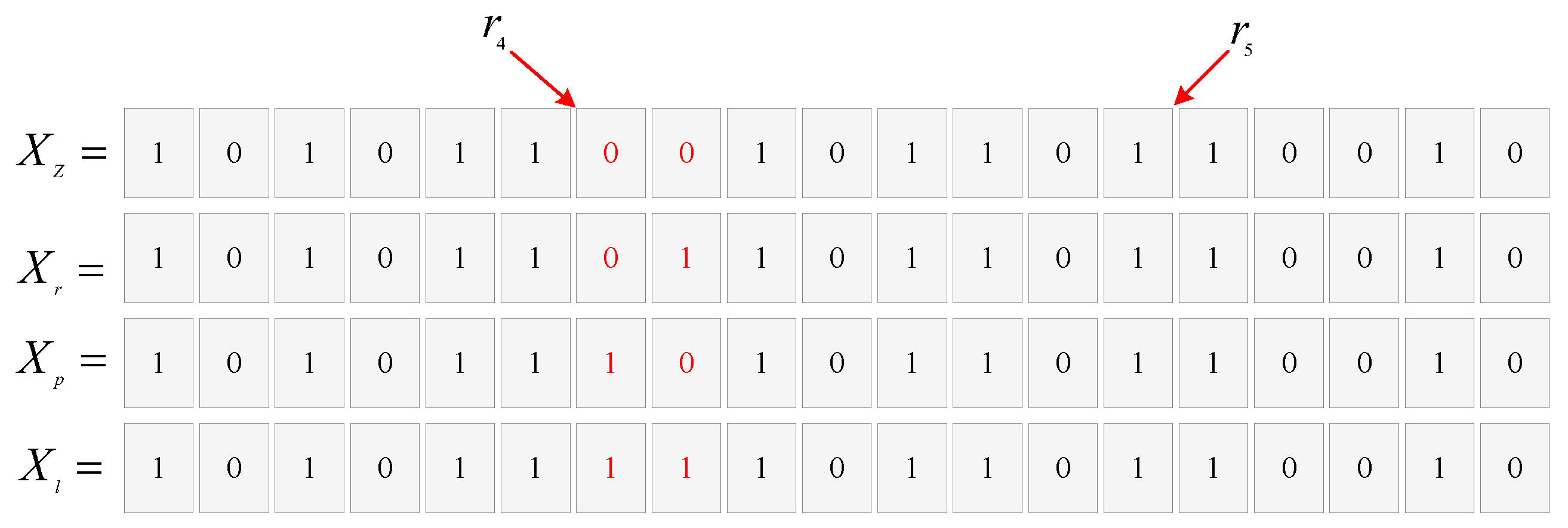
Within the GSO method, three reference positions are selected, referred to as zero, right, and left. During the ${\kappa }^{\mathrm{th}}$ iteration, for the producer individual situated at $X_p^{\kappa }$, the zero, right, and left positions are determined according to Equations (47)–(49), respectively.

$$X_z=X_p^{\kappa }+r_1{l}_{\max }{D}_p^{\kappa }\left({\phi }^{\kappa }\right)$$

(47)

$$X_r=X_p^{\kappa }+r_1{l}_{\max }{D}_p^{\kappa }\left({\phi }^{\kappa }+r_2{\theta }_{\max }/2\right)$$

(48)

$$X_l=X_p^{\kappa }+r_1{l}_{\max }{D}_p^{\kappa }\left({\phi }^{\kappa }-r_2{\theta }_{\max }/2\right)$$

(49)

where $r_1$ and $r_2$ represent random variables following normal and uniform distributions, respectively, with zero mean and a standard deviation of 1. The parameters $l_{max}$ and $h_{max}$ denote the maximum pursuit distance and maximum pursuit angle, respectively. Their values can be computed as follows:

$$l_{\max }=\parallel U-L\parallel =\sqrt{\sum _{i=1}^n{\left(U_i-L_i\right)}^2}$$

(50)

$${\theta }_{\max }={\displaystyle \frac{\pi }{a^2}}$$

(51)

where $U_i$ and $L_i$ denote the upper and lower bounds of the i-th variable, respectively, while n represents the dimensionality of the search space. The parameter a in Equation (52) is determined as follows:

$$a=round\left(\sqrt{n+1}\right)$$

(52)

where round indicates the rounding operator. In Equations (48)–(50), $D_i^{\kappa }\left({\phi }_i^{\kappa }\right)$ is the search direction vector of the i-th member at the ${\kappa }^{\mathrm{th}}$ iteration. Each member of the search direction vector, $d_{ij}^{\kappa }$, can be calculated as follows:

$$\begin{array}{cc}\hfill & D_i^{\kappa }\left({\phi }_i^{\kappa }\right)=\left(d_{i1}^{\kappa },\dots ,d_{in}^{\kappa }\right)\in {\Re }^n\hfill \\ \hfill & d_{ij}^{\kappa }=\left\{\begin{array}{cc}\prod _{q=1}^{n-1}\cos \left({\phi }_{iq}^{\kappa }\right)\hfill & j=1\hfill \\ \sin \left({\phi }_{i(j-1)}^{\kappa }\right)\prod _{q=j}^{n-1}\cos \left({\phi }_{iq}^{\kappa }\right)\hfill & j=2,\dots ,n-1\hfill \\ \sin \left({\phi }_{i(n-1)}^{\kappa }\right)\hfill & j=n\hfill \end{array}\right.\hfill \end{array}$$

(53)

5.3. Binary Search Space

In binary searching space, all the members of the GSO group are either 0 or 1. In Figure 6 random length selection for the producer member is illustrated. According to Figure 6, for $(1\times n)$ array, $r_4$ is a random pointer in the range of $(1,n)$ and $r_5$ is also a random pointer in the range $(r_4,n)$. In addition, the term $X_p^{\kappa }-X_i^{\kappa }$ can be formulated as follows:

$$X_p^{\kappa }-X_i^{\kappa }=XOR\left(X_p^{\kappa },X_i^{\kappa }\right)$$

(54)

where $X_p^{\kappa }$ is the producer member position at the $\kappa$-th iteration and $X_i^{\kappa }$ is the i-th scrounger member at the $\kappa$-th iteration. The $XOR$ function ($\Delta X_i^k$) is defined as follows:

$$XOR(a,b)=\left\{\begin{array}{cc}1\hfill & a\ne b\hfill \\ 0\hfill & a=b\hfill \end{array}\right.$$

(55)

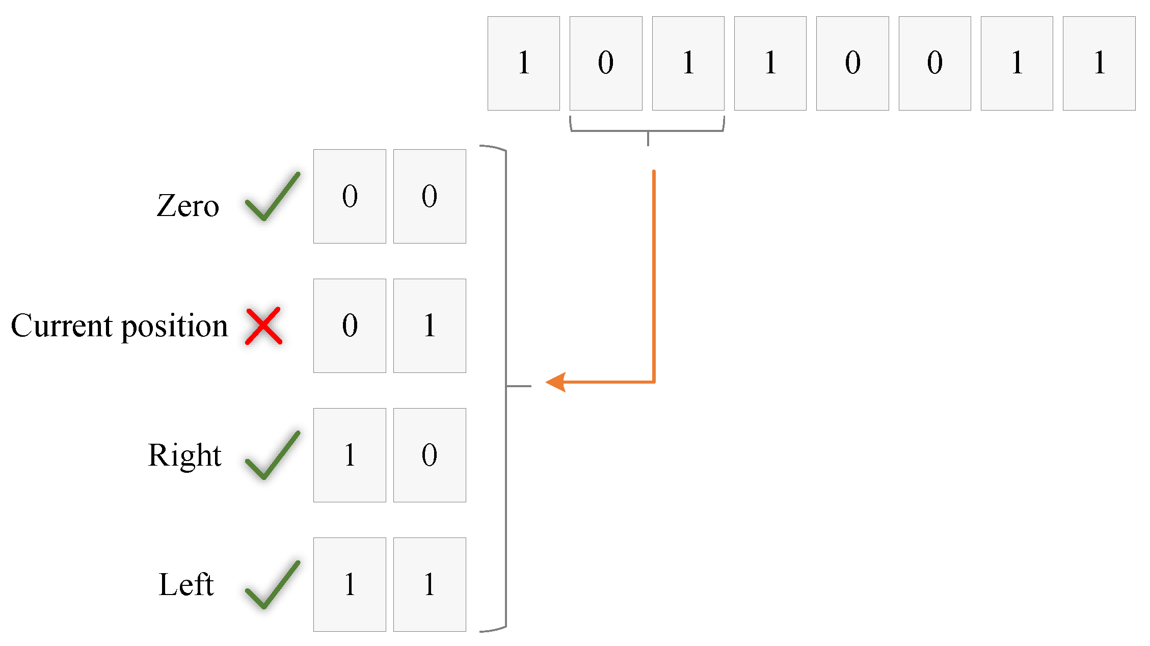
After calculating the term $X_p^{\kappa }-X_i^{\kappa }$, a random segment length is determined using the pointers $r_6$ and $r_7$. Figure 7 illustrates the simulation of the operation $r\circ \left(X_p^{\kappa }-X_i^{\kappa }\right)$. As shown in Figure 7, for a $(1\times n)$ array, $r_6$ is a randomly generated number within $(1,n)$, and $r_7$ is another random number chosen within $\left(r_6,n\right)$. The resulting sub-array consists of elements 0 and 1. The entries with value 1 indicate the positions where the producer and the i-th scrounger differ in that column. Consequently, the corresponding columns of the selected sub-array will undergo a state change.

5.4. Probabilistic DSGO for Load Shedding

In this section, a DGSO model is formulated for the load shedding problem. The method extends the binary GSO (BGSO) to a generalized discrete form. As shown in Figure 8, the constructed array A represents the discrete search space, projected from the binary search space. Each element $a_1,a_2,a_3,\dots$ corresponds to an n-dimensional candidate solution selected during DGSO execution. A DGSO member can occupy positions such as $a_1,a_2,a_3$, or their sums (e.g., $a_1+a_2$, $a_1+a_3$, $a_1+a_2+a_3$, etc.). The following subsections detail the DGSO components.

5.4.1. Producer

In the proposed DGSO, once the three binary arrays—zero ($X_z$), right ($X_r$), and left ($X_l$)—are generated, their corresponding representations in the discrete search space can be expressed using array A as follows:

$${\widehat{X}}_z=X_z·A^T$$

(56)

$${\widehat{X}}_r=X_r·A^T$$

(57)

$${\widehat{X}}_l=X_l·A^T$$

(58)

where ${\widehat{X}}_z$, ${\widehat{X}}_r$, ${\widehat{X}}_l$ represent the zero, right and left points in the discrete space.

As in BGSO, each pair of consecutive columns in the selected sub-array represents a stage of head-angle adjustment. Points from the first stage are evaluated before proceeding. In the second stage, the next consecutive pair in the binary array is chosen (Figure 9), and the DGSO production step is applied to the binary producer using Equations (56)–(58).

5.4.2. Scroungers

Once the binary-space scroungers have been selected, the scrounging behavior in DGSO can then be represented using the following:

$${\widehat{X}}_i^{\kappa }=X_i^{\kappa }·A^T$$

(59)

where $X_i^{\kappa }$ and ${\widehat{X}}_i^{\kappa }$ represent the i-th scrounger location at the $\kappa \mathrm{th}$ iteration in the binary and discrete spaces, respectively.

5.4.3. Rangers

In BGSO, the ranging process is carried out by defining a random length, while the random direction is determined according to the procedure described in Section 5.3. The binary-space ranger member, denoted by $X_i^j$, is then generated. Subsequently, the DGSO ranger member can be formulated as follows:

$${\widehat{X}}_i^j=X_i^j·A^T$$

(60)

5.5. Point Estimate Method

Due to the inherent uncertainty in future power system conditions—primarily load variability—probabilistic analysis is crucial for reliable load shedding. This paper adopts the Point Estimation Method (PEM) to model load uncertainty, efficiently approximating probabilistic problems with minimal iterations using only key statistics (variance, skewness, kurtosis) instead of full distributions.

PEM evaluates the objective function at a set of deterministically chosen points, ensuring convergence with low computational cost. The main PEM steps are as follows: for each random variable, k points are determined to compute the PV margin and fitness function.

$$\left({\mu }_{p1},{\mu }_{p2},\dots ,P_{l,k},\dots ,{\mu }_{pm}\right)$$

(61)

where ${\mu }_{pl}$ stands for the mean value of the l-th input variable. Additionally, $P_{l,k}$, the k-th point of the l-th input variable, is defined as follows:

$$P_{l,k}={\mu }_{pl}+{\xi }_{l,k}{\sigma }_{pl}$$

(62)

where ${\sigma }_{pl}$ is the standard deviation of the l-th input random variable. The ${\xi }_{l,k}$ is the standard location which would be calculated according to the total number of estimated points. For instance, for $2m+1$ PEM, standard locations can be calculated implementing Equations (63)–(65).

$${\xi }_{l,1}={\displaystyle \frac{{\lambda }_{l,3}}{2}}+\sqrt{{\lambda }_{l,4}-{\displaystyle \frac{3}{4}}{\lambda }_{l,3}^2}$$

(63)

$${\xi }_{l,2}={\displaystyle \frac{{\lambda }_{l,3}}{2}}-\sqrt{{\lambda }_{l,4}-{\displaystyle \frac{3}{4}}{\lambda }_{l,3}^2}$$

(64)

$${\xi }_{l,3}=0$$

(65)

where ${\lambda }_{l,3}$ and ${\lambda }_{l,4}$ are the skewness and kurtosis of the l-th input variable. Afterwards, the sample points should be estimated and the fitness function for all estimated points should be evaluated. Finally, expected values of outputs will be calculated as final results:

$$E\left[Z\right]=\sum _{l=1}^m\sum _{k=1}^K{\omega }_{l,k}Z(l,k)$$

(66)

where Z is the vector of output random variables, $E\left[Z\right]$ is the expected value of vector Z and K is the total number of points; $2m+1$ PEM is used in the load shedding problem. ${\omega }_{l,k}$ is the weighting coefficient, which could be calculated for $2m+1$ PEM as follows:

$${\omega }_{l,k}={\displaystyle \frac{{(-1)}^{3-k}}{{\xi }_{l,k}\left({\xi }_{l,1}-{\xi }_{l,2}\right)}}k=1,2$$

(67)

$${\omega }_{l,3}={\displaystyle \frac{1}{m}}-{\displaystyle \frac{1}{{\lambda }_{l,4}-{\lambda }_{l,3}^2}}$$

(68)

where m is the number of input random variables.

5.6. Application of Probabilistic DGSO to the Load Shedding Problem

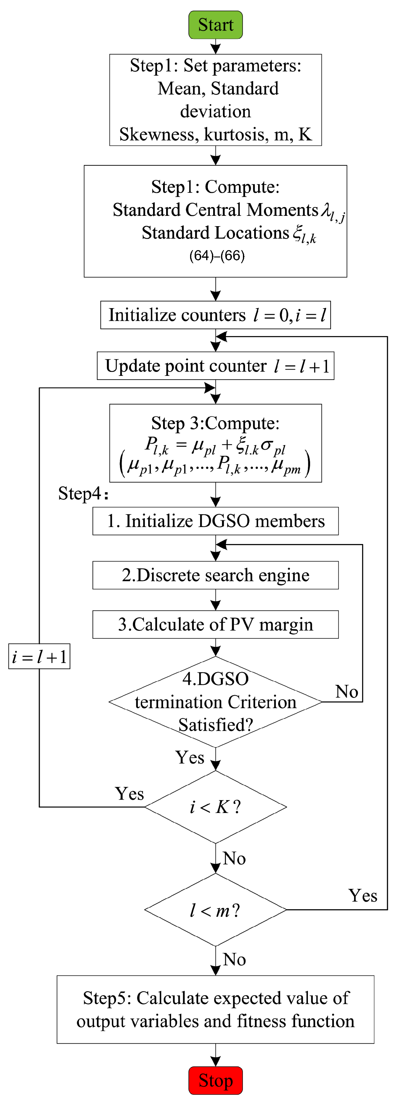
In the proposed method, DGSO members represent stochastic optimization variables, with potential load feeders defining the search space. Load uncertainty is modeled via the Point Estimation Method (PEM) (Figure 10).

Step 1: Define PEM inputs, including the number of estimation points K, random variables m, and load statistics (mean, standard deviation, skewness, kurtosis). For the shedding problem, the total load is the uncertain variable ($m=1$), and the $2m+1$ PEM scheme is applied (Equations (59)–(65)), yielding $K=3$ estimation points.

Step 2: Calculate standardized central moments ${\lambda }_{l,j}$ and locations ${\xi }_{l,k}$ (Equations (61)–(65)).

Step 3: Compute the DGSO input vector per Equation (59).

Step 4: Apply DGSO to select loads to shed, following these steps:

• Initialization: Load feeders serve as decision variables, with binary arrays encoding candidate loads forming the DGSO population (size fixed at 25). Initial members are generated randomly based on feeder counts.
• Discrete Search: DGSO evolves the population, with 40% scroungers and 60% rangers as per the simulation.
• Evaluation: PV margin and fitness function (Equation (46)) are used to assess each solution.
• Termination: The search stops upon reaching maximum iterations; otherwise, it loops back to Step 2. The PEM loop ends after all estimation points are processed; otherwise, it proceeds to Step 3.

Step 5: Final outputs and fitness are computed using weighting coefficients (Equations (66)–(68)).

6. Simulation and Experimental Study

6.1. Static Voltage Stability in High-Penetration Renewable Energy Systems

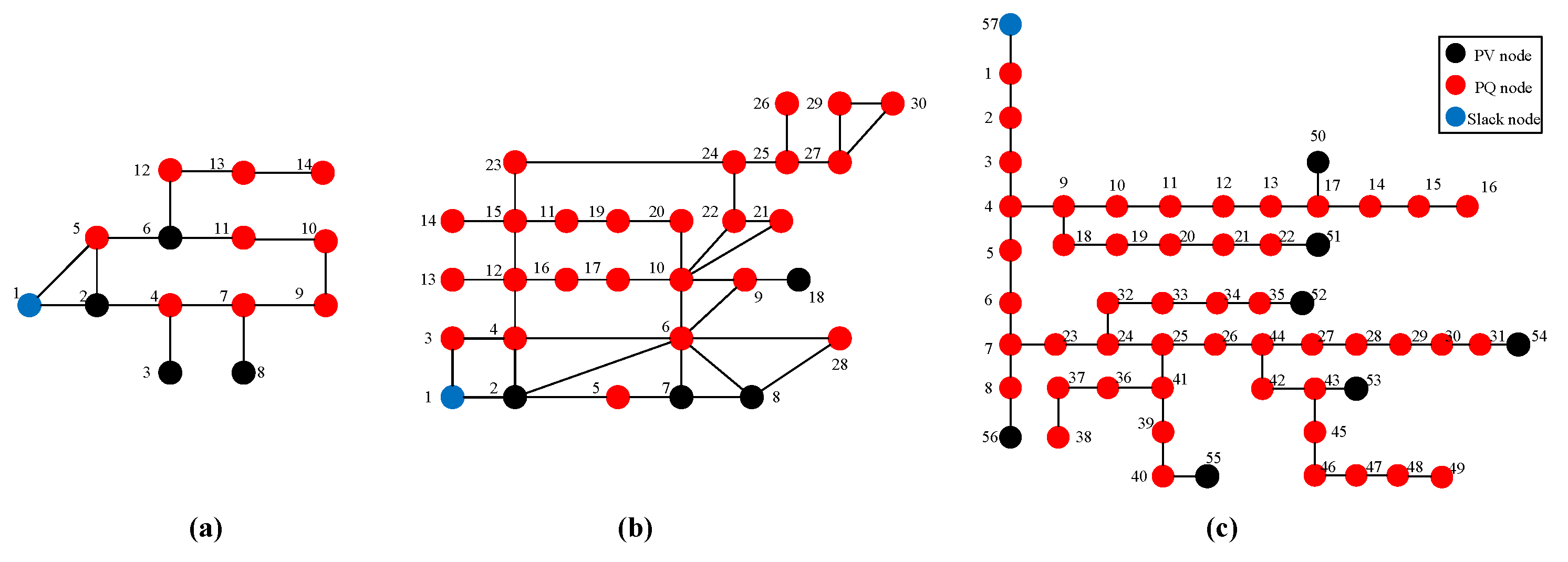
To verify the effectiveness and feasibility of the proposed method, the IEEE 14-bus, IEEE 30-bus, and IEEE 57-bus standard test systems are employed for simulation analysis, and their topological structures are shown in Figure 11. These systems are widely used in voltage stability studies and can effectively evaluate algorithm performance under different system scales and operating conditions.

In the simulations, the IEEE 30-bus system is selected as the primary test platform to conduct detailed analyses of stability region estimation, voltage boundary assessment, and algorithm iterations. The parameters of the IEEE 30-bus test system are listed in

Table A1. Line parameters of the IEEE 30-bus system.

Node1	Node2	R	X	Node1	Node2	R	X
1	2	0.019	0.058	15	11	0.107	0.219
1	3	0.045	0.165	11	19	0.064	0.129
2	4	0.057	0.174	19	20	0.034	0.068
3	4	0.013	0.038	10	20	0.094	0.209
2	5	0.047	0.198	10	17	0.032	0.085
2	6	0.058	0.176	10	21	0.035	0.075
4	6	0.012	0.041	10	22	0.073	0.150
5	7	0.046	0.116	21	22	0.012	0.024
6	7	0.027	0.082	15	23	0.100	0.202
6	8	0.012	0.042	22	24	0.115	0.179
6	9	0	0.208	23	24	0.132	0.270
6	10	0	0.556	24	25	0.189	0.329
9	18	0	0.208	25	26	0.254	0.380
9	10	0	0.110	25	27	0.109	0.209
4	12	0	0.256	28	27	0	0.396
12	13	0	0.140	27	29	0.220	0.415
12	14	0.123	0.256	27	30	0.320	0.603
12	15	0.066	0.130	29	30	0.240	0.453
12	16	0.094	0.199	8	28	0.063	0.200
14	15	0.221	0.200	6	28	0.017	0.060
16	17	0.052	0.192

and

Table A2. Node parameters of the IEEE 30-bus system.

Index	Type	V (pu)	${\mathit{P}}_{\mathit{g}}$ (pu)	${\mathit{Q}}_{\mathit{g}}$ (pu)	${\mathit{P}}_{\mathit{l}}$ (pu)	${\mathit{Q}}_{\mathit{l}}$ (pu)
1	1	1.05	–	–	0	0
2	2	1.045	0.576	0.024	0.217	0.127
3	3	–	–	–	0.024	0.012
4	3	–	–	–	0.076	0.016
5	3	–	–	–	0.228	0.109
6	3	–	–	–	0	0
7	2	1.05	0.179	0.176	0	0
8	2	1.01	0.35	0.323	0.3	0.3
9	3	–	–	–	0	0
10	3	–	–	–	0.058	0.02
11	3	–	–	–	0.032	0.009
12	3	–	–	–	0.112	0.075
13	3	–	–	–	0	0
14	3	–	–	–	0.062	0.016
15	3	–	–	–	0.082	0.025
16	3	–	–	–	0.035	0.018
17	3	–	–	–	0.09	0.058
18	2	1.05	0.169	0.250	0	0
19	3	–	–	–	0.095	0.034
20	3	–	–	–	0.022	0.007
21	3	–	–	–	0.175	0.112
22	3	–	–	–	0	0
23	3	–	–	–	0.032	0.016
24	3	–	–	–	0.087	0.067
25	3	–	–	–	0	0
26	3	–	–	–	0.035	0.023
27	3	–	–	–	0	0
28	3	–	–	–	0	0
29	3	–	–	–	0.024	0.009
30	3	–	–	–	0.106	0.019

in Appendix A. The IEEE 14-bus and IEEE 57-bus systems are further used for comparative validation.

6.1.1. Contour of Voltage Stability Limit Estimation

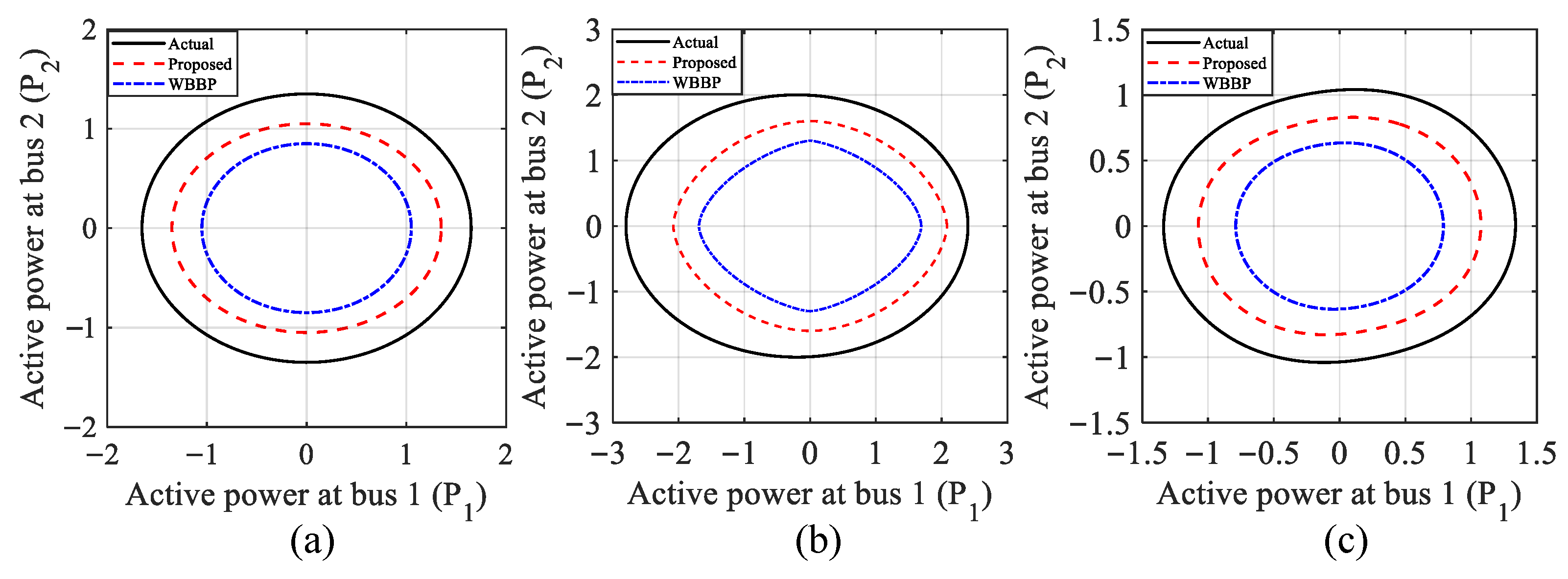
In the first case study, IEEE standard test systems are employed. For each test system, only the load directions of the first two designated load buses are varied. Their load magnitudes are set to be equal, and the 2-norm of their combined load power is made equivalent to the 2-norm of the remaining load buses. By sweeping the load directions of these two buses while maintaining a constant 2-norm for their power, the maximum global load scaling factors permitted by the condition proposed in this paper and by existing conditions are computed for each direction. These results are used to plot a two-dimensional contour of the voltage stability limit. The simulation results are presented in Figure 12. The solid black line represents the actual loadability boundary calculated via the continuation power flow method, the red dashed line corresponds to the condition proposed in this paper, and the blue dashed line represents the existing solvability condition.

Analysis of the simulation results leads to the conclusion that the proposed method yields the least conservative estimation of the voltage stability limit across all tested directions for every system. It demonstrates a significant improvement over the existing results.

6.1.2. Voltage Bound Estimation

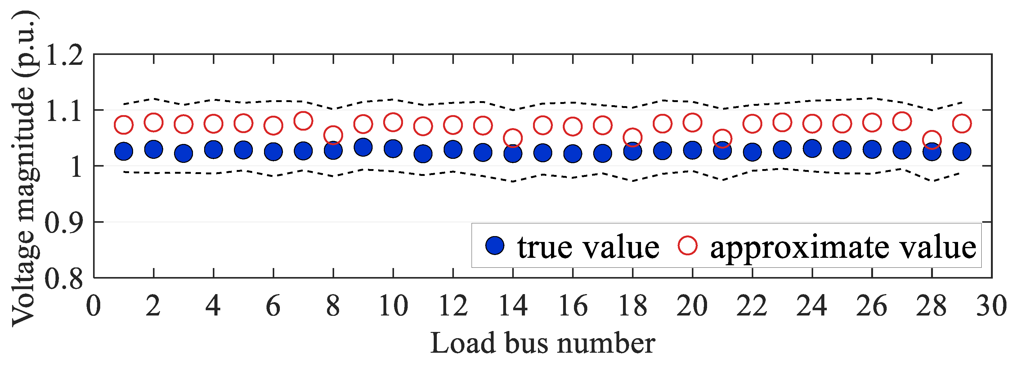
The primary objective of the second experiment is to evaluate the conservativeness and tightness of the voltage solution bounds (15) derived from Theorem 1. Tests are conducted on the IEEE 30-bus system under two scenarios: (i) the system operates at the base load condition; ($ii$) the system operates near the voltage stability limit, achieved by proportionally scaling up the total system load. For each load bus $i\in {\mathcal{N}}_L$, the upper and lower bounds for its voltage magnitude and phase angle are calculated according to Equation (15), where the parameter r is defined by Equation (22). Concurrently, the center point of $\overline{\mathcal{D}}\left(\underline{r}\right)$ (i.e., the voltage corresponding to $u_i=1-{\eta }_i$) is taken as the approximate estimate for that bus voltage. Upper and lower bounds for the voltage phase angle are obtained through a similar derivation.

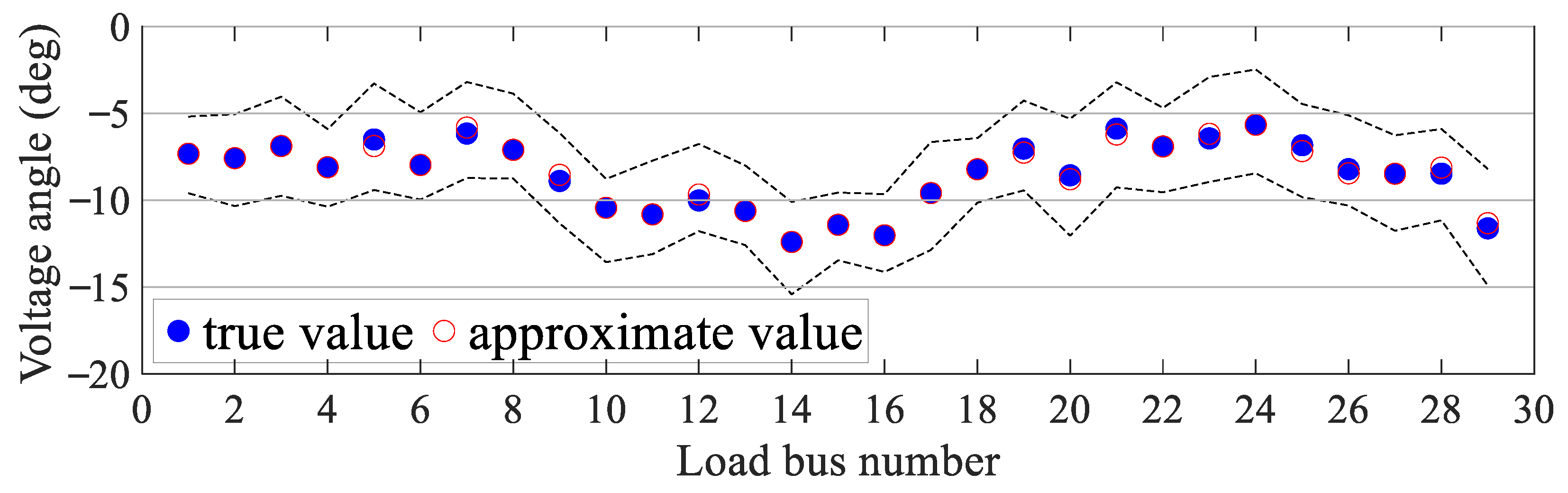
The actual voltage values (from power flow calculation), the approximate estimates, and the calculated bounds for all load buses are plotted in Figure 13 and Figure 14. In Figure 13, blue solid dots denote the actual voltage magnitudes at each bus, red hollow circles represent the approximate estimates provided by the proposed method, and the vertical dashed lines connecting the upper and lower bounds illustrate the computed voltage magnitude intervals. The results indicate that under the base load condition, all actual voltages lie in close proximity to their estimates and are contained within very narrow bounds. All magnitude estimation errors are below 0.1 p.u. Figure 14, using the same legend, displays the actual phase angles, their estimates, and the corresponding bounds. The results demonstrate that the method provides accurate quantitative estimates for both voltage magnitude and phase angle across all load buses, with magnitude errors less than 0.1 p.u. and phase angle errors less than 1 degree. This constitutes a significant reduction in conservativeness compared to traditional stability criteria.

6.1.3. The Iterative Process of the Algorithm

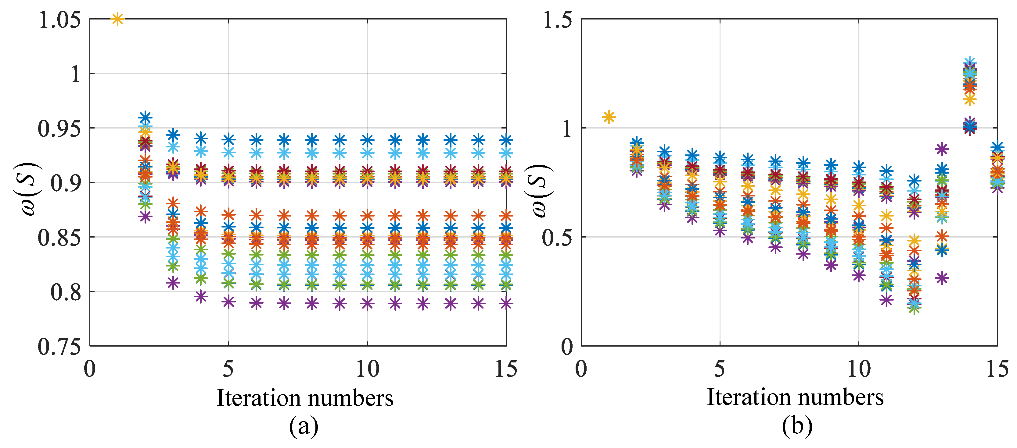
Let ${\parallel \varpi \left(\mathit{S}\right)\parallel }_{\infty }+{\parallel \varpi \left(\mathit{S}\right)\mathbf{1}\parallel }_{\infty }+2\sqrt{{\parallel \varpi \left(\mathit{S}\right)\mathbf{1}\parallel }_{\infty }{\parallel \varpi \left(\mathit{S}\right)\parallel }_{\infty }}=\tau$. According to Theorem 2, a unique steady-state voltage solution is guaranteed for the given power injections if $\tau <1$. Conversely, if $\tau \ge 1$, solution existence cannot be guaranteed. This criterion is examined through two scenarios with progressively increased load: In Case 1, within the per-unit system with the slack bus voltage $V_s$ as reference, $V_1=1.05\angle 0$, the system load is increased to 1.52 times the base value from Table 4 in reference [38]. The calculated value is $\tau =0.9759<1$, indicating that a steady-state solution should exist under this condition. In Case 2, the load is further increased to 2.4 times the base value, resulting in $\tau =1.5761>1$. The criterion suggests that no solution exists under this heavy load condition, implying operation beyond the voltage stability limit.

Figure 15 illustrates the iterative convergence of the solution algorithm for the two $\tau$ values. It clearly shows that the algorithm’s convergence strictly corresponds to the criterion $\tau <1$: the algorithm converges when the criterion is satisfied, confirming solution existence; it diverges when the criterion is not met.

6.2. Power Forecasting Based on the DBN–LSTM Model

6.2.1. Validation Method of the DBN–LSTM Model

(1)

Dataset Partition

The load data used in this study are obtained from the operational monitoring system of a municipal power grid. The dataset covers the period from 1 July 2025 to 1 August 2025, with a sampling interval of one minute. After data preprocessing and cleaning, a total of 18,800 valid samples were obtained. The dataset is divided into a training set and a test set with a ratio of 70% to 30%.

(2)

Overfitting Analysis

During the training process of deep learning models, the variation trends of training loss and validation loss can intuitively reflect the learning process and generalization capability of the model. Therefore, during the training stage of the DBN–LSTM model, the training loss and validation loss corresponding to each iteration are recorded simultaneously, and the model training status is analyzed by plotting the loss curves.

Training loss represents the value of the loss function calculated on the training dataset and is used to measure the model’s fitting ability to the training samples. In contrast, validation loss is calculated using the validation dataset and reflects the model’s predictive capability on unseen data. By comparing the variation trends of these two curves, it is possible to determine whether the model suffers from overfitting or underfitting.

(3)

Statistical Metrics

To comprehensively evaluate the prediction performance of the model, several statistical indicators are employed for quantitative analysis, including the Mean Absolute Error (MAE), Root Mean Square Error (RMSE), and Mean Absolute Percentage Error (MAPE). The corresponding formulas are defined as follows:

$$MAE={\displaystyle \frac{1}{N}}\sum _{i=1}^N|y_i-{\widehat{y}}_i|$$

(69)

$$RMSE=\sqrt{{\displaystyle \frac{1}{N}}\sum _{i=1}^N{(y_i-{\widehat{y}}_i)}^2}$$

(70)

$$MAPE={\displaystyle \frac{100\%}{N}}\sum _{i=1}^N\left|{\displaystyle \frac{y_i-{\widehat{y}}_i}{y_i}}\right|$$

(71)

where $y_i$ and ${\widehat{y}}_i$ denote the actual and predicted load values, respectively, and N is the number of samples. These metrics evaluate the prediction performance of the model from multiple perspectives.

6.2.2. Power Forecasting Design Based on the DBN–LSTM Model

(1)

Parameter Sensitivity Analysis of the DBN–LSTM Model

To determine the optimal parameter configuration of the DBN–LSTM model and further improve its prediction accuracy and stability in power load forecasting, a parameter sensitivity analysis is conducted using the control variable method. In this analysis, Mean Absolute Percentage Error (MAPE), Root Mean Square Error (RMSE), runtime (RT), and the retained weight ratio are adopted as the key evaluation metrics to identify the optimal parameter combination.

The sensitivity analysis focuses on three key parameters of the DBN–LSTM model, including the number of hidden layers, the number of neurons in the hidden layer, and the learning rate. The experimental results corresponding to different parameter settings are summarized in

Table 1. Parameter sensitivity analysis of the DBN–LSTM model.

Parameter Type	Parameter Value	MAPE (%)	RMSE (%)	RT (s)	Retained Weights (%)
Hidden layers	3	1.32	15.12	1.79	36
	4	1.16	13.23	1.97	35
	5	1.28	14.57	2.31	34
	6	1.69	17.83	2.75	33
Hidden neurons	15	1.93	19.27	1.65	37
	25	1.16	13.23	1.97	35
	35	1.21	13.89	2.14	34
	45	1.48	16.32	2.46	33
Learning rate	0.05	1.72	17.95	2.58	35
	0.1	1.16	13.23	1.97	35
	0.15	1.35	15.47	1.76	35
	0.2	1.89	19.62	1.63	35

.

As shown in Table 1, the optimal configuration for the number of hidden layers and neurons is four hidden layers with 25 neurons per layer. Under this configuration, the model achieves MAPE = 1.16%, RMSE = 13.23%, and RT = 1.97 s, representing an effective balance among feature extraction capability, model complexity, and computational efficiency. Deviations from this configuration, either in the number of hidden layers or the number of neurons, lead to overfitting or underfitting, resulting in a significant increase in MAPE.

For the pre-training stage, the optimal learning rate is found to be 0.1. A smaller learning rate prolongs the pre-training process, whereas an excessively large learning rate may cause gradient explosion and destabilize the training process.

(2)

Overfitting Analysis

During the training process of deep learning models, if the model performs well on the training dataset but exhibits a significant performance degradation on the test dataset, it indicates that the model may suffer from overfitting. Therefore, it is necessary to monitor and analyze the overfitting problem throughout the model training process.

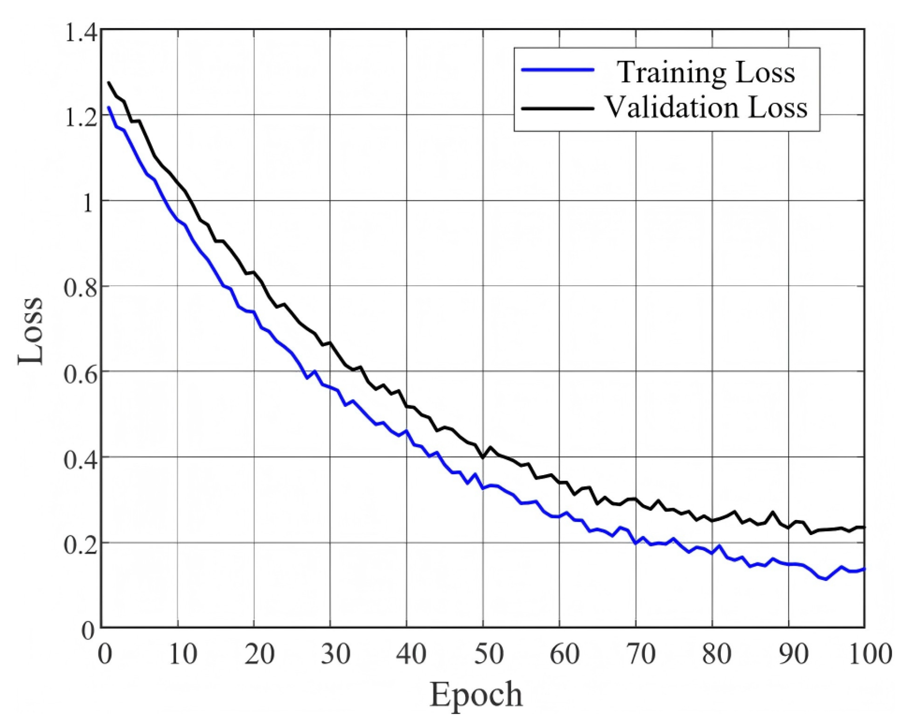
Figure 16 illustrates the variation trends of the training loss and validation loss of the DBN–LSTM model with respect to the number of training iterations (epochs). As shown in the figure, both the training loss and validation loss decrease rapidly during the early stages of training, indicating that the model is able to effectively learn the underlying features from the data. As the training process continues, the two curves gradually stabilize, suggesting that the model progressively converges.

6.2.3. Prediction Performance Evaluation of the DBN–LSTM Model

(1)

Comparison Between Predicted and Actual Values

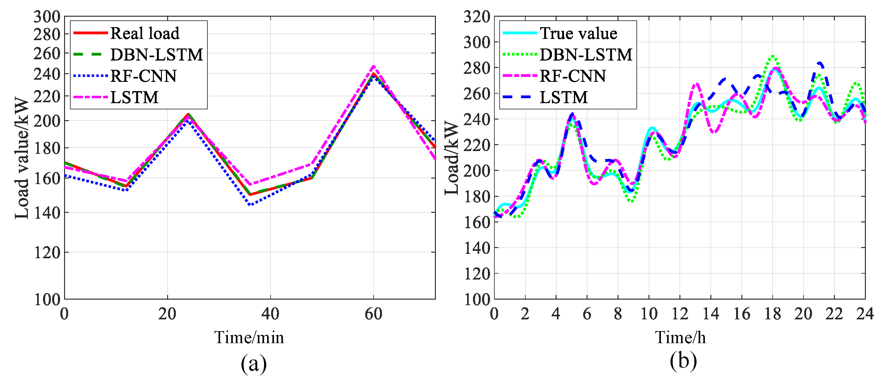
To evaluate the performance of the DBN–LSTM model in load forecasting, the predicted load values are compared with the actual load values, as shown in Figure 17. The figure also presents the prediction results obtained by the DBN–LSTM, RF–CNN, and LSTM models, allowing for a comprehensive comparison of the forecasting performance among different methods.

Figure 17a illustrates the comparison between the predicted and actual load values within a short time window. The selected time interval is extracted from the original load data sequence and represents a continuous segment that reflects the load variation characteristics over a short time scale, as well as the model’s capability to track load fluctuations. The results show that the DBN–LSTM model can accurately capture the trend of load variations, whereas the RF–CNN and LSTM models exhibit noticeable deviations at certain time points, particularly near the load peak periods.

Figure 17b presents the load forecasting results over a daily time scale. The system load exhibits a typical daily pattern, with higher values during daytime and evening periods and lower values at night. In comparison, the DBN–LSTM model demonstrates higher prediction accuracy near both peak and valley load periods. Overall, the results demonstrate the superior forecasting accuracy and trend-tracking capability of the proposed DBN–LSTM model compared with the benchmark models at both short-term and daily time scales.

(2)

Comparison of Prediction Performance Among Different Models

The prediction results are quantitatively evaluated using three statistical metrics, namely MAE, RMSE, and MAPE. The corresponding results are summarized in

Table 2. Prediction performance comparison of different models.

Model	MAE (kW)	RMSE (kW)	MAPE (%)
DBN–LSTM	2.84	3.67	1.62
RF–CNN	6.13	7.58	3.78
LSTM	9.47	11.02	5.12

.

As shown in Table 2, the DBN-LSTM model outperforms the RF-CNN and LSTM models across all three evaluation metrics. Specifically, the MAE and RMSE values of the DBN-LSTM model are significantly lower than those of the other two models, indicating that the proposed model can more accurately capture the variation trend of load demand. In addition, the MAPE remains at a relatively low level, suggesting that the relative error between the predicted and actual load values is small. These results further demonstrate that the proposed DBN-LSTM model achieves higher prediction accuracy in the load forecasting task.

(3)

Statistical Significance Test

To further verify the superiority of the proposed DBN–LSTM model in forecasting performance, a statistical significance test is conducted on the prediction errors of different forecasting models. In this study, the absolute error at each time step is calculated for each model to construct error sample sequences. A paired t-test is then applied to analyze the differences in prediction errors between the DBN-LSTM model and the LSTM model, as well as the RF-CNN model.

The significance level is set to $\alpha =0.05$. When the p-value is less than 0.05, the difference in prediction performance between the two models is considered to be statistically significant.

Table 3. Statistical significance test of prediction errors among different models.

Comparison	Mean Absolute Error Difference (kW)	t-Statistic	p-Value	Significance
DBN–LSTM vs. LSTM	−4.27	−3.84	0.0003	Significant
DBN–LSTM vs. RF–CNN	−3.11	−2.97	0.0041	Significant

presents the results of the statistical significance test for the prediction errors of different models. It can be observed that, compared with the LSTM and RF–CNN models, the DBN–LSTM model exhibits lower prediction errors, with negative mean error differences. In addition, the p-values of both comparisons are less than 0.05, indicating that the improvement in forecasting performance achieved by the proposed model is statistically significant.

(4)

Comparison of Model Training and Computational Cost

A comparison of the training and computational costs of the DBN–LSTM, RF–CNN, and LSTM models is presented in

Table 4. Comparison of training and computational costs of different models.

Model	Parameters ($\times {10}^4$)	Single Prediction Time (ms)	Training Time (min)
LSTM	0.6	6	30
RF–CNN	1.4	13	45
DBN–LSTM	1.8	15	65

. The DBN–LSTM model contains 1.8 M parameters, which is approximately 28.6% higher than that of the RF–CNN model. Although the model complexity increases, the prediction accuracy is significantly improved.

The results indicate that the training time is positively correlated with model complexity. Since the DBN–LSTM model requires the pre-training of the DBN, its total training time is relatively longer. However, the number of training iterations can be reduced through transfer learning, which helps alleviate the computational burden.

(5)

Robustness Test

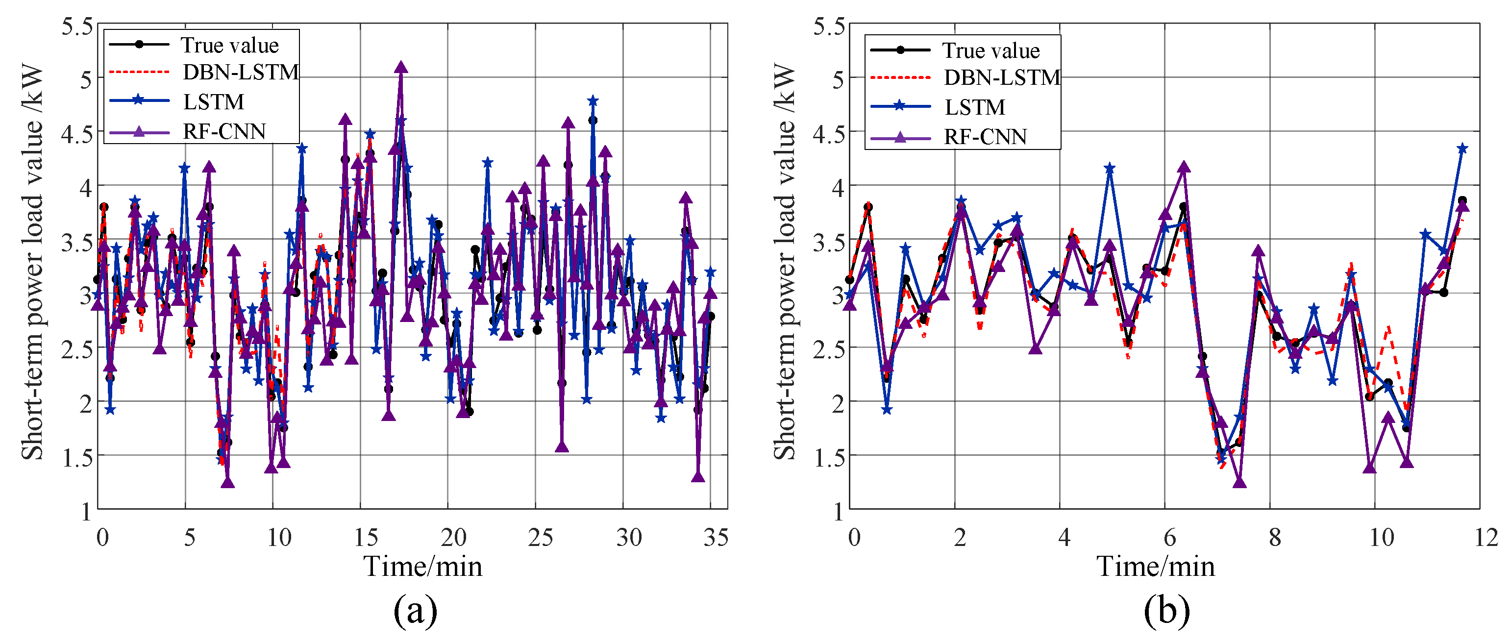
Unexpected equipment failures or scheduled maintenance may lead to abrupt short-term fluctuations in load. To evaluate the predictive performance of the model under such disturbances, artificial noise was introduced into the dataset to conduct a robustness test, with the results illustrated in Figure 18. Figure 18a presents the overall prediction results, while Figure 18b provides a zoomed-in view of the prediction over a selected time segment. The experimental results indicate that, in the single-load forecasting task, the predictions generated by the DBN–LSTM model closely match the actual values, with errors maintained within 0.1 kW, whereas the prediction errors of the conventional LSTM model reach approximately 1.0 kW. These results demonstrate that the DBN–LSTM model can maintain high prediction accuracy when facing sudden load variations, thereby exhibiting strong robustness.

The DBN-LSTM model’s key advantage lies in reducing redundant parameters, improving training efficiency and inference speed, and enhancing accuracy. By integrating DBN’s deep feature extraction with LSTM’s temporal memory, it captures complex nonlinearities and long-term dependencies in load patterns. This synergy enables superior adaptation to diverse consumption behaviors, outperforming traditional LSTM and linear models in peak load forecasting.

6.3. Optimization-Based Load Shedding Under Stability Constraints

The proposed UFLS strategy was tested on the modified IEEE 30-bus system, where total load was increased by 1.7 times and distributed proportionally among load buses. Generator set points were also adjusted.

Table 5. Standard locations and weighting coefficients.

Standard Locations	Value	Weighting	Value
${\xi }_{l,1}$	1.6508	${\omega }_{l,1}$	0.1928
${\xi }_{l,2}$	−1.4908	${\omega }_{l,2}$	0.2135
${\xi }_{l,3}$	0	${\omega }_{l,3}$	0.5937

summarizes the standard locations and weighting coefficients, while

Table 6. Estimated points of IEEE 30-bus test system.

Point Number	Active Power (MW)	Reactive Power (MVAr)
1	512.8368	145.5348
2	374.7934	106.3603
3	440.3000	124.9500

lists the three points of the $2m+1$ PEM used for load shedding analysis. These results informed the expected objective value calculation (Figure 10). Notably, the first, second, and third points correspond to positive, negative, and zero deviations from the base load, respectively, as confirmed by Table 6.

6.3.1. Parameter Sensitivity Analysis of the DGSO Algorithm

For optimization algorithms, parameter settings significantly affect the search capability and convergence performance. The DGSO algorithm mainly involves four key parameters: the population size ($NP$), the producer ratio ($PS$), the maximum number of iterations ($Iter$), and the disturbance scale (d). Each parameter contains three levels, as shown in

Table 7. Factors and levels of the orthogonal experiment.

Factor	NP (1)	PS (2)	Iter (3)	d (4)
Level 1	15	0.3	50	2
Level 2	25	0.4	100	3
Level 3	35	0.5	150	4

. If a full factorial experiment were conducted, a total of $3^4=81$ experiments would be required. To reduce the computational burden, this paper adopts an orthogonal experimental design to determine the parameter settings. With this approach, only $3^2=9$ experiments are required to effectively identify the optimal parameter combination.

Based on the experimental results, the average value $K_i$ of each factor at different levels is calculated, and the range R is further obtained. The corresponding results are presented in

Table 8. Range analysis results.

Index	NP	PS	Iter	d
$k_1$	0.320	0.326	0.323	0.323
$k_2$	0.333	0.330	0.329	0.329
$k_3$	0.327	0.325	0.328	0.328
Range R	0.013	0.005	0.006	0.006

.

Table 8 and

Table 9. $L_9\left(3^4\right)$ orthogonal table and experimental results.

Experiment	NP	PS	Iter	d	PV Margin
1	15 (1)	0.3 (1)	50 (1)	2 (1)	1.40
2	15 (1)	0.4 (2)	100 (2)	3 (2)	1.75
3	15 (1)	0.5 (3)	150 (3)	4 (3)	1.68
4	25 (2)	0.3 (1)	150 (3)	2 (1)	1.82
5	25 (2)	0.4 (2)	100 (2)	3 (2)	2.43
6	25 (2)	0.5 (3)	50 (1)	4 (3)	2.16
7	35 (3)	0.3 (1)	150 (3)	3 (2)	1.95
8	35 (3)	0.4 (2)	50 (1)	4 (3)	1.72
9	35 (3)	0.5 (3)	100 (2)	2 (1)	1.65

present the experimental results of the orthogonal design table $L_9\left(3^4\right)$ and the corresponding range analysis results. Based on the orthogonal design analysis, the optimal parameter combination is determined as $NP=25$, $PS=0.4$, $Iter=100$, and $d=3$.

Under this parameter setting, the DGSO algorithm achieves improved search capability and convergence performance, thereby obtaining a larger PV margin and enhancing the accuracy of static voltage stability assessment in power systems.

6.3.2. Performance Evaluation of DGSO-Based Optimization Under Stability Constraints

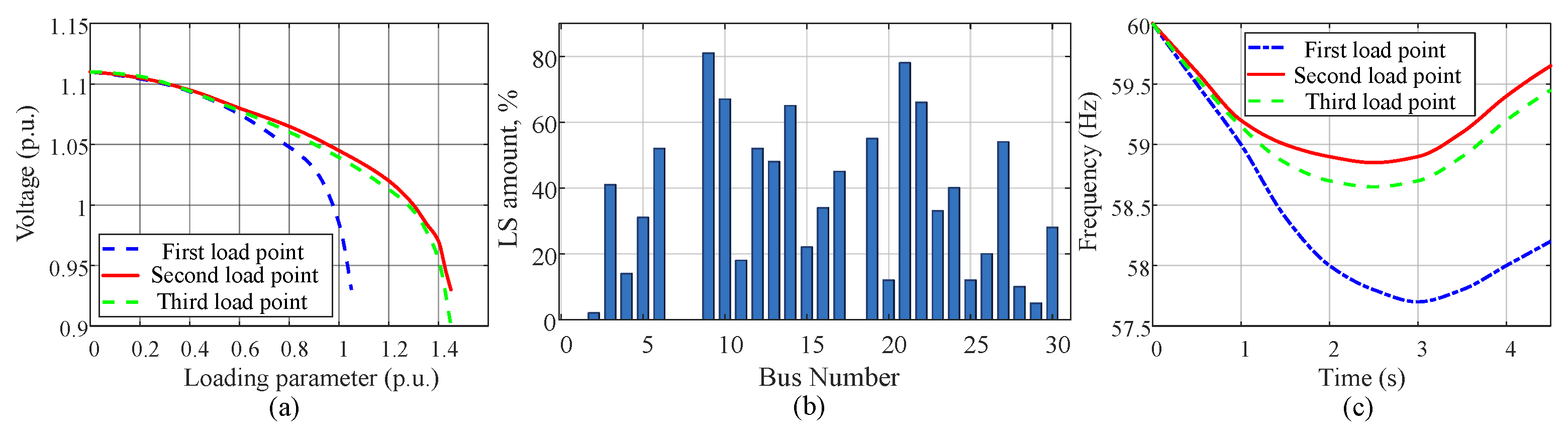
A contingency scenario is simulated in which a 200 MW generator at Bus 2 trips at $t=0.1\mathrm{s}$. Figure 19a shows the PV curves of Bus 3 under three PEM load points. As the load level increases, the bus voltage gradually decreases and approaches the voltage stability limit. A turning point appears near the critical loading condition, indicating proximity to voltage collapse. The PV margins vary under different load scenarios.

Figure 19b presents the load shedding ratios determined by the DGSO-UFLS method in the IEEE 30-bus system. Load shedding is mainly concentrated at several critical buses, indicating that the proposed method can identify appropriate shedding locations and allocate the shedding amounts effectively.

Table 10. PV margins in the modified IEEE 30-bus system.

Load Scenario	Conventional Method	Method Used in [2]	PSO Method	DGSO Method
1	1.25	1.71	1.61	1.75
2	1.46	2.38	2.14	2.43
3	1.45	2.07	1.81	2.16
Expected value	1.4136	2.0668	1.8437	2.1356

compares the PV stability margins obtained by different load shedding methods. The proposed DGSO method achieves the largest PV margins in all scenarios, with an expected value of 2.1356, outperforming the conventional and other optimization methods. This confirms that the proposed probabilistic DGSO-UFLS method can effectively enhance voltage stability while providing a more reasonable load shedding scheme.

6.3.3. Contingency Simulation and Probabilistic Load Shedding Implementation

The standard IEEE 30-bus system consists of four generators and twenty-six load buses, operating at a nominal frequency of $60\mathrm{Hz}$. At all buses, a combination of static and dynamic load models is employed. The standard locations and weighting coefficients provided in Table 5 were utilized to implement the proposed probabilistic load shedding scheme. The three load points generated from the $2m+1$ PEM are listed in

Table 11. Estimated points of the IEEE 30-bus.

Point Number	Active Power (MW)	Reactive Power (MVAr)
1	7070.11	1640.31
2	5167.01	1198.78
3	6070.10	1408.30

, with total system loads of $7070.11\mathrm{MW}$, $5167.01\mathrm{MW}$, and $6070.10\mathrm{MW}$ for points one, two, and three, respectively.

6.3.4. Stability-Driven Performance Evaluation of the DGSO-Based Scheme

A contingency involving the outage of the 1000 MW generator at bus 18 (trip at $t=0.1\mathrm{s}$) was simulated, resulting in power imbalances of 660 MW, 220 MW, and 500 MW for the first, second, and third load points, respectively.

Table 12. Expected value of determined loads for DGSO-based UFLS method in the IEEE 30-bus system.

Bus	Expected LS Amount (%)
14	100.00
30	41.37

presents the expected load shedding amounts calculated via the probabilistic method, consistently selecting load 14 across scenarios.

After a generator outage, the dynamic response of the system frequency under three load scenarios is illustrated in Figure 19c. Following the fault, the reduction in generation leads to an active power imbalance, causing a significant decline in system frequency. Among the three scenarios, the first load scenario experiences the most severe frequency drop. After selective load shedding is implemented, the system frequency in all three scenarios gradually recovers. These results indicate that an appropriate load shedding strategy can effectively suppress frequency decline and improve the dynamic stability of the power system.

7. Conclusions

This paper addresses the voltage stability challenges caused by the high penetration of renewable energy in power systems and proposes an integrated framework that combines static voltage stability assessment, power forecasting, and stability-constrained load shedding optimization. The main conclusions are summarized as follows.

(1) A low-conservatism analytical criterion for static voltage stability is proposed. The criterion has an explicit analytical form whose mathematical expression depends only on network parameters, graph topology, and power injections, without relying on the specific system size. Therefore, it can theoretically be extended to larger-scale power systems. Simulation results demonstrate that the proposed criterion can effectively evaluate the voltage stability margin under different loading conditions.

(2) A hybrid DBN–LSTM load forecasting model is developed. By combining the feature extraction capability of the DBN with the temporal modeling ability of the LSTM, the proposed model improves load forecasting accuracy. Experimental results show that, compared with RF–CNN and conventional LSTM models, the DBN–LSTM model achieves better performance in terms of MAE, RMSE, and MAPE. Statistical significance tests further verify the superiority of the proposed forecasting model.

(3) A DGSO-based load shedding strategy is proposed. By optimizing the locations and proportions of load shedding while considering load uncertainty, the proposed method effectively improves the system voltage stability margin. Simulation results on the IEEE test system show that the proposed approach significantly increases the PV margin and enhances overall system stability.

From an engineering perspective, the proposed method can be integrated with existing Energy Management Systems (EMSs) and SCADA/PMU measurement platforms to support online stability assessment and optimization decision-making. The load shedding strategy can be implemented through existing protection and control devices, demonstrating promising potential for practical applications.

Nevertheless, several limitations remain. The simulations in this study are mainly conducted on IEEE standard test systems, and further validation on larger-scale systems and real power grids is required. In addition, the performance of the DBN–LSTM forecasting model depends on the quality of historical data and the size of training samples. The computational efficiency of the DGSO algorithm in large-scale systems also requires further investigation. Future work will focus on validating and improving the proposed framework using larger test systems and real-world operational data.

References

1. Wu, F.F.; Kumagai, S. Steady-state security regions of power systems. IEEE Trans. Circuits Syst. 1982, 29, 703–711. [Google Scholar] [CrossRef]
2. Ilić, M.D. Network theoretic conditions for existence and uniqueness of steady state solutions to electric power circuits. In Proceedings of the 31st IEEE Conference on Decision and Control, Tucson, AZ, USA, 16–18 December 1992; pp. 376–381. [Google Scholar]
3. Chiang, H.D.; Baran, M.E. On the existence and uniqueness of load flow solution for radial distribution power networks. IEEE Trans. Circuits Syst. 1990, 37, 410–416. [Google Scholar] [CrossRef]
4. Miu, K.N.; Chiang, H.D. Existence, uniqueness, and monotonic properties of the feasible power flow solution for radial three-phase distribution networks. IEEE Trans. Circuits Syst. I Fundam. Theory Appl. 2000, 47, 1502–1514. [Google Scholar]
5. Dvijotham, K.; Low, S.H.; Chertkov, M. Convexity of energy-like functions: Theoretical results and applications to power system operations. In Proceedings of the IEEE Power & Energy Society General Meeting, Denver, CO, USA, 26–30 July 2015; pp. 1–5. [Google Scholar]
6. Dvijotham, K.; Chertkov, M.; Low, S. Monotone operator approach to power flow solutions. In Proceedings of the 2016 American Control Conference (ACC), Boston, MA, USA, 6–8 July 2016; pp. 1769–1775. [Google Scholar]
7. Dörfler, F.; Chertkov, M.; Bullo, F. Synchronization in complex oscillator networks and smart grids. Proc. Natl. Acad. Sci. USA 2013, 110, 2005–2010. [Google Scholar] [CrossRef] [PubMed]
8. Jafarpour, S.; Bullo, F. Synchronization of kuramoto oscillators via cutset projections. IEEE Trans. Autom. Control 2019, 64, 1920–1935. [Google Scholar] [CrossRef]
9. Jafarpour, S.; Huang, Y.; Smith, R.S.; Bullo, F. Flow and elastic networks on the n-torus: Geometry, analysis, and computation. IEEE Trans. Autom. Control 2022, 67, 2703–2718. [Google Scholar] [CrossRef]
10. Delabays, R.; Jafarpour, S.; Bullo, F. An energy based security measure for assessing vulnerability to voltage collapse. IEEE Trans. Power Syst. 2022, 37, 1347–1359. [Google Scholar]
11. Simpson-Porco, J.W.; Dörfler, F.; Bullo, F. Voltage collapse in complex power grids. Nat. Commun. 2016, 7, 10790. [Google Scholar] [CrossRef]
12. Barabanov, N.E.; Ortega, R.; Griñó, R.; Polyak, B.T. On Existence and Stability of Equilibria of Linear Time-Invariant Systems with Constant Power Loads. IEEE Trans. Circuits Syst. I Regul. Pap. 2016, 63, 114–126. [Google Scholar] [CrossRef]
13. Liu, X.; Wang, X.; Blaabjerg, F.; Chen, Z. Existence and stability of equilibrium of DC microgrid with constant power loads. IEEE Trans. Power Syst. 2018, 33, 6514–6523. [Google Scholar] [CrossRef]
14. Chen, L.; Simpson-Porco, J.W. A fixed-point algorithm for the AC power flow problem. In Proceedings of the 2023 American Control Conference (ACC), San Diego, CA, USA, 31 May–2 June 2023; pp. 4449–4456. [Google Scholar]
15. Alzubaidi, M.; Hasan, K.N.; Meegahapola, L.; Rahman, M.T. Probabilistic Voltage Stability Analysis Considering Variable Wind Generation and Different Control Modes. In Proceedings of the 31st Australasian Universities Power Engineering Conference (AUPEC) Perth, Australia, 26–30 September 2021. [Google Scholar]
16. Alzubaidi, M.; Hasan, K.N.; Meegahapola, L.; Rahman, M.T. Probabilistic Voltage Stability Assessment Considering Load and Wind Uncertainties. In Proceedings of the IEEE PES Innovative Smart Grid Technologies Asia (ISGT Asia), Brisbane, Australia, 5–8 December 2021. Paper presented at ISGT Asia 2021. [Google Scholar]
17. Huang, X.; Yan, Z. Probabilistic Static Voltage Stability Assessment for Distribution Network Considering Correlated Renewable Energy. In Proceedings of the 5th Asia Conference on Power and Electrical Engineering (ACPEE), Chengdu, China, 4–7 June 2020. Paper presented at ACPEE 2020. [Google Scholar]
18. Dong, X.; Qian, L.; Huang, L. Short-term load forecasting in smart grid: A combined CNN and K-means clustering approach. In Proceedings of the IEEE International Conference on Big Data and Smart Computing (BigComp), Jeju Island, Republic of Korea, 13–16 February 2017; pp. 119–125. [Google Scholar]
19. Veeramsetty, V.; Reddy, K.R.; Santhosh, M.; Mohnot, A.; Singal, G. Short-term electric power load forecasting using random forest and gated recurrent unit. Electr. Power Syst. Res. 2022, 210, 107999. [Google Scholar] [CrossRef]
20. Xiang, W.; Xu, P.; Fang, J.; Zhao, Q.; Gu, Z.; Zhang, Q. Multi-dimensional data-based medium-and long-term power-load forecasting using double-layer CatBoost. Energy Rep. 2022, 8, 8511–8522. [Google Scholar] [CrossRef]
21. Duan, J.; Wang, P.; Ma, W.; Tian, X.; Fang, S.; Cheng, Y.; Chang, Y.; Liu, H. Short-term wind power forecasting using the hybrid model of improved variational mode decomposition and Correntropy Long Short-term memory neural network. Energy 2021, 214, 118980. [Google Scholar] [CrossRef]
22. Kim, N.; Park, H.; Lee, J.; Choi, J.K. Short-term electrical load forecasting with multidimensional feature extraction. IEEE Trans. Smart Grid 2022, 13, 2999–3013. [Google Scholar] [CrossRef]
23. Jiang, L.; Wang, X.; Li, W.; Wang, L.; Yin, X.; Jia, L. Hybrid multitask multi-information fusion deep learning for household short-term load forecasting. IEEE Trans. Smart Grid 2021, 12, 5362–5372. [Google Scholar] [CrossRef]
24. Zufferey, T.; Renggli, S.; Hug, G. Probabilistic state forecasting and optimal voltage control in distribution grids under uncertainty. Electr. Power Syst. Res. 2020, 188, 106562. [Google Scholar] [CrossRef]
25. Sanaye-Pasand, M.; Seyedi, H. Centralized adaptive load shedding methods to enhance power system voltage stability margins. IEEE Trans. Electr. Electron. Eng. 2008, 3, 669–679. [Google Scholar] [CrossRef]
26. Jonsson, M. Protection Strategies to Mitigate Major Power Systems Breakdowns; Chalmers Tekniska Hogskola: Göteborg, Sweden, 2003. [Google Scholar]
27. Hafez, A.A.; Hatata, A.Y.; Abdelaziz, A.Y. Multiobjective particle swarm for optimal load shedding remedy strategies of power system. Electr. Power Components Syst. 2019, 47, 1651–1666. [Google Scholar] [CrossRef]
28. Western Electricity Coordinating Council. WECC Coordinated Off-Nominal Frequency Load Shedding and Restoration Requirements; Western Electricity Coordinating Council: Salt Lake City, UT, USA, 2005. [Google Scholar]
29. Crossley, P.; Karlsson, D. System protection schemes in power networks: Existing installations and ideas for future development. In Proceedings of the Seventh International Conference on Developments in Power System Protection (IEE), Amsterdam, The Netherlands, 9–12 April 2001; IET: Hertfordshire, UK, 2001; pp. 450–453. [Google Scholar]
30. Seyedi, H.; Sanaye-Pasand, M. Design of new load shedding special protection schemes for a double area power system. Am. J. Appl. Sci. 2009, 6, 317–327. [Google Scholar] [CrossRef]
31. Seyedi, H.; Sanaye-Pasand, M. New centralised adaptive load-shedding algorithms to mitigate power system blackouts. IET Gener. Transm. Distrib. 2009, 3, 99–114. [Google Scholar] [CrossRef]
32. Marzband, M.; Moghaddam, M.M.; Akorede, M.F.; Khomeyrani, G. Adaptive load shedding scheme for frequency stability enhancement in microgrids. Electr. Power Syst. Res. 2016, 140, 78–86. [Google Scholar] [CrossRef]
33. Hoseinzadeh, B.; Amini, M.H.; Bak, C.L. Centralized load shedding based on thermal limit of transmission lines against cascading events. In Proceedings of the 2017 IEEE Power & Energy Society General Meeting, Chicago, IL USA, 16–20 July 2017; IEEE: Piscataway, NJ, USA, 2017; pp. 1–5. [Google Scholar]
34. Sadati, N.; Amraee, T.; Ranjbar, A. A global particle swarm-based-simulated annealing optimization technique for under-voltage load shedding problem. Appl. Soft Comput. 2009, 9, 652–657. [Google Scholar] [CrossRef]
35. Tung, Y.K.; Yen, B.C. Hydrosystems Engineering Uncertainty Analysis; American Society of Civil Engineers: ASCE: Reston, VA, USA, 2005. [Google Scholar]
36. Su, C.-L. Probabilistic load-flow computation using point estimate method. IEEE Trans. Power Syst. 2005, 20, 1843–1851. [Google Scholar] [CrossRef]
37. Zhang, X.; Chan, K.W.; Wang, H.; Zhou, B.; Wang, G.; Qiu, J. Multiple group search optimization based on decomposition for multi-objective dispatch with electric vehicle and wind power uncertainties. Appl. Energy 2020, 262, 114507. [Google Scholar] [CrossRef]
38. Huang, J.; Ding, X.; Jin, D.; Liu, Z. Static voltage stability analysis of integrated smart energy systems. Front. Energy Res. 2024, 12, 1500830. [Google Scholar] [CrossRef]
Figure 1. The structure of the DBN.
Jlpea 16 00011 g001
Figure 2. The schematic diagram of the LSTM multilayer structure.
Jlpea 16 00011 g002
Figure 3. Structure diagram of the LSTM prediction model.
Jlpea 16 00011 g003
Figure 4. Overall framework diagram of the DBN-LSTM prediction model.
Jlpea 16 00011 g004
Figure 5. The structure of the DBN-LSTM.
Jlpea 16 00011 g005
Figure 6. Randomly determine the producer member’s step length and specify the zero, right, and left positions.
Jlpea 16 00011 g006
Figure 7. The process of scrounging.
Jlpea 16 00011 g007
Figure 8. Matrix A within the discrete search domain.
Jlpea 16 00011 g008
Figure 9. Generation process at the second stage of the head angle.
Jlpea 16 00011 g009
Figure 10. The flowchart of probabilistic DGSO implementation.
Jlpea 16 00011 g010
Figure 11. IEEE bus topology diagram. (a) The 14-bus system. (b) The 30-bus system. (c) The 57-bus system.
Jlpea 16 00011 g011
Figure 12. Contour of voltage stability limit estimation for IEEE test systems. (a) The 14-bus system. (b) The 30-bus system. (c) The 57-bus system.
Jlpea 16 00011 g012
Figure 13. Bus voltage magnitudes for IEEE 30-bus system at base loading condition. True voltage magnitudes are shown in Jlpea 16 00011 i001 and approximate values are shown in Jlpea 16 00011 i002. Voltage magnitude upper and lower bounds as given in Theorem 1 are shown in .
Jlpea 16 00011 g013
Figure 14. Bus voltage angles for IEEE 30-bus system at base loading condition. True voltage angles are shown in Jlpea 16 00011 i001 and approximate values are shown in Jlpea 16 00011 i002. Voltage angle upper and lower bounds as given in Theorem 1 are shown in .
Jlpea 16 00011 g014
Figure 15. The iteration processes of the proposed algorithm. (a) Convergence when τ < 1 . (b) Divergence when τ 1 .
Jlpea 16 00011 g015
Figure 16. Training and validation loss curves of the DBN–LSTM model over epochs.
Jlpea 16 00011 g016
Figure 17. Comparison of predicted load and actual load. (a) Short-term load forecasting within a selected time window (minutes). (b) Daily load forecasting over a 24 h period (hours).
Jlpea 16 00011 g017
Figure 18. Prediction results of short-term power load after introducing interference. (a) Forecast results. (b) Enlarged results.
Jlpea 16 00011 g018
Figure 19. Load shedding (LS). (a) PV curves of Bus 3 under three PEM load points. (b) Determined load shedding percentages of buses using the proposed DGSO-UFLS scheme. (c) System frequency responses following the outage of the generator at Bus 2 under three load points.
Jlpea 16 00011 g019