Abstract
In the context of aging populations, it has become necessary to develop new methods and devices for the daily home-based self-rehabilitation of elderly people. To this end, this paper proposes and evaluates the use of an easy-to-use single battery-powered device including a 3D accelerometer and a 3D gyroscope, where light algorithms, such as the complementary filter and the Kalman filter, are implemented to estimate the elbow joint angle. During experiments, a robotic arm and a human arm were used to obtain an error interval for each tested algorithm; the robotic arm allows for reproducible movements and reproducible results, which allows us to independently verify the impact of parameters such as the sensor’s movement speed on the algorithm precision. The experimental results show that the algorithm that uses only accelerometer data is one of the most relevant since it allows us to obtain a Root Mean Square Error between 1.83° and 5.52° at a sensor data rate of 100 Hz, which is similar to the results obtained using the data fusion algorithms tested. Nevertheless, it has a lower power consumption since it requires only 58 cycles when using an ARM Cortex-M4 processor (which is lower than that of the other data fusion algorithms tested by a factor of at least two), and it does not necessitate the additional sensor required by the other data fusion algorithms tested (such as a gyroscope or a magnetometer). The algorithm using only accelerometer data also seems to be the algorithm with the lowest power consumption and should be preferred. Moreover, its power consumption can be reduced by more than the increase in the error when reducing the rate of the data output by the sensor. In this work, a reduction in the data rate from 100 Hz to 10 Hz increased the RMSE by a factor of 1.8 but could reduce the power consumption associated with the sensor and the algorithm’s computation by a factor of 10. Finally, the experimental results show that the higher the speed of the sensor’s motion, the higher the error obtained using only accelerometer data. Nevertheless, the algorithm that uses only accelerometer data remains well suited to rehabilitation exercises or mobility evaluations since the speed of the sensor’s movement is also moderate.
1. Introduction
In most countries of the Organization for Economic Co-operation and Development (OECD), an aging population has been observed for many years, and this phenomenon continues to increase. In 2021, according to statistics from the OECD published in 2023 [1], 18% of the population of OECD member countries was at least 65 years old, and 4.8% was at least 80 years old. According to the OECD’s projections for 2050, 27% of this population will be at least 65 years old, and 9.8% will be 80 years old or older. This proportion is expected to be especially high in Korea, Japan, Italy, Greece, and Portugal, where more than a third of the population will be older than 65 (and 10% older than 80) years old by 2050.
Population aging is accompanied by an increase in healthcare costs due to the increased need for medical care and specialized infrastructure for elderly care. Thus, it is necessary to increase the autonomy of elderly persons so that they can receive their daily care at home [2]. This implies an evolution in medical devices and especially their miniaturization to enable their easy use at home. Research has also been conducted on the design of devices for biomedical signal acquisition that can be used at home, such as electrocardiograms (ECGs), which reflect the electrical activity of the heart [3], or photoplethysmograms (PPGs), which allow us to deduce heart rate and blood oxygen levels [4]. Other works have also been carried out to reduce the risk of falling when walking in everyday life, such as placing a three-axis accelerometer on the thorax [5] or equipping a wheelchair with sensors and cameras to detect unusual events and prevent possible falls or accidents [6].
In this context, people’s rehabilitation must evolve to offer them the possibility of carrying out their daily exercises at home in complete autonomy while evolving their mobility. This has become possible due to the miniaturization of low-cost embedded systems, allowing for movement tracking and providing user feedback in addition to the appropriate medical monitoring. Many systems developed for rehabilitation consist of monitoring a person’s movement. In the literature, these systems have mainly used methods based on inertial sensors [7,8,9,10]. However, they can also be based on the measurement of surface electromyography (sEMG) signals [11,12,13,14]. Unfortunately, these are less integrated and require more power-consuming electronic front-ends compared to those for inertial sensors, in addition to requiring heavy algorithms such as artificial neural networks (ANNs). Methods based on inertial sensors, which are usually composed of a three-axis accelerometer and a three-axis gyroscope, use at least two devices fixed to the human body or a single device coupled with a mechanical solution, such as in [15], which uses a mechanical system based on a potentiometer to measure the movements of a patient’s elbow. These research works have led to marketable solutions such as that proposed by Xsens [16], which embeds a three-axis magnetometer into each device in addition to a three-axis accelerometer and a three-axis gyroscope. This has begun to be considered for rehabilitation, even though it was initially developed for motion capture, entertainment, sports, and machine control.
The purpose of these devices is to precisely measure the joint angle between two limbs—for example, the angle of the elbow or the absolute orientation of a limb. However, accelerometer data contain important noise and bias that can change over time, whereas gyroscope data contain important bias. Magnetometers can be used with inertial sensors too but are sensitive to ambient magnetic fields. Therefore, these sensors need to be calibrated, and their data must be fused to compensate for their error and obtain a relevant assessment of the targeted angle or absolute orientation. For this, specific algorithms can be used, such as the complementary filter (CF) or the Kalman filter (KF).
However, the use of a specific filter does not guarantee a relevant estimation. Indeed, among the examples given here concerning the elbow angle, ref. [17] studies the kinematics of the whole body using several sensors and retains a maximum Root Mean Square Error (RMSE) of 5° by using the KF. Another example is [18], where an RMSE higher than 20° is obtained despite calibration and the use of the KF.
Nevertheless, better results have also been obtained. In [19], a KF is used with a specific static calibration method which allows the authors to reach an RMSE of 2.7°. Reference [20] obtains an RMSE of 2.62° using the KF too. In [21], the dimensions of people’s bodies are measured before proceeding to the experiments, which allows the authors to obtain an RMSE of 2.4°. Moreover, it should be noted that the RMSE value does not foresee the correlation of the estimated angles. Indeed, it generally stays high when using the KF even in the case of a high RMSE (in [17], the correlation is higher than 0.95 for an RMSE higher than 20°). Finally, ref. [22], which studies the knee joint angle during walking using two magneto-inertial devices (and also includes a magnetometer in addition to an accelerometer and a gyroscope), obtains an RMSE between 0.5° and 3° in addition to a correlation between 0.97 and 0.99.
The accuracy of the CF is generally close to the accuracy of the KF. Thanks to its particular implementation of the CF, ref. [23] obtained an RMSE between 1.8° and 2.16° for all experiment sessions. Equally, ref. [24], which studied the bilateral knee joint angles using four inertial devices simultaneously, achieves an RMSE between 1.62° and 3.30°.
Finally, in the context of daily home-based self-rehabilitation, the patient must execute movements without the help of other people. It is also necessary to provide a solution that is easy to set up, simple to use, and not constraining to maintain (especially as regards battery charging for devices). In addition, it is necessary for the device to be minimally intrusive and inexpensive but accurate enough to obtain relevant data. Thus, small and low-cost sensors, such as Micro-Electromechanical Systems (MEMSs), which can be integrated into compact devices, must be preferred. Moreover, the solution must be low-power enough to prevent the patient from frequently being disturbed by battery issues during exercises. Finally, the number of devices fixed to the human body must also be as low as possible to offer the most seamless user experience.
Thus, an ideal device for joint rehabilitation would be composed of a single band-type device, with a limited number of sensors to limit the power consumption and cost. This device should be place on a limb without necessitating precise positioning thanks to a simple attachment system, such as Velcro straps. Moreover, it could communicate, for instance, via Bluetooth with the patient’s cell phone or with a dedicated smart device to provide feedback to the user. The smart device would also give instructions to the patient so that they could correct their movements, follow simple and adapted exercises, and visualize the evolution in limb mobility. In addition, the smart device should allow a healthcare professional to follow the patient’s progress by securely transmitting the data to the cloud. Finally, the sensor calibration process must be as simple as possible.
The work presented in this paper also aims to quantify the orientation error obtained using a three-axis accelerometer and/or a three-axis gyroscope and light algorithms embedded into a single device during rehabilitation movements, such as elbow flexion/extension, as illustrated in Figure 1. In order to evaluate the impact on the precision of the angular speed and sensor placement only (which can be linked to the sensor’s movement speed), the algorithms are firstly evaluated using a robotic arm that can move in a reproducible manner. Next, they are evaluated using a human arm to determine the achievable performance for real cases. Finally, the sensor type, the number of arithmetic operations required by each algorithm, and the sensor data rate are investigated in particular since the rehabilitation device’s power consumption highly depends on these properties.
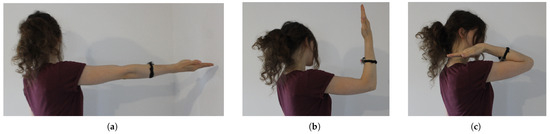
Figure 1.
Depiction of human arm flexion/extension movements: (a) an unfolded arm (an elbow angle of about 180°); (b) the arm with an elbow angle of 90°; and (c) the arm folded to its maximum bend (an elbow angle of about 30°).
Thus, the aim of this work is to identify the most relevant sensors and algorithms, in terms of their precision and power consumption, in the context of limb rehabilitation and the evaluation of their mobility. To allow for this, Section 2 presents a device which has been fixed to the arm during experiments and the hardware it includes, such as the sensor. This is followed by a presentation of the kinematics associated with elbow angle estimation and the algorithms tested in this paper for estimating this value using accelerometer and gyroscope data. The outcome metrics and the configurations tested are also presented. Next, the results are presented in Section 3 and discussed in Section 4. The discussions notably include the algorithm performance compared to the number of arithmetic operations required but also the sensor data rate, the angular speed during motion, and the sensor–joint distance (and also the sensor’s movement speed). Finally, our results are compared with those from other works.
2. Materials and Methods
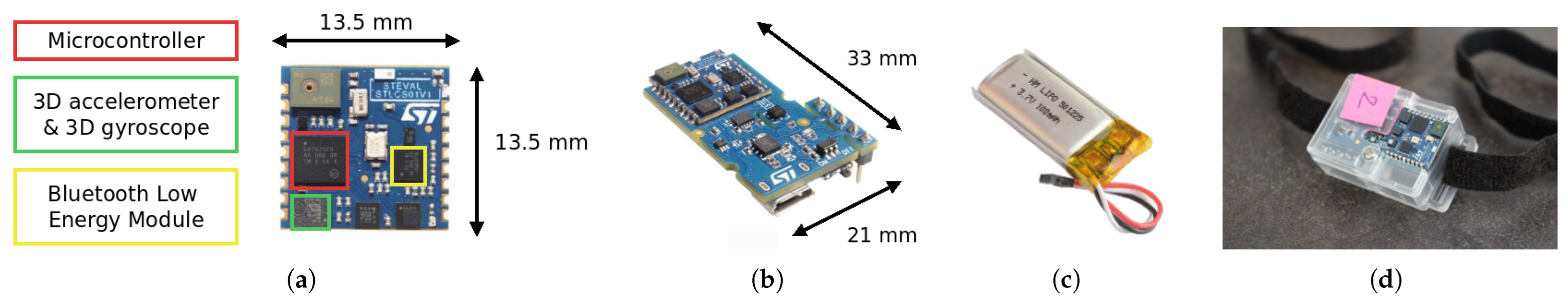
The experiments were conducted using the SensorTile development kit (STDK) from STMicroelectronics shown in Figure 2. This includes the SensorTile reference design board (STRDB), which mainly embeds the Bluetooth Low Energy (BLE) network processor BlueNRG-MS from STMicroelectronics; the ARM Cortex-M4 32-bit microcontroller STM32L476; the iNEMO inertial module LSM6DSL, including a 3D gyroscope; and the ultra-compact high-performance module LSM303AGR, including an ultra-low-power 3D accelerometer. The STDK also includes the SensorTile cradle board (STCB) onto which the STRBD has been soldered. The STCB board allows the STRBD to be supplied by a battery provided in the STDK in addition to allowing the battery to be charged through a micro USB connector. Moreover, the STDK includes a plastic case onto which the STRBD, the STCB, and the battery were mounted to create the inertial device used during the experiments. Finally, a Velcro bandstrip was added to fix the device to the arm.
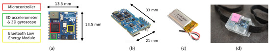
Figure 2.
SensorTile development kit used during experiments: (a) the SensorTile reference design board embedding a BLE module, an ARM Cortex-M4 microcontroller, and inertial sensors; (b) the SensorTile cradle board for programming and battery supply of the SensorTile reference design board; (c) a 100 mAh LiPO battery; and (d) the SensorTile boards and the battery in the plastic box fixed to the arm using Velcro during the experiments.
2.1. Kinematics
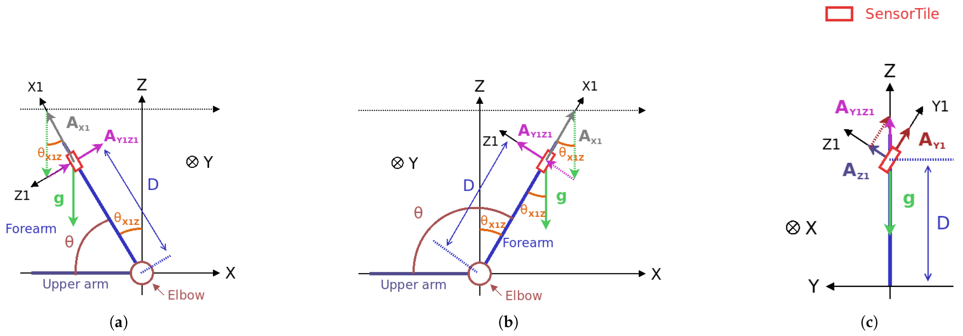
The elbow joint angle can be determined with help of Figure 3, where the arm is represented by a blue thick line. In this figure, the elbow joint is placed at the coordinates (0,0,0) of the XYZ coordinate system, and the upper arm is considered to be parallel to the ground (which is true when elbow rehabilitation exercises are performed on a table). It is also assumed that the elbow introduces a Y-axis pin joint between the forearm and the upper arm. Thus, possible forearm movements are only rotations around the Y axis and so are limited to the XZ plane.
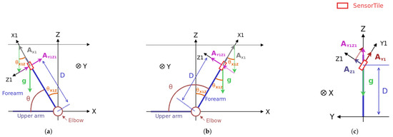
Figure 3.
A kinematic diagram for the elbow joint angle estimation assuming the upper arm in the XY plane parallel to the ground: (a) an XZ-plane diagram when the part of related to gravity is negative; (b)an XZ-plane diagram when the part of related to gravity is positive; and (c) a YZ-plane diagram.
2.1.1. The Accelerometer
During the experiments proposed here, the SensorTile inertial device is fixed to the forearm at a distance D from the elbow. It is equally fixed to the coordinate system formed by the X1, Y1, and Z1 axes. For these conditions and assuming that the part of the Z1 coordinate of the sensor acceleration related to motion is negligible compared to that due to gravity (with a stationary sensor or one subjected to a slow enough movement), the estimate of the elbow joint angle from the accelerometer data is given by
where is the acceleration measured on the Z1 axis, is the estimate of the angle between the X1 and Z axis using the accelerometer data, and is the sign function. For a discrete time system such as a system built around a microcontroller, this equation becomes
with n as the discrete time variable.
According to Figure 3, the angle is an image of the sensor’s orientation with respect to the gravitational acceleration vector . Thus, , which is the estimate of from the accelerometer data, can be computed as follows:
where , , and are the acceleration data provided by the SensorTile 3-axis accelerometer (filtered using a 2 Hz low-pass filter), and is the modulus of the measured acceleration vector projected into the Y1Z1 plane (this allows us to take into account a rotation around the X1 axis of the sensor due, for instance, to its misplacement, as visible in Figure 3c [25]). The estimate of from the accelerometer data only can also be obtained using Equations (2) and (3).
2.1.2. The Gyroscope
Assuming here that the SensorTile’s orientation relative to the arm implies that the Y axis and the Y1 axis are collinear, the angle can be estimated as follows:
where is the angular velocity around the X1 axis measured using the SensorTile 3-axis gyroscope and filtered with a 2 Hz low-pass filter. This equation can be written in discrete time using the trapezoidal rule as follows:
where is the output data rate of the system. To initialize , it is possible to use the estimate obtained from the accelerometer data when there is no movement or to impose a starting position (e.g., the arm is fully extended before beginning the rehabilitation exercise).
2.2. Data Processing
In addition to these two estimations, three other light estimations algorithms were considered in this work: a basic Gyroscope Bias Correction Algorithm (CG), a complementary filter (CF), and a Kalman filter (KF).
2.2.1. The Gyroscope Bias Correction Algorithm
The main issue with gyroscope data is their bias. For example, the angular velocity around the Y1 axis measured using a gyroscope can basically be written as follows:
where is the real angular velocity around the Y1 axis, and is the offset in the gyroscope’s angular velocity associated with the Y1 axis.
However, offsets in the gyroscope’s angular velocity are sensitive to several factors, such as the speed and the direction of movement. Nevertheless, this offset can be considered constant in the context of rehabilitation since rehabilitation movements are generally followed by the opposite movements and they are not made at a chaotic speed. In this case, is equal to
and can be written as follows:
since can be considered equal to a constant . For this reason, the estimate of , when the Gyroscope Bias Correction Algorithm (GBCA) is used, is computed as follows:
In this paper, the parameter was optimized to obtain the best results.
2.2.2. The Complementary Filter
The complementary filter (CF) is a simple filter which enables an estimation from several estimations using a weighted arithmetic mean. The estimate of (when the complementary filter is considered) is computed here from the estimate (obtained with accelerometer data) and the estimate (obtained with gyroscope data including the bias correction). It can also be written as follows:
where the corrected weight of the gyroscope is a real number between 0 and 1. In this paper, the parameter was optimized to obtain the best results.
2.2.3. The Kalman Filter
The Kalman filter (KF) is an implementation of the Bayes filter which assumes that the treated problem is in accordance with the Markov rule (the future evolution of a Markov chain depends on the past only through the present state). It is therefore a loop including a prediction step followed by a correction step, which can be written as shown in Figure 4.
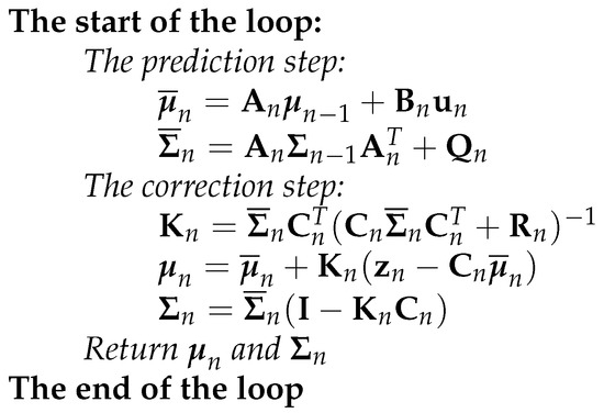
Figure 4.
Kalman filter algorithm.
For the prediction step, with is the predicted system state vector at the discrete time n; with is the corrected system state vector at the discrete time ; and with is the control vector at the discrete time n. (resp., ) links the previous corrected state (resp., the command ) to the current predicted state . In addition, is the current predicted covariance error, is the previous corrected covariance error, and is the current covariance in the process noise. Finally, is the transpose of .
For the correction step, is the optimal Kalman gain, is the measurement model, is the transpose of , is the covariance matrix of the measurement noise, and is the measurement at the discrete time n. A more advanced description of this algorithm was presented in [26].
In this work, the vectors are uni-dimensional to lighten the Kalman filter as much as possible (). In addition, gyroscope data are used in the prediction step as the control vector and accelerometer data are used in the correction step as the measurement vector . This allows the advantages of both sensors to be combined (the angles extracted from the gyroscope data have drift but are low-noise, and the angles extracted from the accelerometer data are noisy but have low drift). The vectors and are also defined as follows:
Moreover, since the data from the 3-axis gyroscope and the 3-axis accelerometer are considered independent from each other and between sensor axes and since gyroscope data must be integrated to translate the measured angular velocity into an angle, the transition matrices , , and used in this work are
where is the identity matrix.
In addition, the sensor noise is considered Gaussian and uncorrelated with each other in this work. Thus, the covariance in the process noise and the covariance matrix of the measurement noise were defined as follows:
where is the variance in the noise associated with the angular velocity measured by the gyroscope around the axis, and is the variance in the noise associated with the angle extracted from the accelerometer data. In this paper, both parameters were optimized to obtain the best results.
Finally, the corrected state is also of the form
where is the estimate of obtained with the help of the Kalman filter.
2.3. The Experiments
To evaluate the best possible performance in addition to the impact of the angular speed and the sensor placement in a reproducible manner for each algorithm, the algorithms were first evaluated with a robotic arm. Next, they were evaluated with a human arm to determine the achievable performance during real rehabilitation exercises.
Thus, the robotic arm was implemented to mimic flexion–extension movement of the elbow with precise control over this movement. This robotic arm is shown in Figure 5. Concerning the movements made by the human arm, they consist of flexion–extension movements of the arm in the sagittal plane, with the starting position shown in Figure 6.
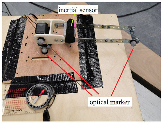
Figure 5.
Acquisition of movement of the robotic arm using optical markers and the tested inertial device.
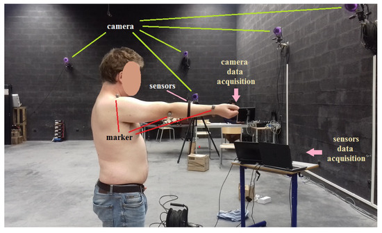
Figure 6.
Acquisition of movement of the human arm using an infrared camera system, the required optical markers, and the tested inertial device.
As shown in Figure 5 and Figure 6, a single SensorTile device, embedding an accelerometer, a gyroscope, a Bluetooth module, and a battery as described previously, was placed on the robotic arm and on the human arm. The data were collected on a computer using Bluetooth at a rate of about 100 Hz, and the five estimates of the elbow joint angle were computed with the help of MATLAB 2024a. Finally, the results were compared with the very accurate estimation obtained using an infrared motion capture system, which required optical markers.
2.4. The Comparison Metrics
Three metrics are generally used to evaluate an angle estimation algorithm—(1) the Root Mean Square Error (RMSE), (2) the Standard Deviation (STD) in the error, and (3) the correlation with the real angle—with the error computed using the real angle as a reference. This reference angle must also be accurately estimated.
In this work, the reference elbow joint angle was determined using a high-precision motion capture system from Qualisys Motion Capture System which had an output data rate of 100 Hz. For this reason, optical markers were placed on the robotic arm and the human arm as shown in Figure 5 and Figure 6. The angle error induced by the motion capture system was evaluated to less than 0.1° when there was no movement and to less than 0.5° during movements.
Thus, after synchronization of the data from the SensorTile and the motion capture system, the error induced by each tested light algorithm was estimated for each discrete time n as follows:
where is replaced by the estimate of the elbow joint angle , , , , or according to the studied algorithms.
Considering a number of samples N, the RMSE and the STD of the error were determined for each acquisition as conventional in the literature using
and
where is the mean error computed as follows:
Finally, the sample correlation coefficient r between and was computed as follows:
where is the mean value of , computed as follows:
and is the mean value of , computed as follows:
2.5. The Analyzed Parameters
As shown in Table 1, the five joint angle estimation methods were tested in 8 configurations: 5 for the robotic arm and 3 for the human arm. These various configurations of each arm were used to evaluate the impact on the accuracy of the average angular speed (during movements) and the distance between the sensor and the elbow joint. The tested angular speeds were about 30°/s, 60°/s, and 100°/s for the robotic arm and 80°/s and 220°/s for the human arm. The tested sensor–joint distances were 19 cm, 11.5 cm, and 6 cm for the robotic arm and 21 cm and 11 cm for the human arm. Moreover, the angle span is 180° for the robotic arm but about 150° only for the human arm since human tissues and bones do not allow for full flexion of the arm. Finally, it should be noted that configurations II and VI are the closest to the targeted rehabilitation use case since they involve a medium speed (60–80 °/s) and a sensor joint–distance of about 20 cm. Their results are also discussed in detail.

Table 1.
Tested configurations.
3. Results
The RMSE, the STD in the error, and the correlation obtained during the experiments are given for each configuration in Table 2, Table 3 and Table 4, respectively. It appears that the use of the gyroscope data without bias correction leads to the worst results in terms of the RMSE and the STD in the error. However, the correlation stays higher than 98%. The relevance of correlation in the literature to algorithm comparisons should also be questioned.
Table 2.
The RMSE obtained for the 8 configurations with the 5 algorithms.
Table 3.
The STD in the error obtained for the 8 configurations with the 5 algorithms.
Table 4.
The correlation with the reference obtained for the 8 configurations with the 5 algorithms.
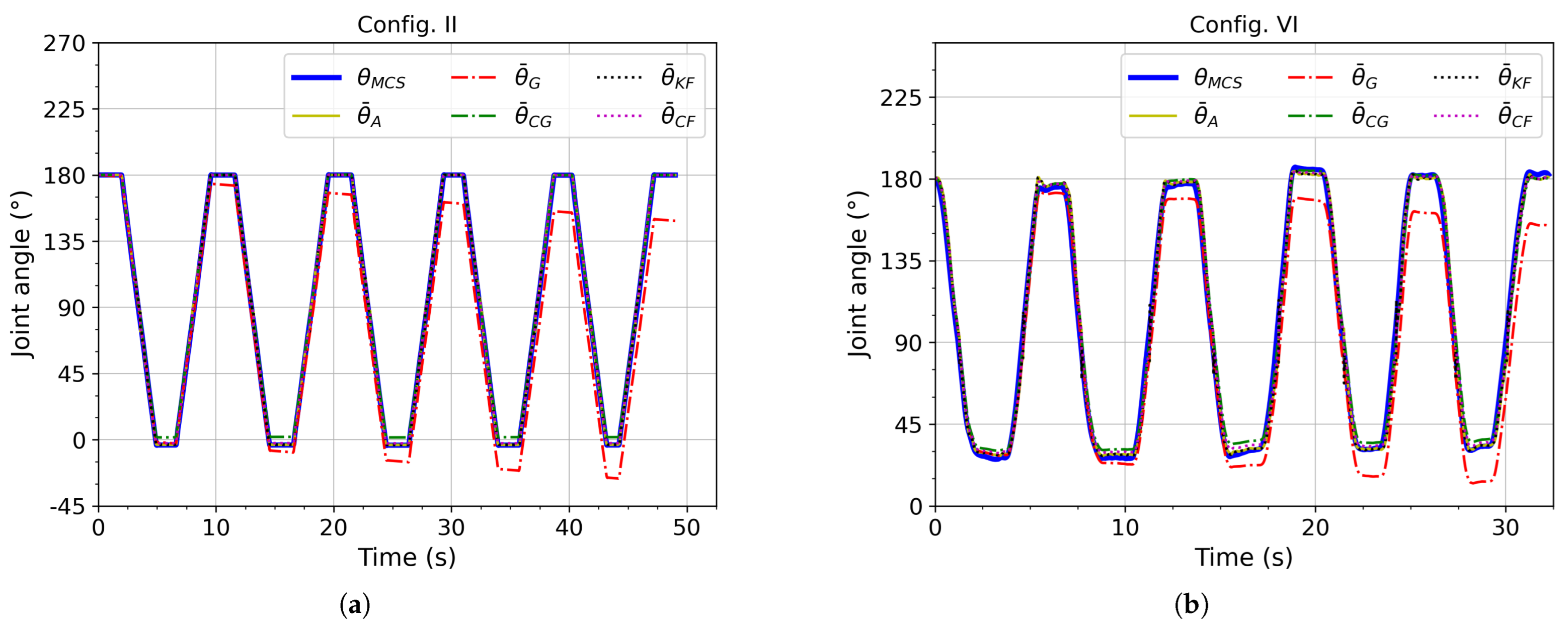
Examples of the angle estimations obtained for each algorithm in the time domain are shown in Figure 7a (resp., Figure 7b) for configuration II (resp., VI). The drift in (the estimate from the gyroscope data without drift correction) can be seen in both figures and clearly explains the bad results in terms of the RMSE and the STD in the error. Nevertheless, besides the drift, the shape of stays similar to that for , which explains the good correlation.
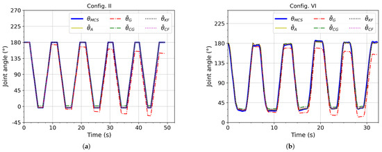
Figure 7.
Examples of estimated elbow–joint angles: (a) configuration II (robotic arm); (b) configuration VI (human arm).
Moreover, the RMSE obtained with the human arm is, as expected, higher than that obtained with the robotic arm. Indeed, the elbow’s position is not fixed during the experiments with the human arm. Nevertheless, during a rehabilitation exercise or mobility evaluation of the elbow joint, the elbow is generally placed on a table, which fixes the arm’s position. It can be deduced that the results obtained during real rehabilitation exercises would be between those obtained with the robotic arm and those obtained with the human arm. Considering configurations II and VI, the RMSE should be also between 1.69° and 5.62°.
Finally, as shown in Figure 7a (configuration II), the movements of the robotic arm are very regular, as expected, compared with those of the human arm shown in Figure 7b (configuration VI). This regularity validates the use of the robotic arm to evaluate the impact of the average angular speed during motion and the sensor–joint distance without it being affected by uncontrolled movements and also in a reproducible manner.
4. Discussion
4.1. The Algorithms’ Accuracy, Computing Costs, and Power Consumption
The results in terms of the RMSE shown in Table 2 indicate that the algorithms using only accelerometer data, the complementary filter, and the Kalman filter lead to the best results and are very close (1.69–1.83° for configuration II and 5.20–5.52° for configuration VI). These are followed by the algorithm that uses the bias-corrected gyroscope data, which can achieve an RMSE twice as high. Finally, as discussed previously, the least accurate algorithm is the one that uses the gyroscope data without bias correction since this leads to an RMSE up to ten times higher compared to that of the most accurate algorithms.
However, the algorithms using only accelerometer data, the complementary filter, and the Kalman filter do not require the same type and the same number of arithmetic operations, as shown in Table 5. Considering the number of cycles required by an ARM Cortex-M4 processor to compute the results of each elementary arithmetic operation shown in Table 6, the total number of cycles required for each method is given in Table 7 (an ARM Cortex-M4 processor was implemented in the STDK used during the experiments). Since the energy consumption of a processor designed with CMOS technology is directly proportional to the number of elapsed cycles [27,28], the algorithm that uses only accelerometer data should lead to a 1.6 to 2.1 times lower energy consumption compared to that with the complementary filter and the Kalman filter. It should also be preferred when the three algorithms have the same performance in terms of the RMSE.
In addition to the energy consumption associated with computing the estimates, the sensor’s power consumption should be considered too. Indeed, a gyroscope usually has a power consumption higher than that of an accelerometer. For instance, considering an output data rate of about 50 Hz and low-power mode, the LSM6DSL gyroscope has a power consumption of 477 μW [29], whereas the LSM303AGR accelerometer’s power consumption is only 13.9 μW [30] (the LSM6DSL also has an accelerometer but consumes 45 μW under the same conditions). Thus, the use of a gyroscope should be avoided for the targeted use case where only one low-power and low-cost battery-supplied device is fixed to the extremities of the limb since a gyroscope can have a power consumption at least 10 times higher than that of the accelerometer.
Another way to reduce the power consumption is to reduce the rate of the data output by the sensor. Indeed, a reduction in the output data rate allows us to increase the time for which the sensor is powered down. For instance, the LSM6DSL accelerometer has a power consumption of 8.1, 16.2, and 45 μW for output data rates of 1.6, 12.5, and 52 Hz, respectively (the power consumption versus the output data rate increases linearly). About the LSM303AGR accelerometer, it has a power consumption in normal mode of 6.66 and 22.7 μW for output data rates of 1 and 50 Hz, respectively.
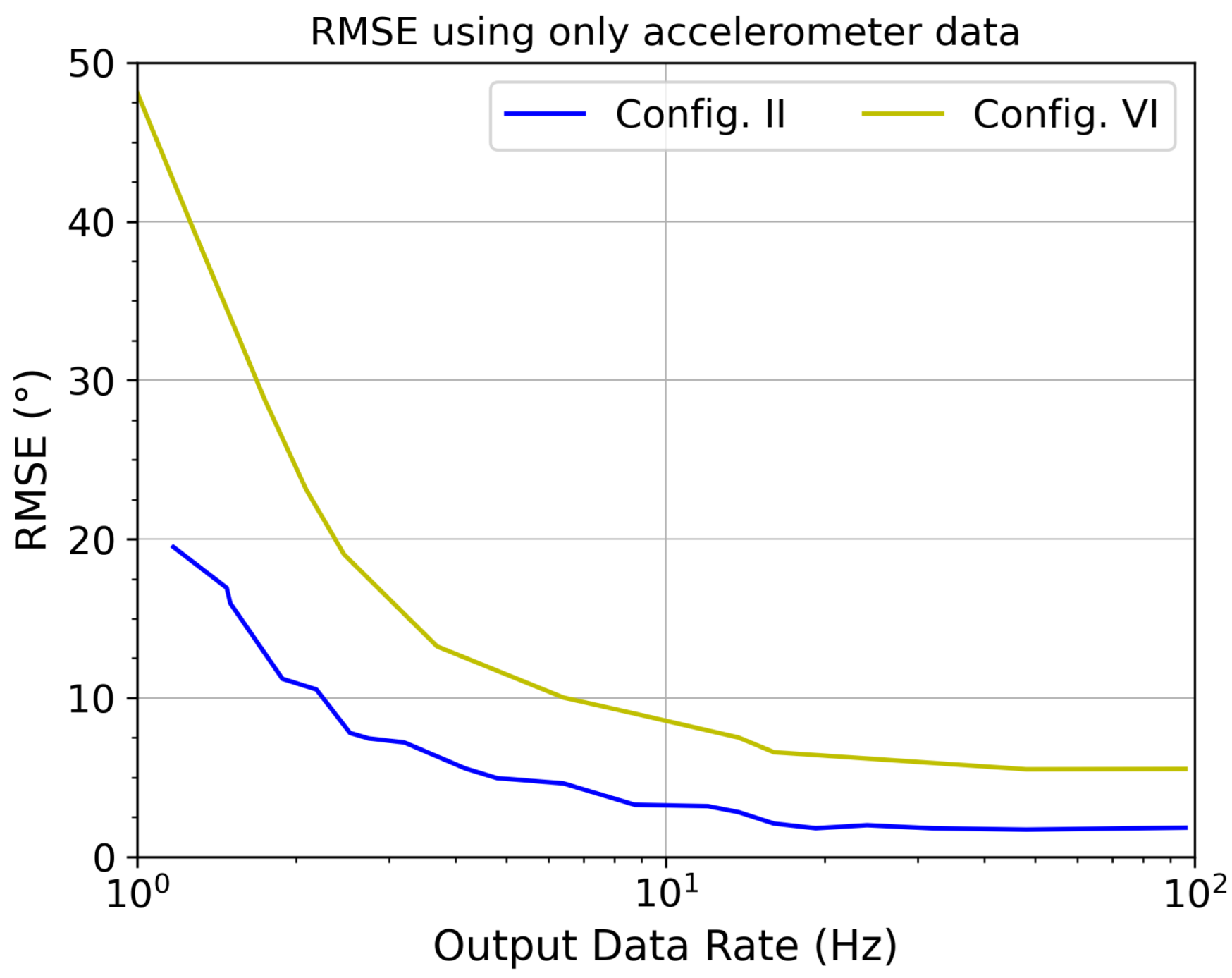
For this reason, the impact of the output data rate on the RMSE was studied considering configurations II and VI for the algorithm using only accelerometer data. As shown in Figure 8, an RMSE of only 3.2° (resp., 8.5°) is obtained for configuration II (resp., VI) with an output data rate of 10 Hz, whereas its value is 1.83° (resp. 5.52°) for an output data rate of 100 Hz. As expected, the lower the sample frequency is, the higher the RMSE is. Comparative to the angle span, this leads to a relative error of 1.78% (resp., 5.6%) at 10 Hz and 1.02% (resp., 3.68 %) at 100 Hz. Thus, a reduction in the data rate from 100 Hz to 10 Hz leads to an error only up to 1.8 times higher but to a division in the sensor’s power consumption by 4.1 considering the LSM303AGR accelerometer in normal mode and by 5.6 considering the LSM6DSL accelerometer in low-power mode. In addition, the reduction in the sensor’s data rate equally induces a division in the processor’s active power consumption by ten since there are ten times fewer angle estimates to compute. Thus, the sensor output data rate has a great impact on the power consumption. It should also be chosen according the maximum permissible RMSE to keep the sensor’s power consumption and the processor’s power consumption as low as possible.
Table 5.
Number of elementary arithmetic operations for the 5 algorithms.
Table 5.
Number of elementary arithmetic operations for the 5 algorithms.
| Arithmetic Operation | Accelero. Only 1 | Gyroscope Only 2 | Corrected Gyroscope 3 | Complem. Filter 4 | Kalman Filter 5 |
|---|---|---|---|---|---|
| + | 2 | 2 | 2 | 5 | 8 |
| − | 0 | 0 | 1 | 2 | 3 |
| × | 3 | 1 | 1 | 6 | 16 |
| / | 1 | 1 | 2 | 3 | 4 |
| √ | 1 | 0 | 0 | 1 | 1 |
| arctan | 1 | 0 | 0 | 1 | 1 |
Table 6.
The number of cycles required for each elementary arithmetic operation considering an ARM Cortex-M4 processor [31].
Table 6.
The number of cycles required for each elementary arithmetic operation considering an ARM Cortex-M4 processor [31].
| Arithmetic Operation | Number of Cycles |
|---|---|
| + | 1 |
| − | 1 |
| × | 1 |
| / | 14 |
| √ | 14 |
| arctan 1 | 25 |
1 The number of cycles required to compute the result of the arctangent function is supposed to be equal to that for the CORDIC (COordinate Rotation DIgital Computer) co-processor developed by STMicroelectronics and integrated into STM32G4 series microcontrollers based on an ARM Cortex-M4 processor [32].
Table 7.
Total number of cycles for the 5 algorithms assuming an ARM Cortex-M4 processor.
Table 7.
Total number of cycles for the 5 algorithms assuming an ARM Cortex-M4 processor.
| Algorithm | Accelero. Only | Gyroscope Only | Corrected Gyroscope | Complem. Filter | Kalman Filter |
|---|---|---|---|---|---|
| Cycles number | 58 | 17 | 32 | 94 | 122 |
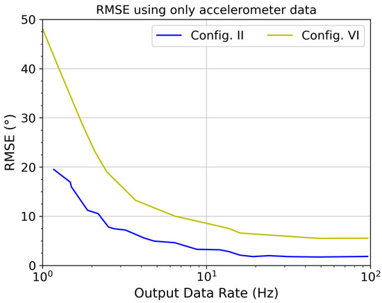
Figure 8.
The RMSE obtained for configurations II and VI with the algorithm using only accelerometer data versus the sensor’s output data rate.
4.2. The Angular Speed and the Sensor–Joint Distance
As indicated previously, the robotic arm allows us to evaluate the impact of the angular speed and the impact of the distance between the sensor and the limb joint; both can be linked to the sensor’s speed of motion. The results obtained with the relevant configurations are presented together in Table 8 (resp., Table 9) to highlight effects of the angular speed (resp., the distance between the sensor and the joint).
Table 8.
The RMSE obtained with the algorithm using only the accelerometer data according to the average angular speed during motion.
Table 9.
The RMSE obtained with the algorithm using only the accelerometer data according to the distance between the sensor and the joint.
From Table 8, it appears that the higher the angular speed is, the higher the RMSE obtained using only accelerometer data is. The use of a standalone accelerometer is also relevant only when exercises are not carried out at an excessive angular speed (it should be noted that the sensor’s speed of movement is proportional to the angular speed). However, the opposite behavior can be seen when only gyroscope data are used without correction. Nevertheless, the use of bias correction for the gyroscope allows us to approximately obtain an RMSE independent of the angular speed. The angular speed should only have an impact on the gyroscope’s drift when the motions are regular. However, the RMSE obtained with bias correction for the gyroscope remains higher than the RMSE obtained using only the accelerometer data.
Finally, according to Table 8, the longer the distance between the sensor and the joint is, the higher the RMSE obtained using only the accelerometer data is. As seen previously, the opposite behavior can be seen when only the gyroscope data are used without correction. Nevertheless, the gyroscope drift correction, again, allows for stabilization of the RMSE. These observations confirm those made previously since the sensor’s movement speed is proportional to the distance between the sensor and the joint.
4.3. Comparison with Other Works
The results obtained in this paper using only accelerometer data can be compared with other works in Table 10 for sensor data rates of 10 Hz and 100 Hz. However, only the results for configurations II and VI are reported since their angular speeds and sensor–joint distances are close to those in real rehabilitation or mobility evaluation exercises.
From Table 10, it can be seen that most papers use at least two types of sensors and that accelerometers are generally associated with gyroscopes. Nevertheless, the use of an additional magnetometer seems to be relevant since two of the three best references in terms of the RMSE both use this type of sensor [22,33].
According to Table 10, using a high number of devices does not inevitably lead to better results. Indeed, the best results were obtained using two devices. Moreover, the RMSE obtained in this paper using only one device is comparable to that obtained with a higher number of devices considering a sensor data rate of 100 Hz.
Similarly, the most complex algorithms, such as artificial neural networks (ANNs) or Extended Kalman Filter (EKF), do not necessarily lead to the best results. For instance, only one of the three best references in terms of the RMSE uses a Kalman filter [22], whereas at least one of the two others uses standard low-pass and high-pass filtering [34].
Finally, the RMSE values obtained in other work seem to follow the trend of the sensor’s data rate needing to be chosen according to the targeted precision. However, it should be noted that the third best results in terms of the RMSE were obtained using a sensor data rate of only 20 Hz [33]. Nevertheless, the results obtained in this paper using only accelerometer data and a sensor data rate of 10 Hz remain comparable to those of other works, whereas they require only one low-power accelerometer and a low number of processor cycles.
Table 10.
Comparison table with other works.
Table 10.
Comparison table with other works.
| Config. or Reference | RMSE Min/Max (°) | STD Min/Max (°) | Correlation Max/Min (%) | Sensor 1/ Algorithm 2 | Device Number | Studied Member | Angular Speed (°/s) | Angle Span (°) | Sensor Data Rate (Hz) |
|---|---|---|---|---|---|---|---|---|---|
| II/VI | 3.23/8.5 | 3.17/8.5 | - | A/LPF | 1 | Arm | 83.3 | 150 | 10 |
| II/VI | 1.83/5.52 | 1.69/5.52 | 99.9/99.6 | A/LPF | 1 | Arm | 83.3 | 150 | 100 |
| [33] | 0.87/1.37 | 0.83/1.24 | - | AM/- | 2 | Arm | - | 50 | 20 |
| [21] | 2.13 | 2.25 | 98 | AG/KF | 2 | Arm | <80 | 90 | 25 |
| [35] | 1.36/3.33 | - | 97/87 | AGM/- | 2 | Leg | - | 50 | 100 |
| [34] | 0.63/2.92 | - | - | AG/LPHP | 2 | Leg | - | 70 | 100 |
| [22] | 0.5/3.0 | - | 99/97 | AGM/KF | 2 | Leg | - | 50 | 120 |
| [36] | 2.37/4.86 | 0.78/1.97 | 99 | AG/CF | 2 | Leg | - | - | 1500 |
| [37] | 4.37/6.45 | - | - | G/EKF | 4 | Leg | - | - | 50 |
| [24] | 1.62/3.30 | - | - | AG/CF | 4 | Leg | ≈180 | 80 | 60 |
| [38] | 3.89 | - | 98 | AG/ANN | 5 | Leg | - | 60 | 100 |
| [39] | 2.2/5.1 | 0.9/2.7 | 99/67 | AG/ANN | 5 | Leg | - | - | 100 |
1 Accelerometer (A), gyroscope (G), and magnetometer (M). 2 Low-pass filter (LPF), low-pass and high-pass filters (LPHP), Kalman filter (KF), complementary filter (CF), Extended Kalman Filter (EKF), and artificial neural network (ANN).
5. Conclusions
In this paper, elbow joint angle estimation algorithms using a low-cost and low-power single inertial device for daily home-based self-rehabilitation were investigated. During the experiments, a robotic arm and a human arm were used to obtain the error interval for each tested algorithm, with the robotic arm allowing for reproducible movements and also the acquisition of reproducible results, which allowed us to verify the impact of parameters such as the sensor speed independently. The results of the experiments show that the algorithms using only accelerometer data, the complementary filter, and the Kalman filter lead to the best results, which are very close in terms of the RMSE. However, the complementary filter and the Kalman filter require a high number of computing cycles and also imply higher power consumption. Moreover, the complementary filter and the Kalman filter require an additional sensor for data fusion (such as a gyroscope, which can have a power consumption ten times higher than that of an accelerometer), which increases the power consumption of both filters. Thus, the presented algorithm using only accelerometer data should be preferred to minimize the power consumption.
Moreover, the impact of the sensor’s output data rate was investigated. It appears that the sensor’s data rate can be reduced, thereby reducing the power consumption more than the error is increased (a reduction in the data rate from 100 Hz to 10 Hz multiplied the RMSE obtained here by about 1.8 but could divide the power consumption associated with the sensor and the algorithm computation by up to 10). However, the experimental results show that the higher the sensor’s speed of motion is, the higher the error obtained with only the accelerometer data is. Nevertheless, the algorithm that uses only accelerometer data stays well suited to rehabilitation exercises or mobility evaluations since the sensor’s movement speed is also moderate.
Thus, at a time with increasing algorithmic complexity (sensor fusion, neural networks, etc.) and associated environmental costs, these results show that simpler and less expensive solutions can be accurate enough to contribute to healthcare improvements. To go further, a miniature device containing only a BLE module, an accelerometer, and a battery needs to be designed. By using a state-of-the-art BLE module and accelerometer in terms of their power consumption, the energy consumption, and therefore the autonomy of the designed device, could then be estimated and optimized. Then, clinical trials will need to be conducted on a significant number of patients to, on the one hand, validate the accuracy of the algorithm and, on the other hand, verify the ease of use of the device.
Author Contributions
Conceptualization: M.F. and R.V. Methodology: M.F. and R.V. Software: M.F. and R.V. Validation: G.R. and E.W. Formal analysis: M.F. and R.V. Investigation: M.F., R.V., G.R. and E.W. Resources: G.R., E.W. and E.K. Data curation: R.V. Writing—original draft preparation: M.F. and R.V. Writing—review and editing: M.F., R.V., G.R., E.W. and E.K. Visualization: M.F. and R.V. Supervision: R.V. and E.K. All authors have read and agreed to the published version of the manuscript.
Funding
This research received no external funding.
Informed Consent Statement
Informed consent was obtained from all subjects involved in the study.
Data Availability Statement
The original contributions presented in this study are included in the article. Further inquiries can be directed to the corresponding author.
Conflicts of Interest
The authors declare no conflicts of interest.
References
- OECD. Health at a Glance 2023: OECD Indicators; OECD Publishing: Paris, France, 2023. [Google Scholar] [CrossRef]
- Lee, S.I.; Adans-Dester, C.P.; O’Brien, A.T.; Vergara-Diaz, G.P.; Black-Schaffer, R.; Zafonte, R.; Dy, J.G.; Bonato, P. Predicting and Monitoring Upper-Limb Rehabilitation Outcomes Using Clinical and Wearable Sensor Data in Brain Injury Survivors. IEEE Trans. Biomed. Eng. 2021, 68, 1871–1881. [Google Scholar] [CrossRef]
- Benjelloun, Z.; Vauche, R.; Rahajandraibe, W.; Bouchakour, R. Design of an energy detector for heartbeat localization in ECG signals. In Proceedings of the 2016 IEEE International Conference on Electronics, Circuits and Systems (ICECS), Monte Carlo, Monaco, 11–14 December 2016; pp. 73–76. [Google Scholar] [CrossRef]
- Ram, M.R.; Madhav, K.V.; Krishna, E.H.; Komalla, N.R.; Reddy, K.A. A Novel Approach for Motion Artifact Reduction in PPG Signals Based on AS-LMS Adaptive Filter. IEEE Trans. Instrum. Meas. 2012, 61, 1445–1457. [Google Scholar] [CrossRef]
- Ihlen, E.; van Schooten, K.; Bruijn, S.; van Dieën, J.; Vereijken, B.; Helbostad, J.; Pijnappels, M. Improved Prediction of Falls in Community-Dwelling Older Adults Through Phase-Dependent Entropy of Daily-Life Walking. Front. Aging Neurosci. 2018, 10, 44. [Google Scholar] [CrossRef]
- Siddharth, P.D.; Deshpande, S. Embedded system design for real-time interaction with Smart Wheelchair. In Proceedings of the 2016 Symposium on Colossal Data Analysis and Networking (CDAN), Indore, India, 18–19 March 2016; pp. 1–4. [Google Scholar] [CrossRef]
- Joukov, V.; Karg, M.; Kulic, D. Online tracking of the lower body joint angles using IMUs for gait rehabilitation. In Proceedings of the 2014 36th Annual International Conference of the IEEE Engineering in Medicine and Biology Society, Chicago, IL, USA, 26–30 August 2014; pp. 2310–2313. [Google Scholar] [CrossRef]
- Madgwick, S.O.H.; Harrison, A.J.L.; Vaidyanathan, R. Estimation of IMU and MARG orientation using a gradient descent algorithm. In Proceedings of the 2011 IEEE International Conference on Rehabilitation Robotics, Zurich, Switzerland, 29 June–1 July 2011; pp. 1–7. [Google Scholar] [CrossRef]
- Mihelj, M. Inverse Kinematics of Human Arm Based on Multisensor Data Integration. J. Intell. Robot. Syst. 2006, 47, 139–153. [Google Scholar] [CrossRef]
- Lee, G.X.; Low, K.S. A Factorized Quaternion Approach to Determine the Arm Motions Using Triaxial Accelerometers With Anatomical and Sensor Constraints. IEEE Trans. Instrum. Meas. 2012, 61, 1793–1802. [Google Scholar] [CrossRef]
- Du, G.; Ding, Z.; Guo, H.; Song, M.; Jiang, F. Estimation of Lower Limb Joint Angles Using sEMG Signals and RGB-D Camera. Bioengineering 2024, 11, 1026. [Google Scholar] [CrossRef]
- Li, H.B.; Guan, X.R.; Li, Z.; Zou, K.F.; He, L. Estimation of Knee Joint Angle from Surface EMG Using Multiple Kernels Relevance Vector Regression. Sensors 2023, 23, 4934. [Google Scholar] [CrossRef] [PubMed]
- Tang, Z.; Yu, H.; Cang, S. Impact of Load Variation on Joint Angle Estimation From Surface EMG Signals. IEEE Trans. Neural Syst. Rehabil. Eng. 2016, 24, 1342–1350. [Google Scholar] [CrossRef]
- Putro, N.A.S.; Avian, C.; Prakosa, S.W.; Mahali, M.I.; Leu, J.S. Estimating finger joint angles by surface EMG signal using feature extraction and transformer-based deep learning model. Biomed. Signal Process. Control 2024, 87, 105447. [Google Scholar] [CrossRef]
- Taunyazov, T.; Omarali, B.; Shintemirov, A. A novel low-cost 4-DOF wireless human arm motion tracker. In Proceedings of the 2016 6th IEEE International Conference on Biomedical Robotics and Biomechatronics (BioRob), Singapore, 26–29 June 2016; pp. 157–162. [Google Scholar] [CrossRef]
- Schepers, M.; Giuberti, M.; Bellusci, G. Xsens MVN: Consistent Tracking of Human Motion Using Inertial Sensing; Xsens: Enschede, The Netherlands, 2018. [Google Scholar] [CrossRef]
- Robert-Lachaine, X.; Mecheri, H.; Larue, C.; Plamondon, A. Validation of inertial measurement units with an optoelectronic system for whole-body motion analysis. Med. Biol. Eng. Comput. 2016, 55, 609–619. [Google Scholar] [CrossRef]
- Bouvier, B.; Duprey, S.; Claudon, L.; Dumas, R.; Savescu, A. Upper Limb Kinematics Using Inertial and Magnetic Sensors: Comparison of Sensor-to-Segment Calibrations. Sensors 2015, 15, 18813–18833. [Google Scholar] [CrossRef]
- Müller, P.; Bégin, M.A.; Schauer, T.; Seel, T. Alignment-Free, Self-Calibrating Elbow Angles Measurement Using Inertial Sensors. IEEE J. Biomed. Health Inform. 2017, 21, 312–319. [Google Scholar] [CrossRef]
- Meng, D.; Vejarano, G. Development of a wireless sensor network for the measurement of human joint angles. In Proceedings of the 2013 International Conference on Connected Vehicles and Expo (ICCVE), Las Vegas, NV, USA, 2–6 December 2013; pp. 356–361. [Google Scholar] [CrossRef]
- Zhou, H.; Hu, H. Reducing Drifts in the Inertial Measurements of Wrist and Elbow Positions. IEEE Trans. Instrum. Meas. 2010, 59, 575–585. [Google Scholar] [CrossRef]
- Mayorca, D.; Caicedo-Eraso, J.C.; Peluffo-Ordóñez, D. Knee Joint Angle Measuring Portable Embedded System based on Inertial Measurement Units for Gait Analysis. Int. J. Adv. Sci. Eng. Inf. Technol. 2020, 10, 430–437. [Google Scholar] [CrossRef]
- Zhang, X.; Xiao, W. A Fuzzy Tuned and Second Estimator of the Optimal Quaternion Complementary Filter for Human Motion Measurement with Inertial and Magnetic Sensors. Sensors 2018, 18, 3517. [Google Scholar] [CrossRef] [PubMed]
- Seel, T.; Raisch, J.; Schauer, T. IMU-Based Joint Angle Measurement for Gait Analysis. Sensors 2014, 14, 6891–6909. [Google Scholar] [CrossRef]
- Fisher, C.J. AN-1057: Using an Accelerometer for Inclination Sensing; Analog Devices: Wilmington, MA, USA, 2010; Revision 0. [Google Scholar]
- Thrun, S.; Burgard, W.; Fox, D. Probabilistic Robotics; MIT Press: Cambridge, MA, USA, 2005. [Google Scholar]
- Zitouni, W.; Vauche, R.; Aziza, H.; Ayache, L.; Makdissi, A. Cortex-M0+-based Pacemaker: CMOS Technologies Benchmark to Achieve Ultra-Low Power Operations. In Proceedings of the 2023 IEEE International Conference on Design, Test and Technology of Integrated Systems (DTTIS), Gammarth, Tunisia, 1–4 November 2023; pp. 1–5. [Google Scholar] [CrossRef]
- Zitouni, W.; Vauche, R.; Aziza, H.; Ayache, L.; Makdissi, A. Power Consumption Reduction in Integrated Pacemakers: Design Strategies for Cortex-M0+ Processors. In Proceedings of the 2024 IEEE International Conference on Design, Test and Technology of Integrated Systems (DTTIS), Aix-En-Provence, France, 14–16 October 2024; pp. 1–7. [Google Scholar] [CrossRef]
- STMicroelectronics. LSM6DSL: iNEMO Inertial Module: Always-on 3D Accelerometer and 3D Gyroscope; STMicroelectronics: Plan-les-Ouates, Switzerland, 2010; Revision 7. [Google Scholar]
- STMicroelectronics. LSM303AGR: Ultra-Compact High-Performance eCompass Module: Ultra-Low-Power 3D Accelerometer and 3D Magnetometer; STMicroelectronics: Plan-les-Ouates, Switzerland, 2022; Revision 11. [Google Scholar]
- ARM. Cortex-M4: Technical Reference Manual; ARM: Cambridge, UK, 2010; Revision r0p0. [Google Scholar]
- STMicroelectronics. AN5325: How to Use the CORDIC to Perform Mathematical Functions on STM32 MCUs; STMicroelectronics: Plan-les-Ouates, Switzerland, 2024; Revision 6. [Google Scholar]
- Meng, D.; Shoepe, T.; Vejarano, G. Accuracy Improvement on the Measurement of Human-Joint Angles. IEEE J. Biomed. Health Inform. 2016, 20, 498–507. [Google Scholar] [CrossRef]
- Wang, S.; Cai, Y.; Hase, K.; Uchida, K.; Kondo, D.; Saitou, T.; Ota, S. Estimation of knee joint angle during gait cycle using inertial measurement unit sensors: A method of sensor-to-clinical bone calibration on the lower limb skeletal model. J. Biomech. Sci. Eng. 2022, 17, 21-00196. [Google Scholar] [CrossRef]
- Kun, L.; Inoue, Y.; Shibata, K.; Enguo, C. Ambulatory Estimation of Knee-Joint Kinematics in Anatomical Coordinate System Using Accelerometers and Magnetometers. IEEE Trans. Biomed. Eng. 2011, 58, 435–442. [Google Scholar] [CrossRef]
- Feldhege, F.; Mau-Moeller, A.; Lindner, T.; Hein, A.; Markschies, A.; Zettl, U.K.; Bader, R. Accuracy of a Custom Physical Activity and Knee Angle Measurement Sensor System for Patients with Neuromuscular Disorders and Gait Abnormalities. Sensors 2015, 15, 10734–10752. [Google Scholar] [CrossRef] [PubMed]
- Allseits, E.; Kim, K.J.; Bennett, C.; Gailey, R.; Gaunaurd, I.; Agrawal, V. A Novel Method for Estimating Knee Angle Using Two Leg-Mounted Gyroscopes for Continuous Monitoring with Mobile Health Devices. Sensors 2018, 18, 2759. [Google Scholar] [CrossRef] [PubMed]
- Liang, F.Y.; Gao, F.; Liao, W.H. Synergy-based knee angle estimation using kinematics of thigh. Gait Posture 2021, 89, 25–30. [Google Scholar] [CrossRef] [PubMed]
- Hernandez, V.; Dadkhah, D.; Babakeshizadeh, V.; Kulić, D. Lower body kinematics estimation from wearable sensors for walking and running: A deep learning approach. Gait Posture 2021, 83, 185–193. [Google Scholar] [CrossRef]


Disclaimer/Publisher’s Note: The statements, opinions and data contained in all publications are solely those of the individual author(s) and contributor(s) and not of MDPI and/or the editor(s). MDPI and/or the editor(s) disclaim responsibility for any injury to people or property resulting from any ideas, methods, instructions or products referred to in the content. |
© 2025 by the authors. Licensee MDPI, Basel, Switzerland. This article is an open access article distributed under the terms and conditions of the Creative Commons Attribution (CC BY) license (https://creativecommons.org/licenses/by/4.0/).