


Self-Parameterized Chaotic Map for Low-Cost Robust Chaos


Abstract
:1. Introduction
- We present the idea of self-parameterization in more detail.
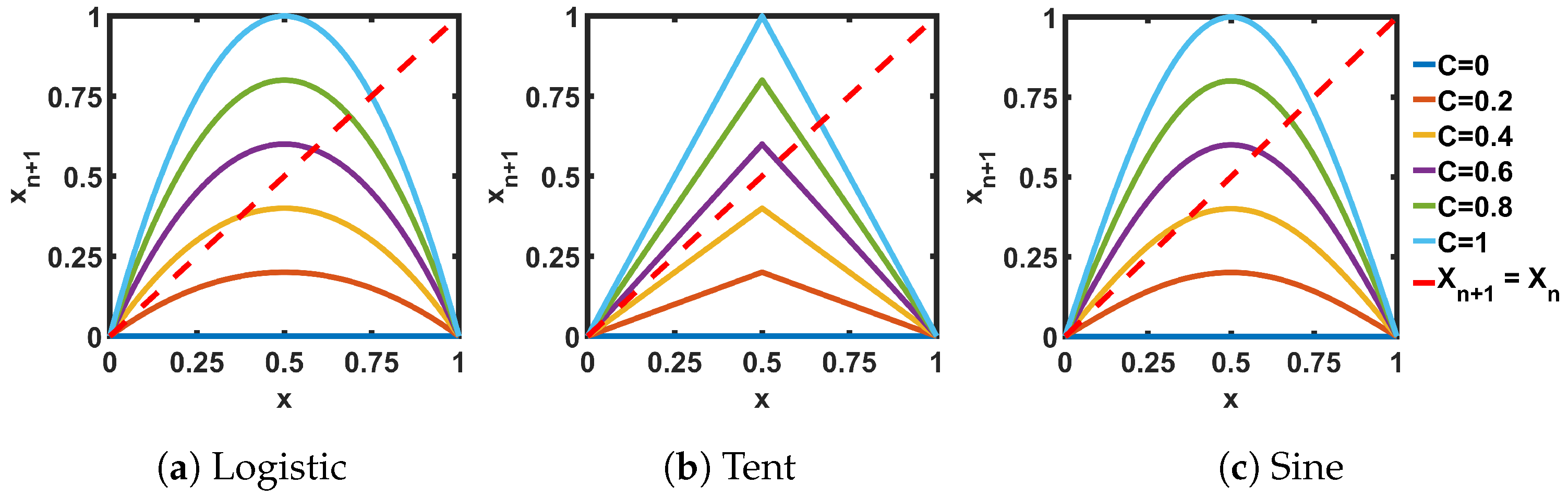
- At first, similar to the conference paper, the scheme is demonstrated in the case of three ideal mathematical maps: Logistic, Sine, and Tent maps.
- A general design methodology, in the light of stability analysis, was added to this paper.
- Similar to the conference paper, we present a design for a digitized SPM that can be implemented in FPGA.
- Then, we show the hardware-efficient CMOS-based designs for the analog implementation of SPM. In this paper, we present three different topologies of maps, and introduce the corresponding low transistor-count transformation circuits.
- The chaotic performance of the proposed designs was analyzed with different entropy metrics, along with one additional entropy metric, in this paper.
- We added an application of the proposed scheme in this paper. The application was demonstrated in a random number generator design. The cryptographic applicability of the random number generator was verified with an established statistical tool.
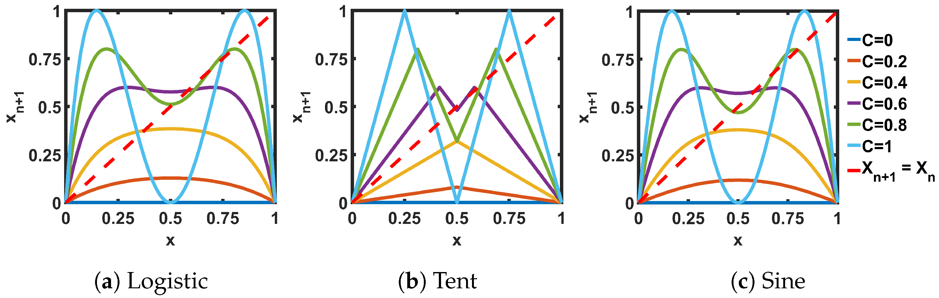
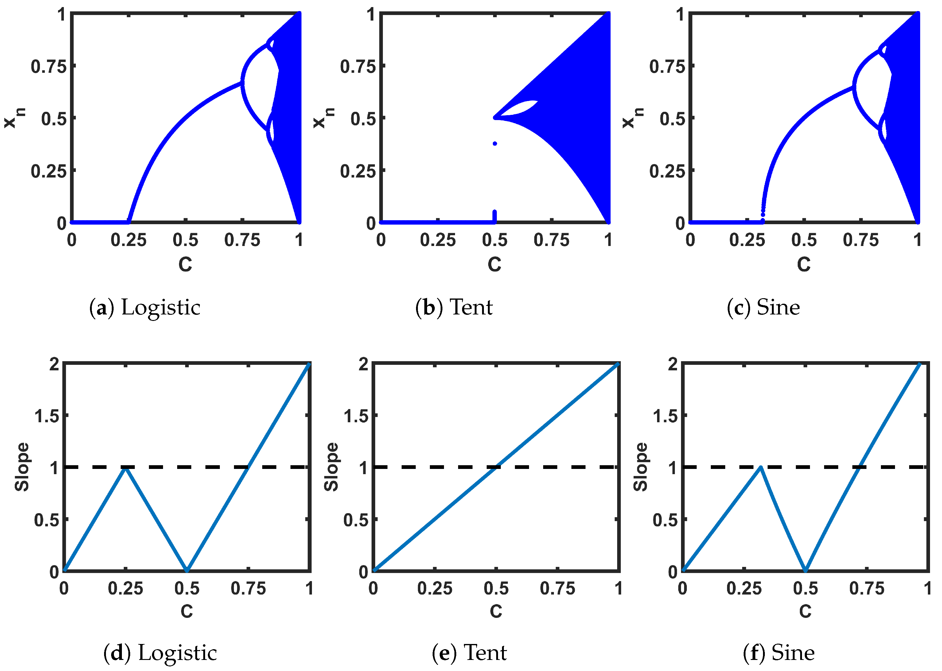
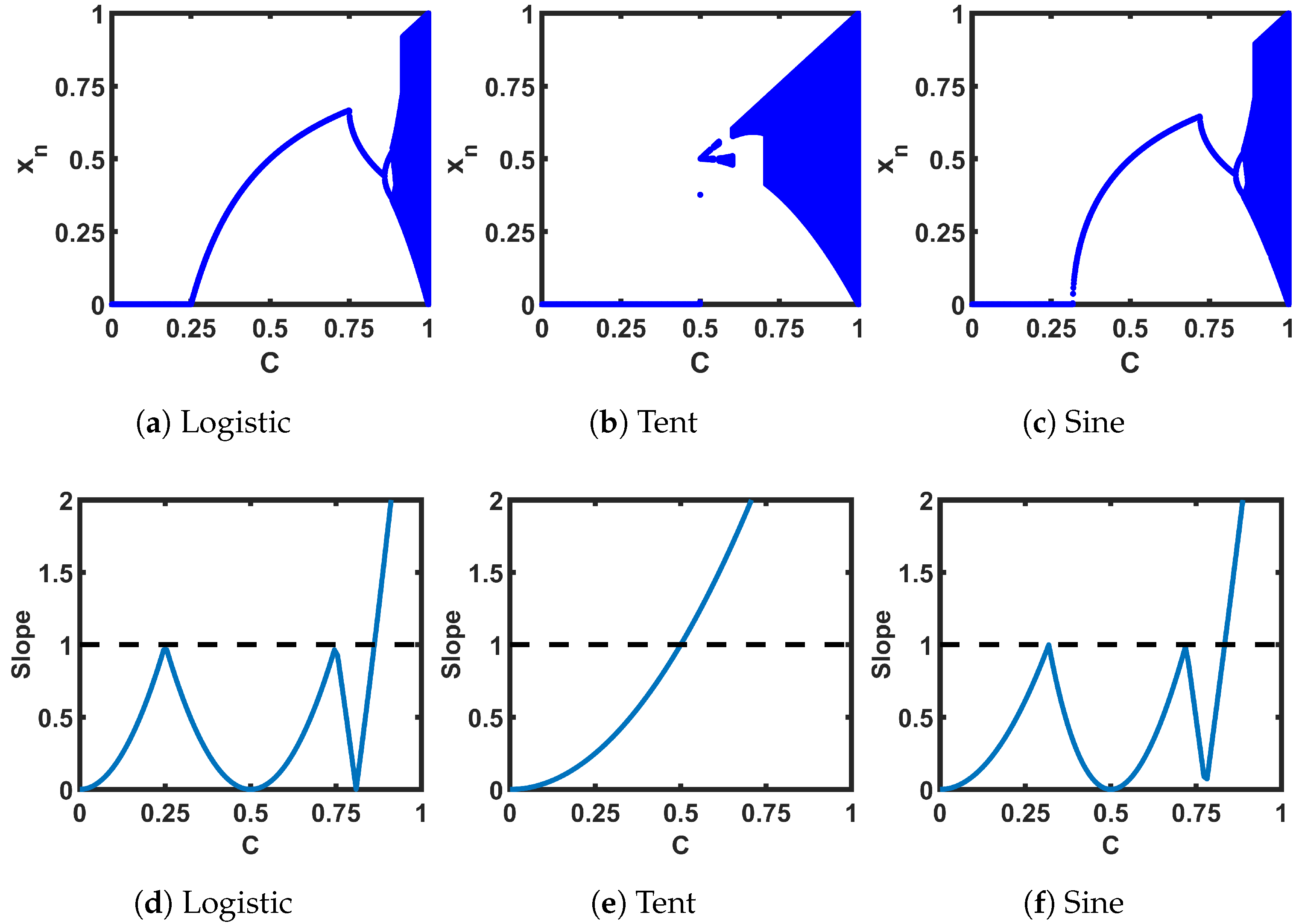
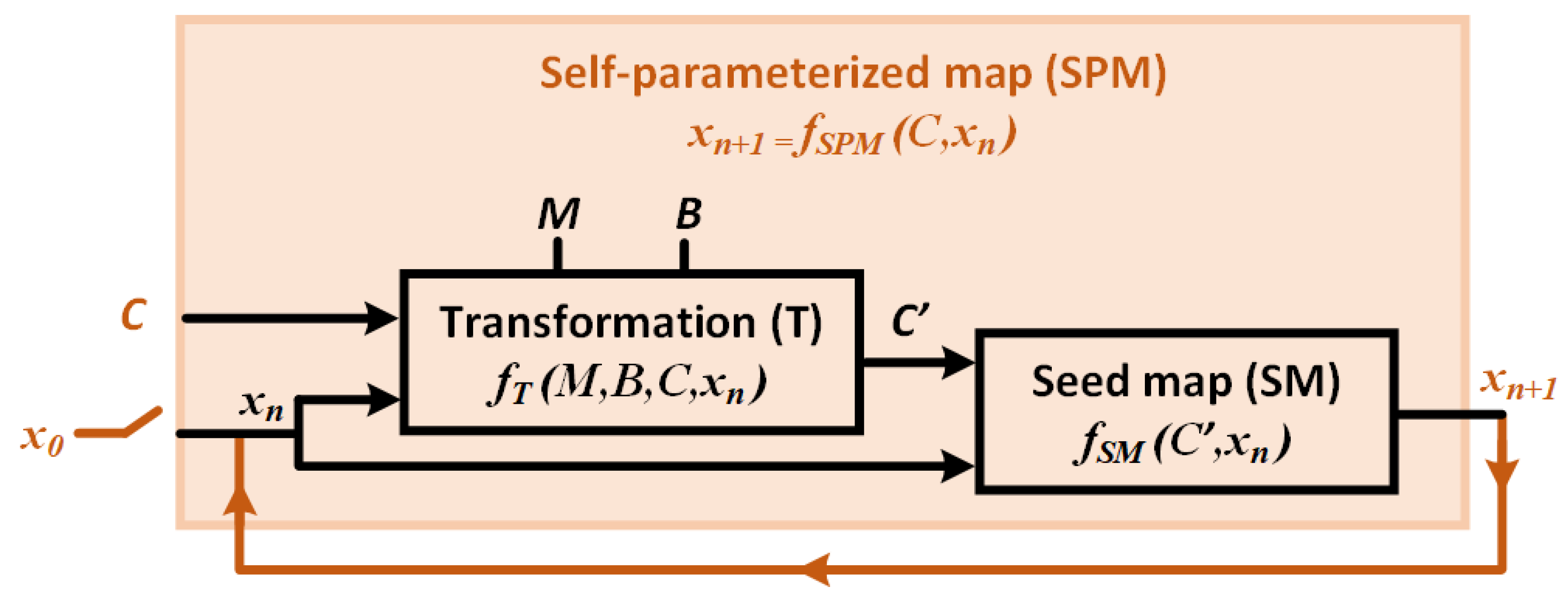
2. Proposed Scheme
3. Analytical Function-Based Maps
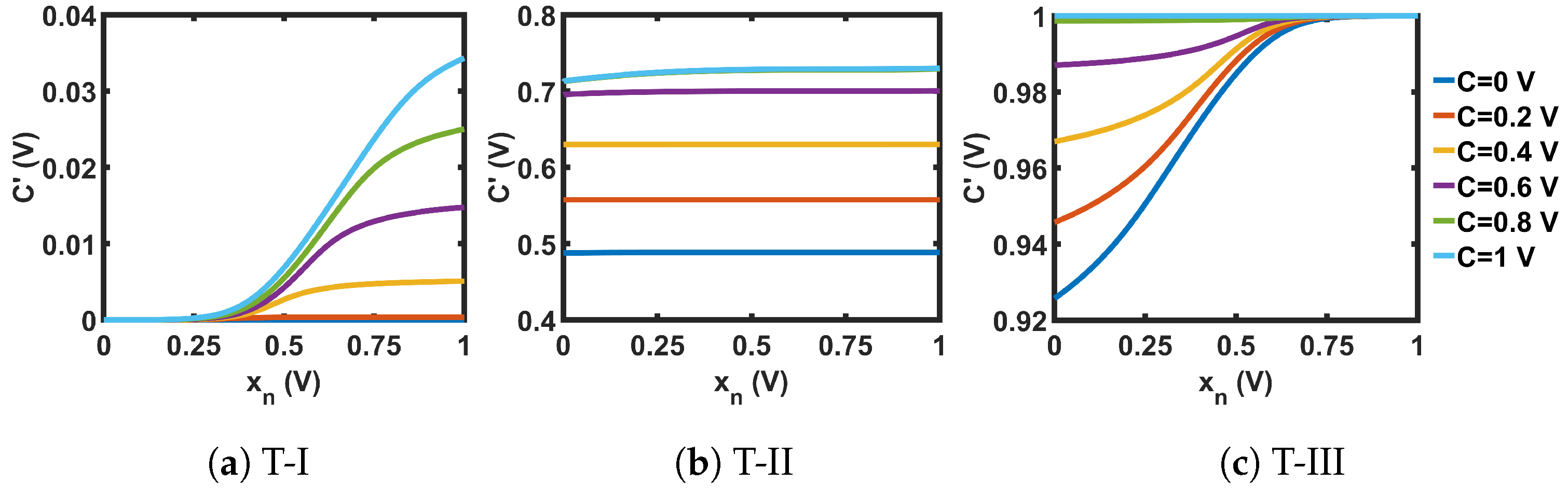
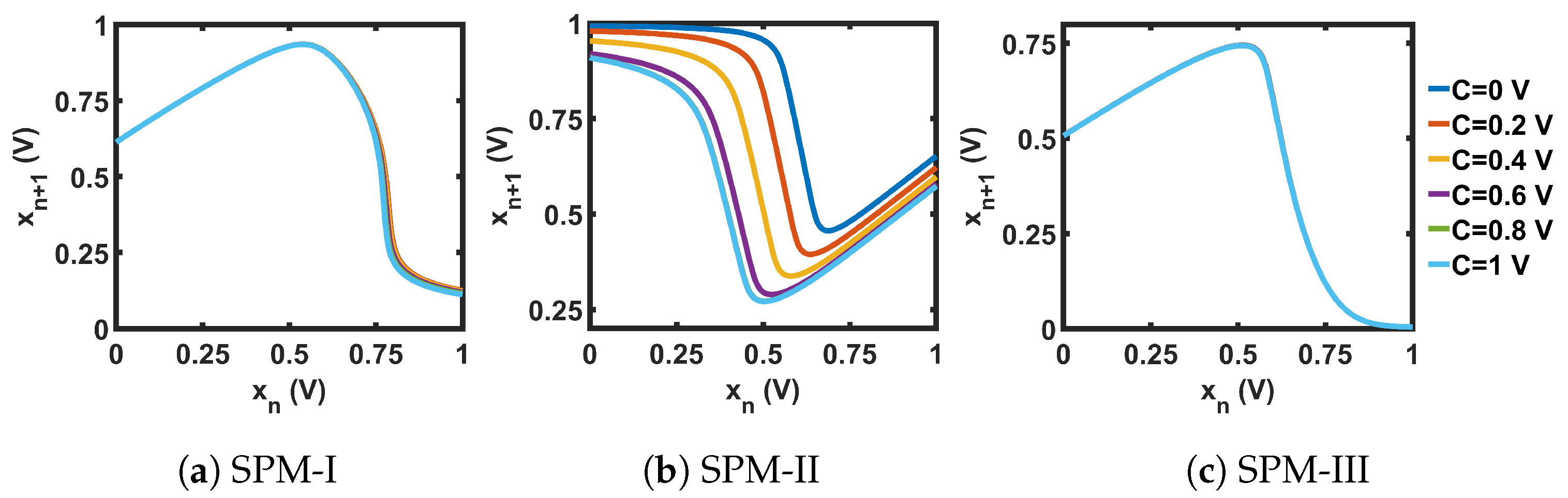
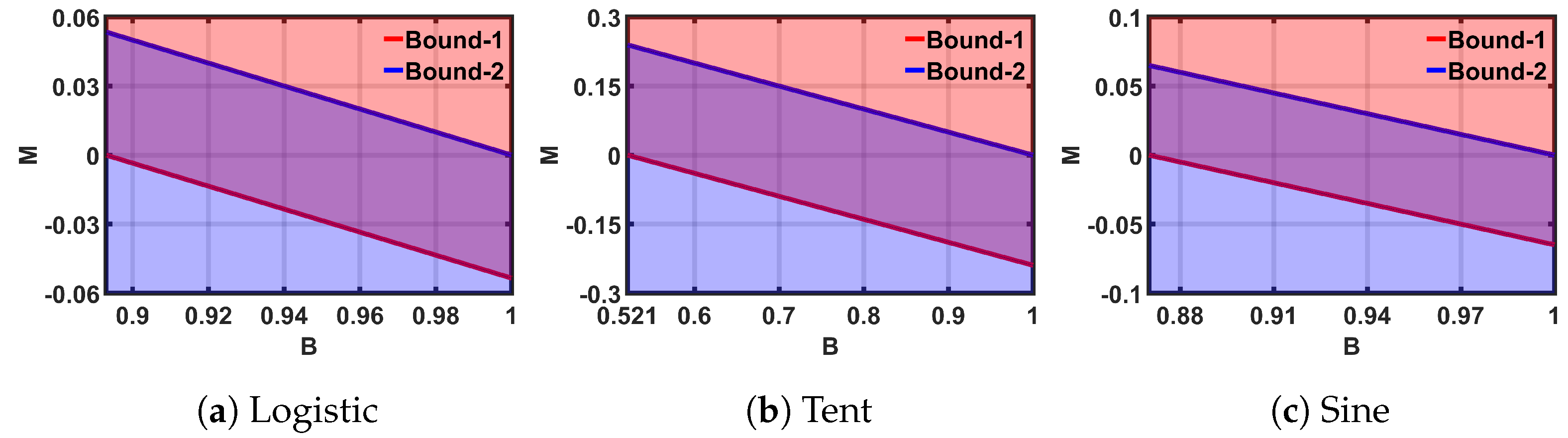
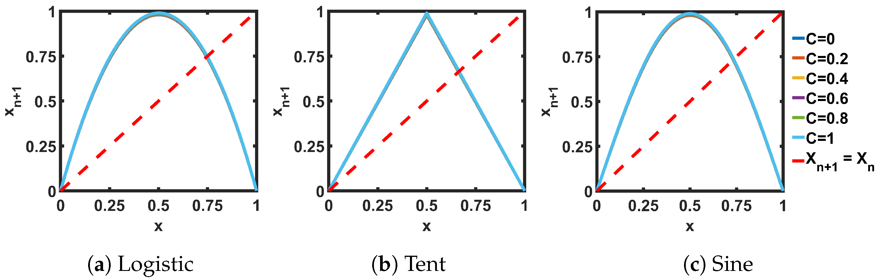
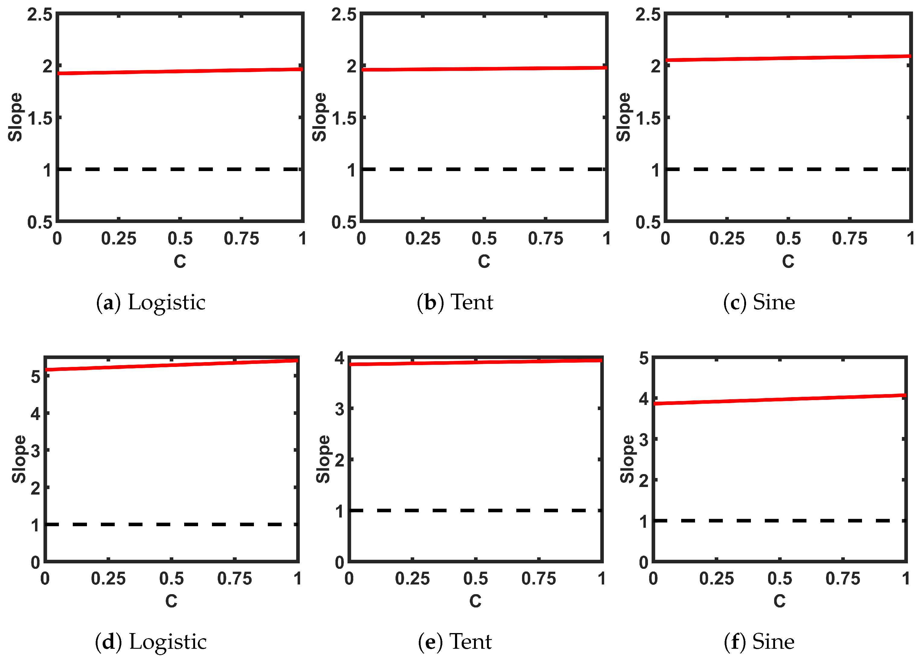
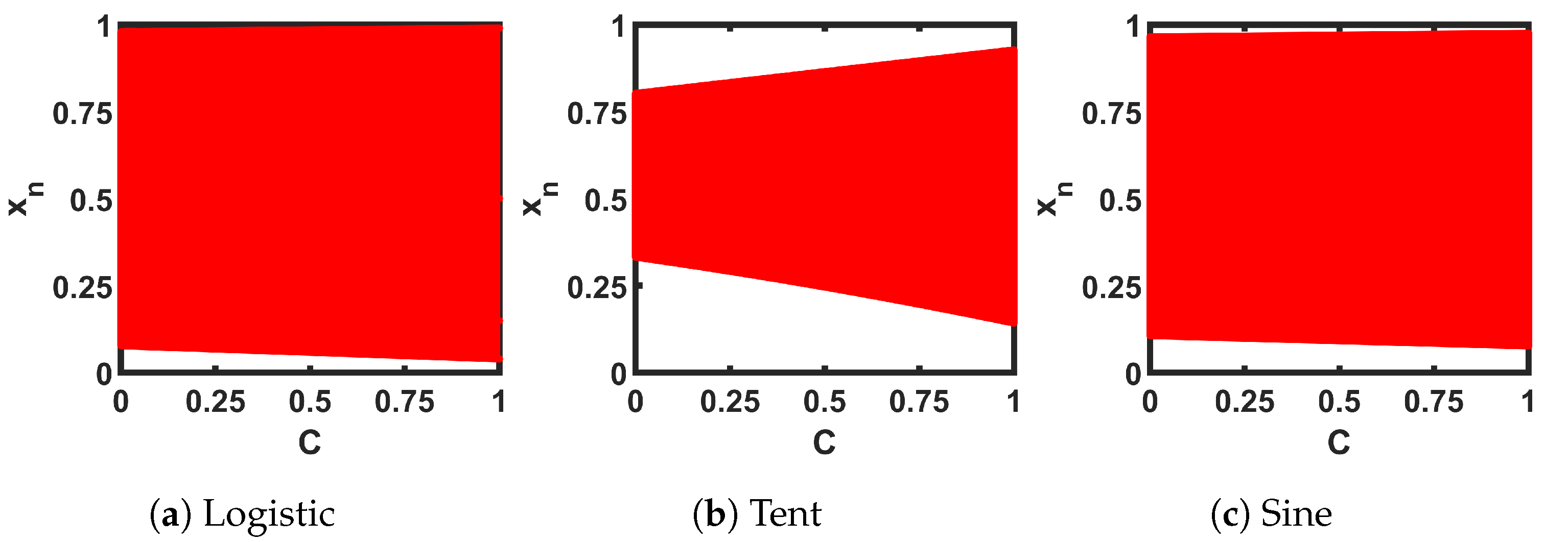
3.1. Design Methodology
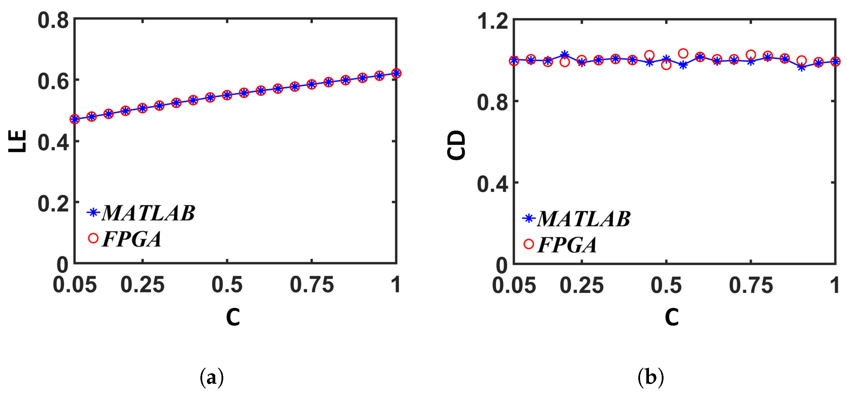
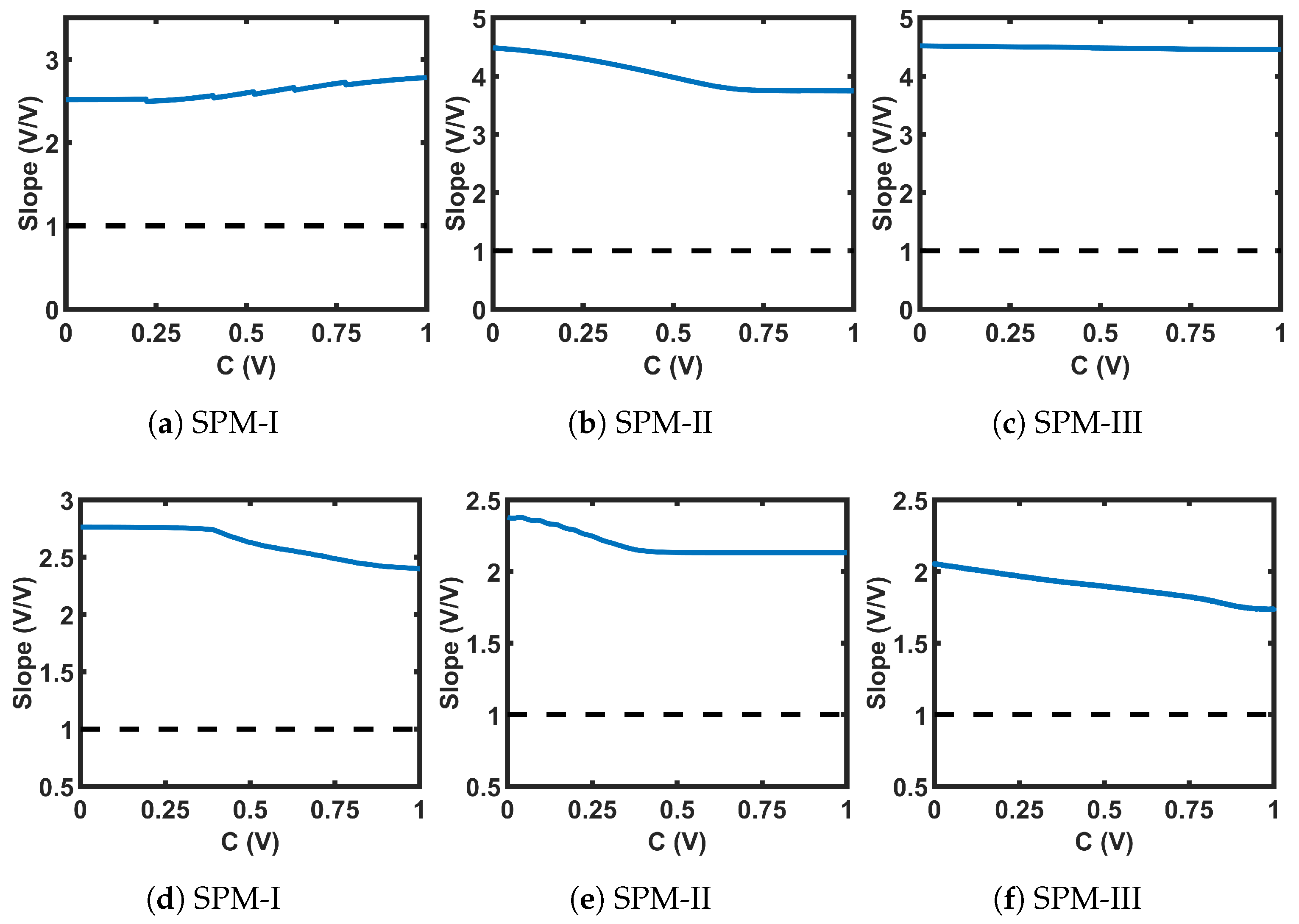
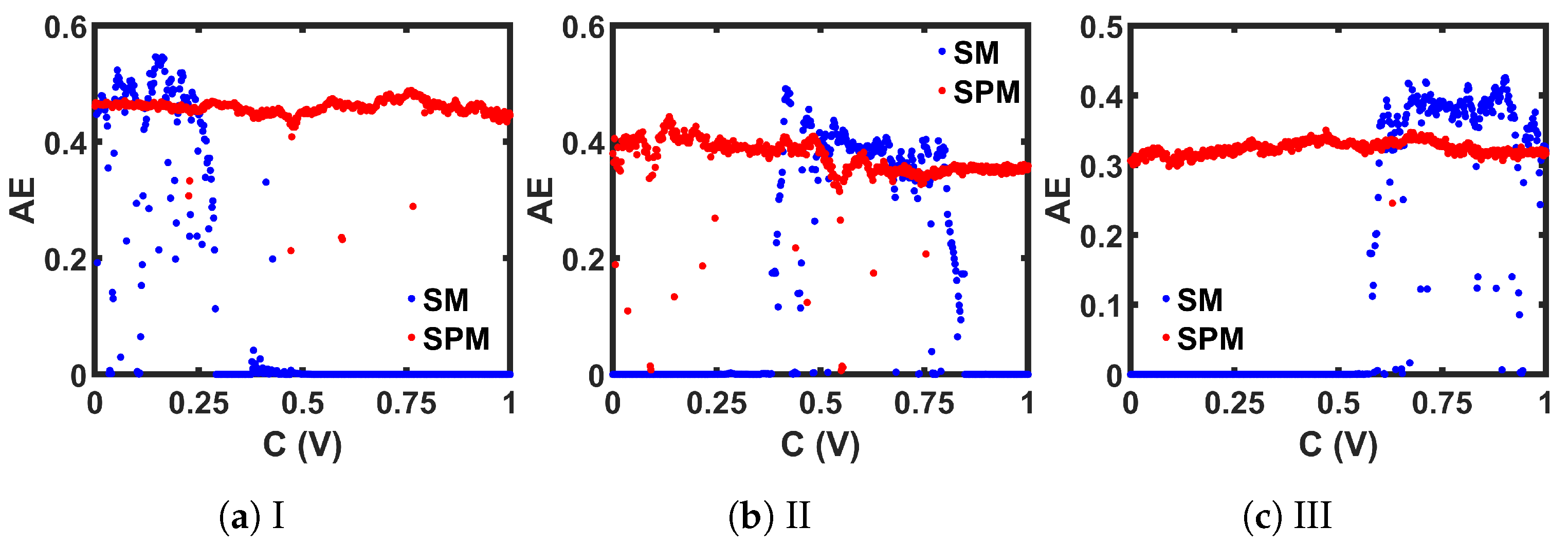
3.2. Chaotic Performance Evaluation
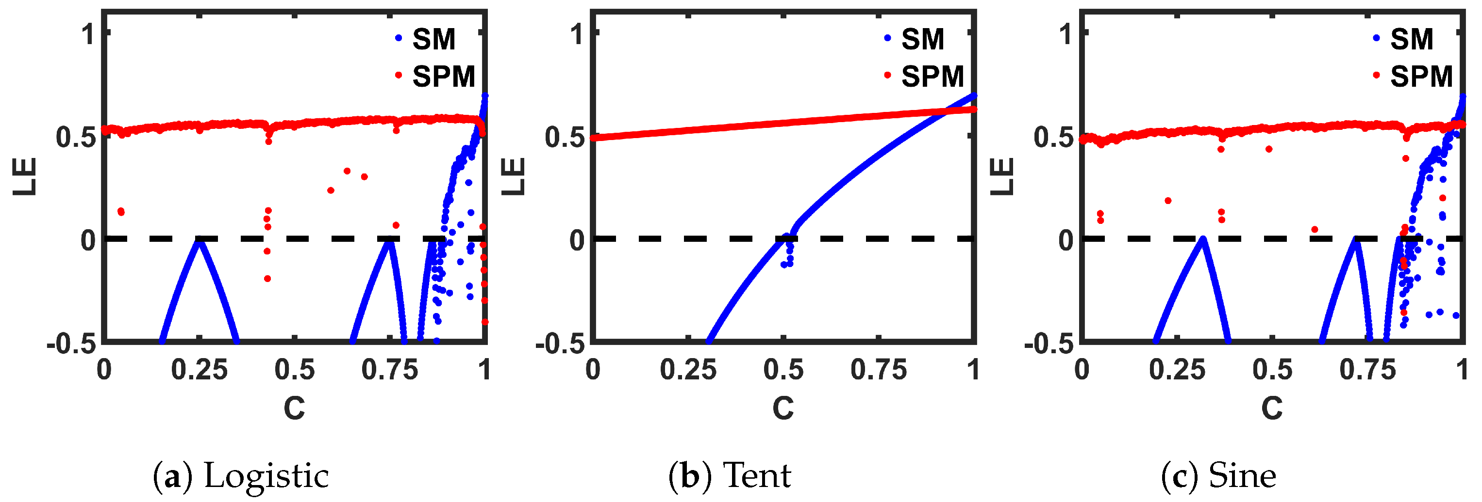
3.2.1. The Lyapunov Exponent
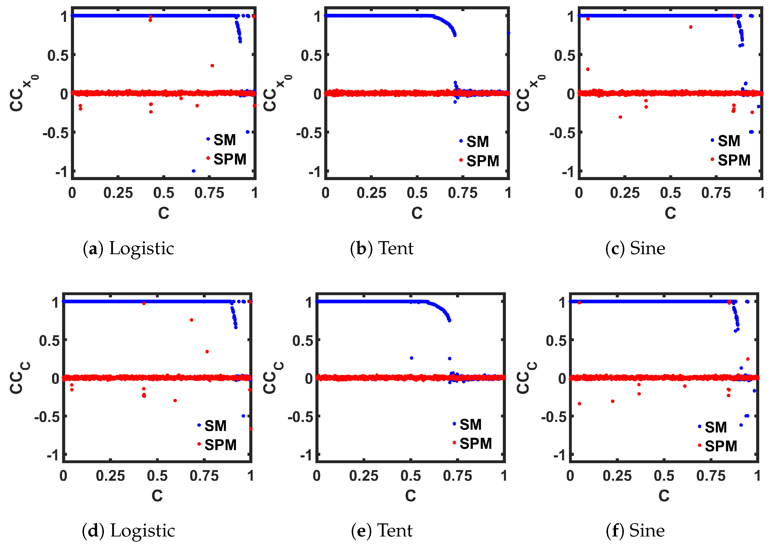
3.2.2. Correlation Coefficient
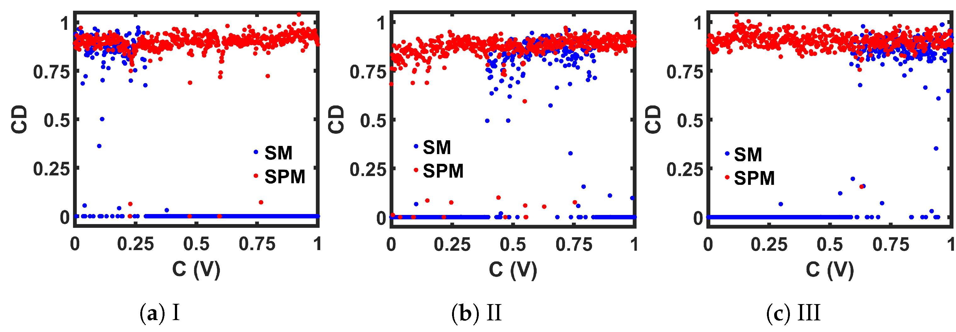
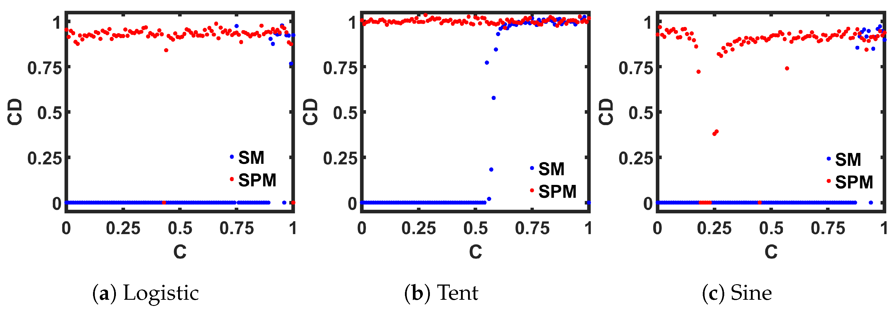
3.2.3. Correlation Dimension
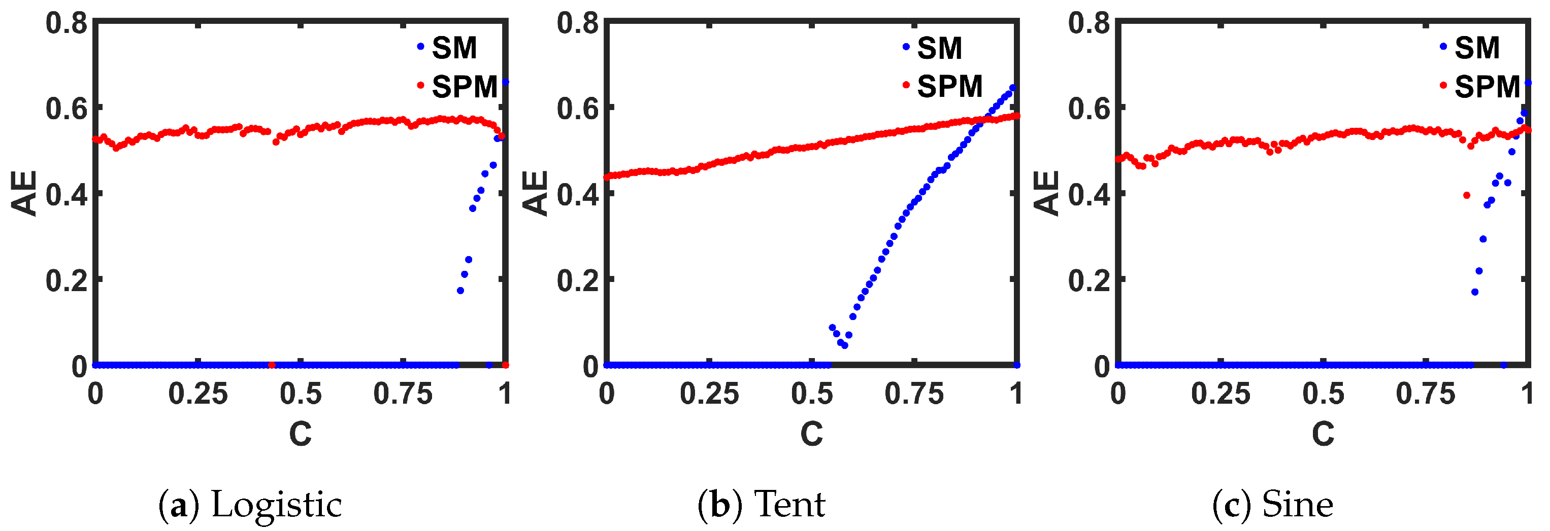
3.3. Approximate Entropy
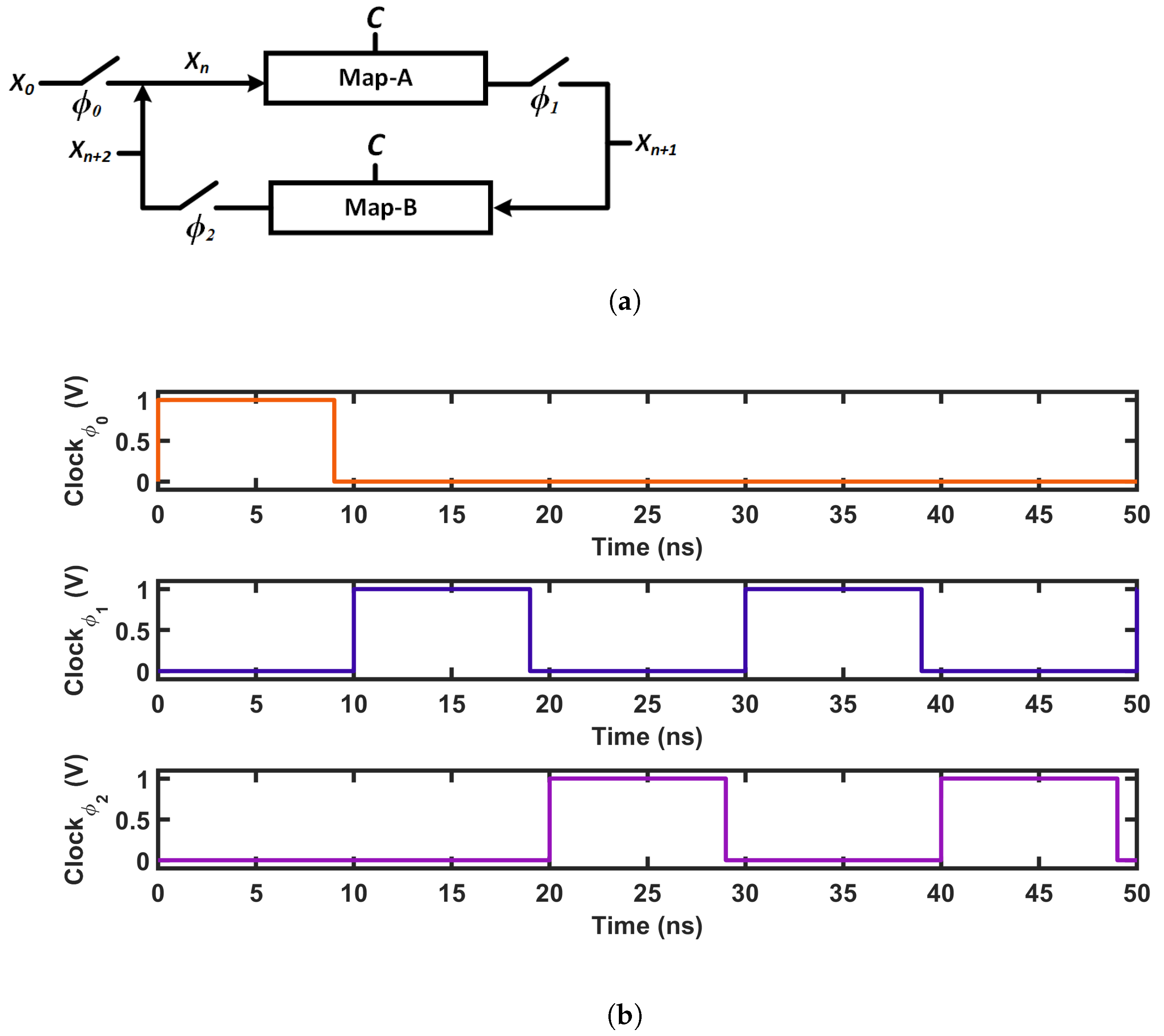
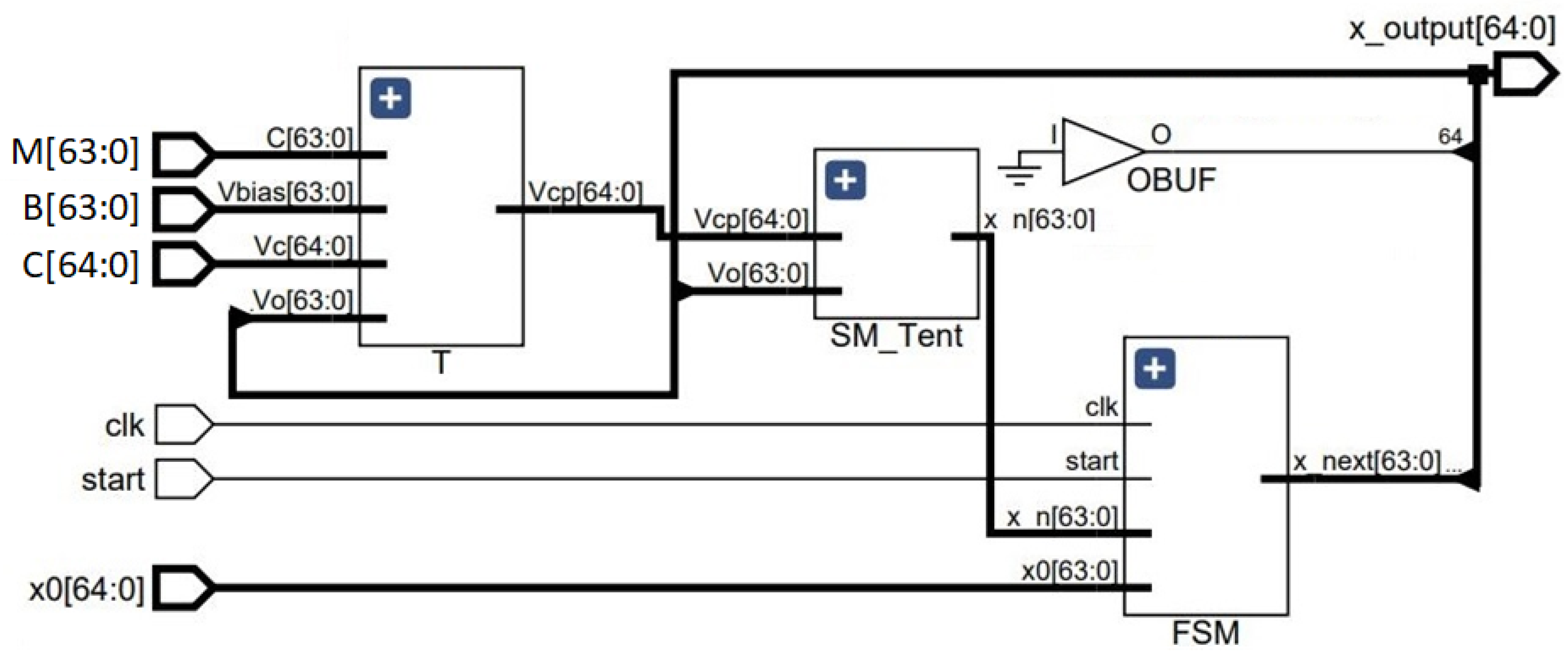
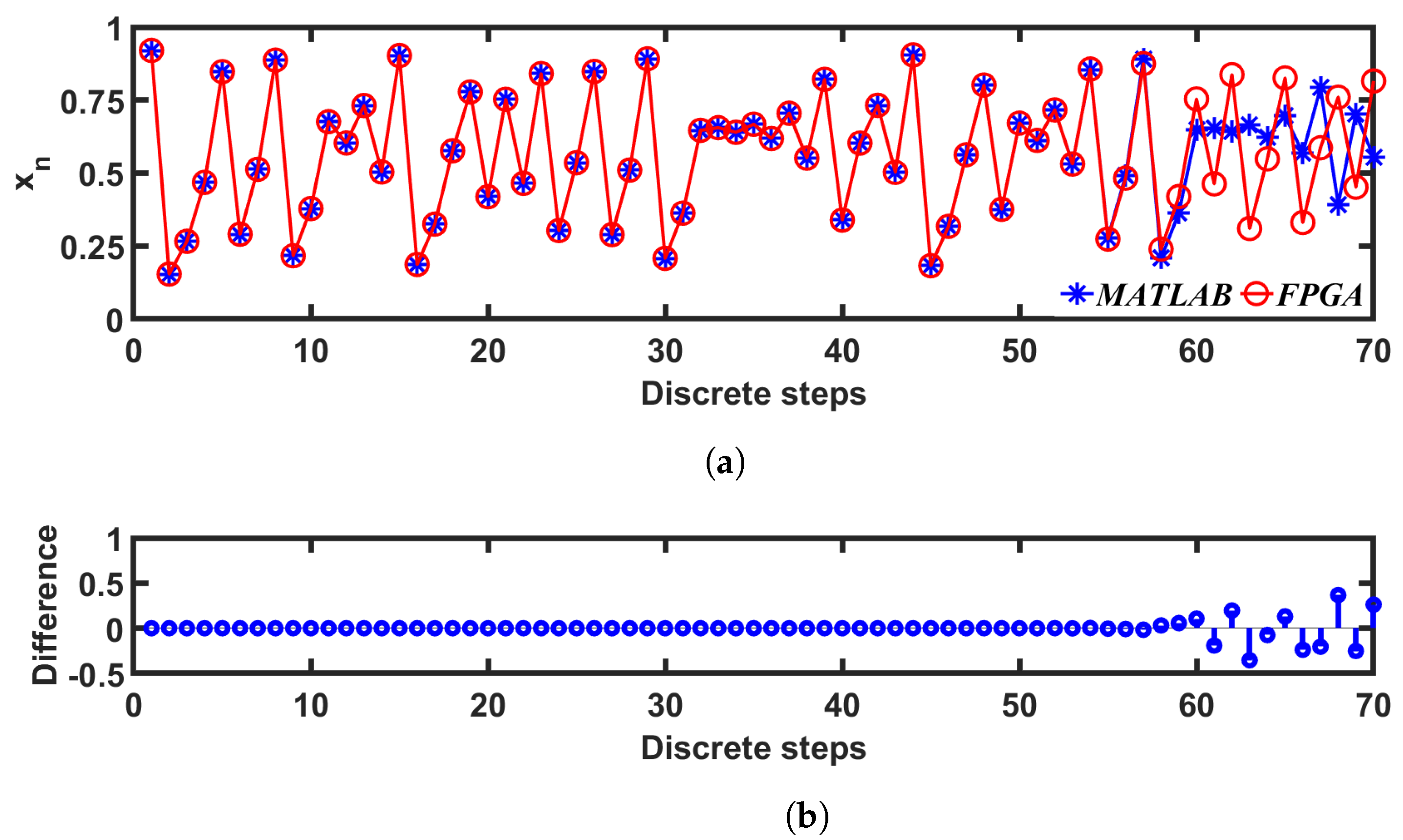
4. Design for FPGA Implementation
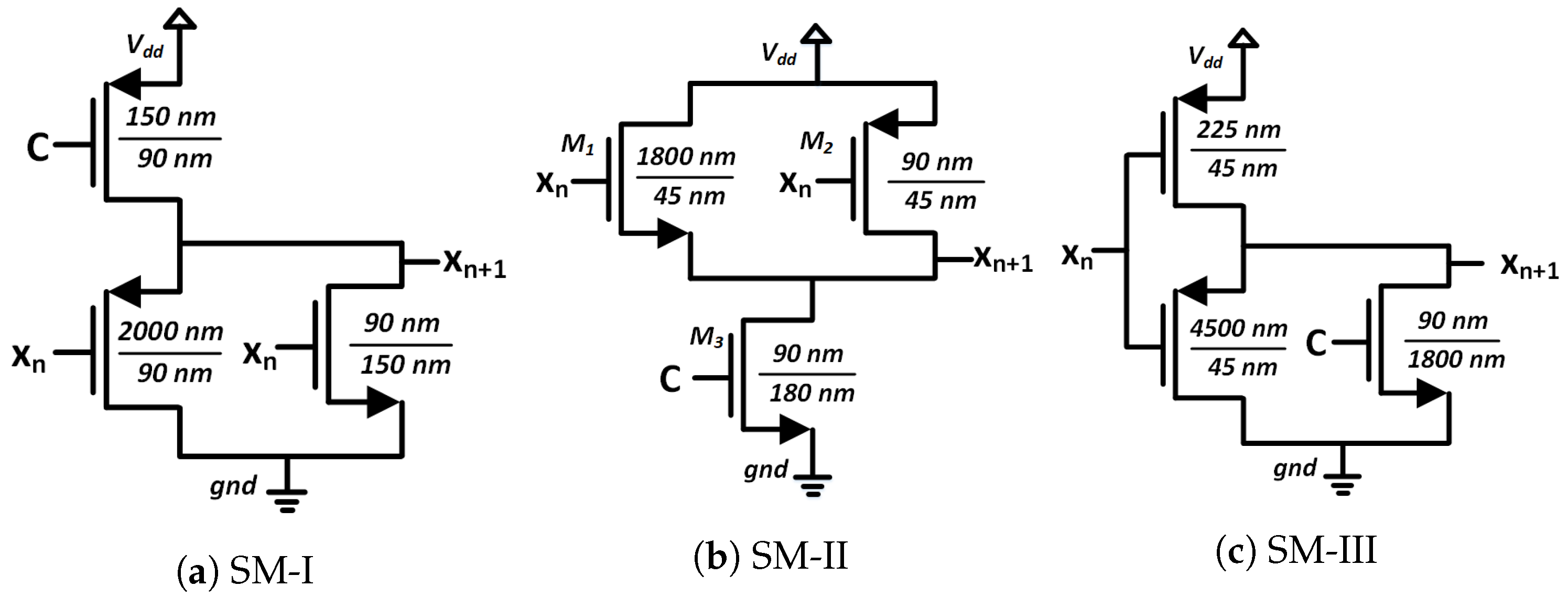
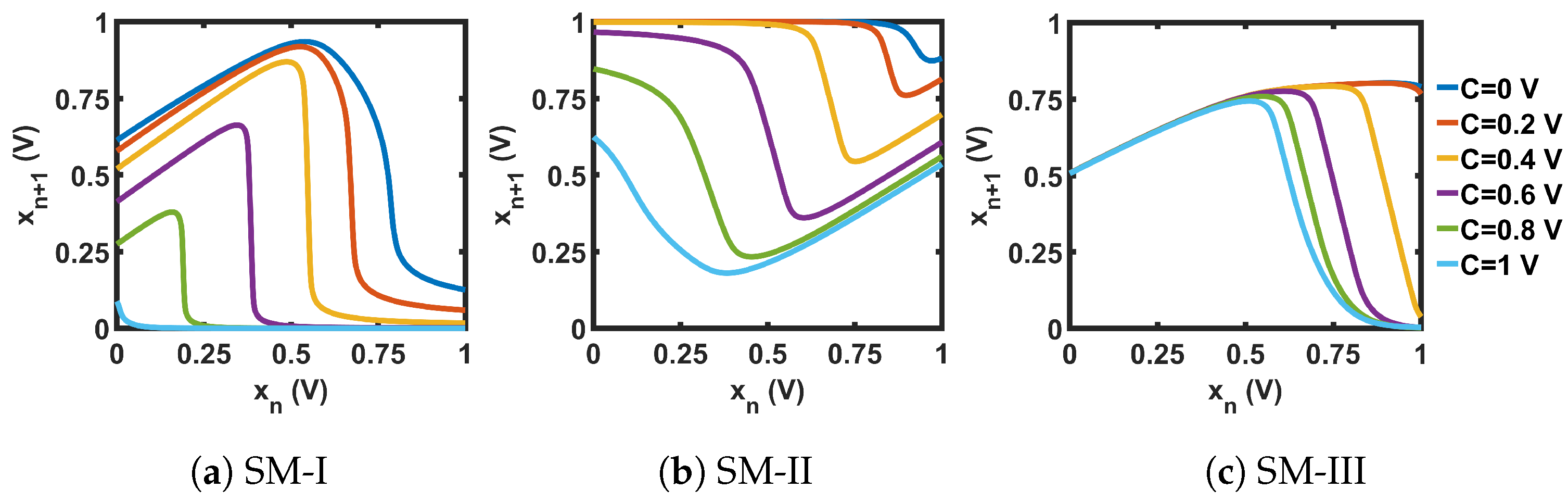
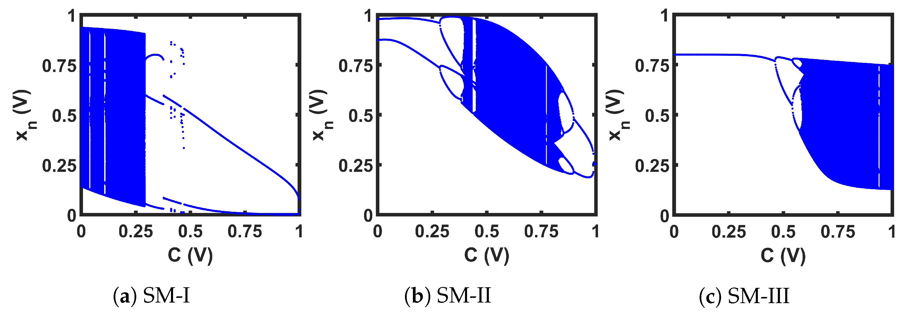
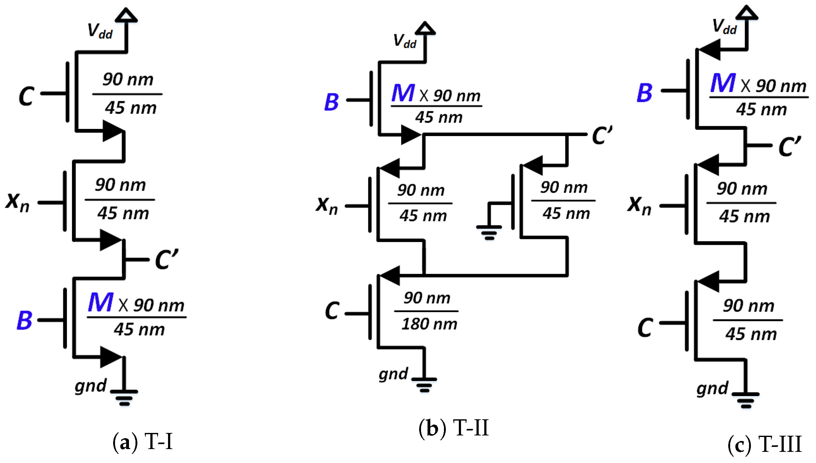
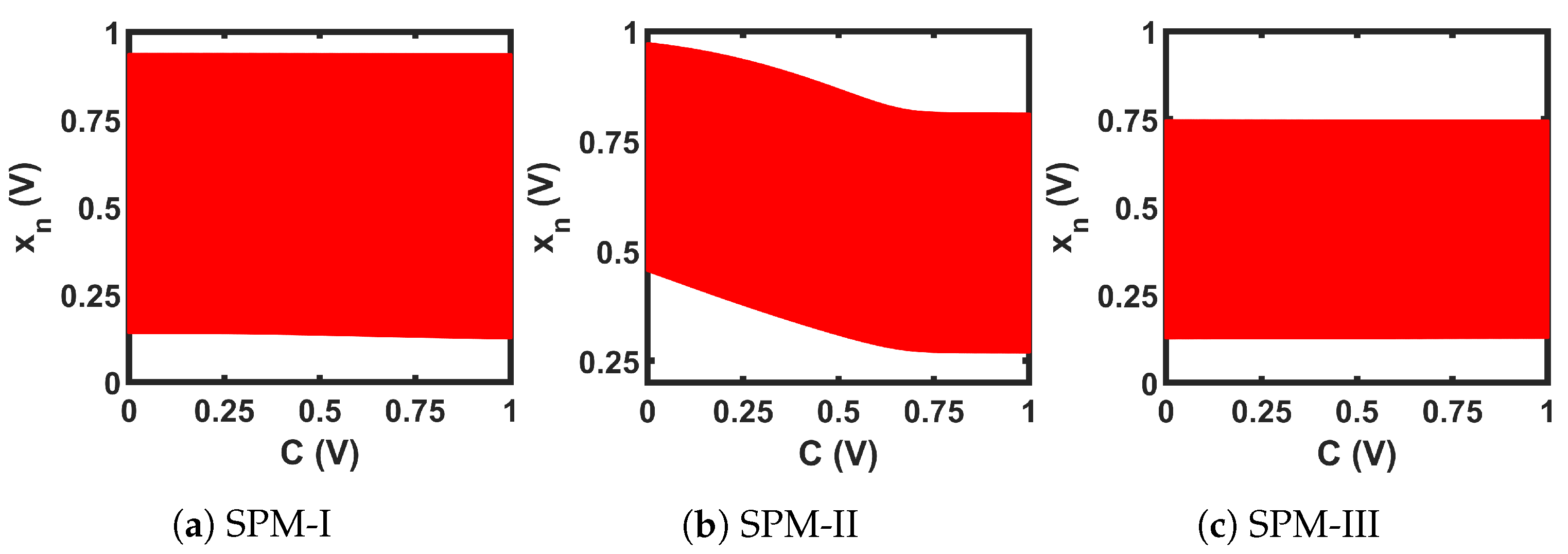
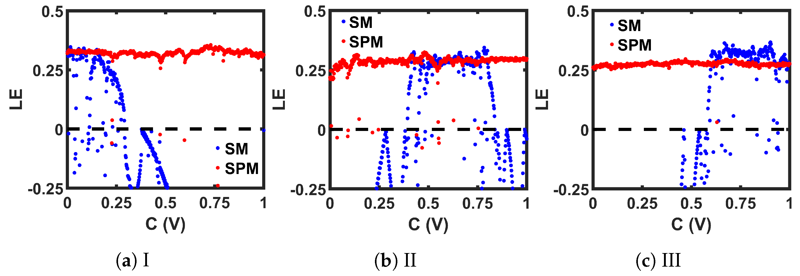
5. CMOS Implementation
6. Hardware Efficiency
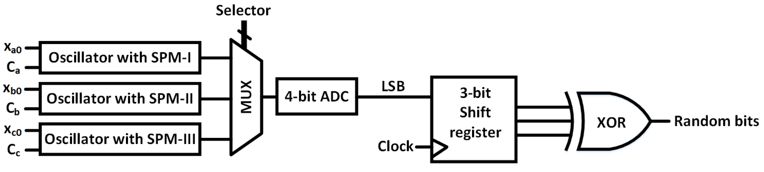
7. Application
7.1. Design of RNG
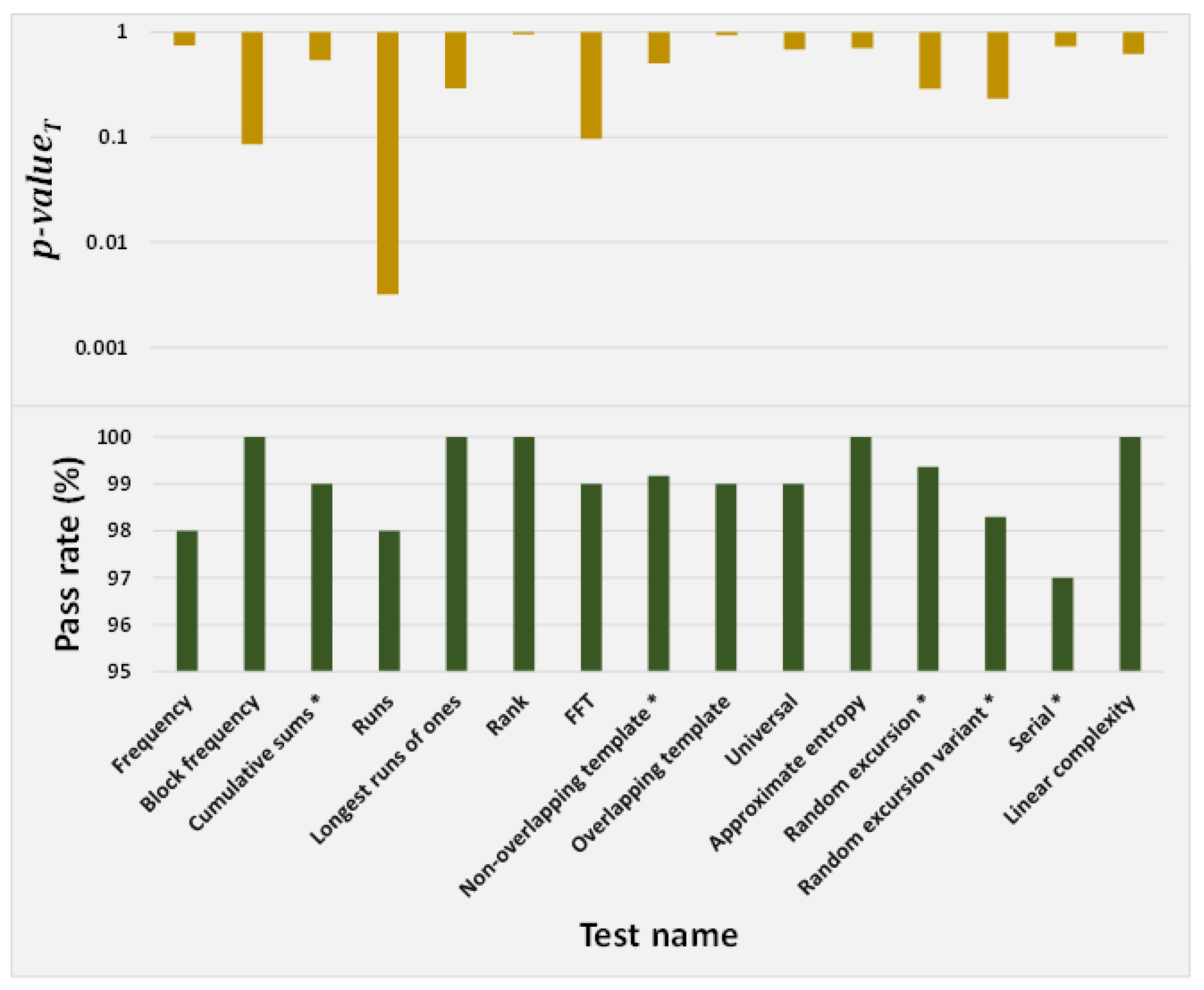
7.2. NIST
7.3. Hardware Considerations
8. Conclusions
Author Contributions
Funding
Data Availability Statement
Conflicts of Interest
References
- Hirsch, M.W.; Smale, S.; Devaney, R.L. Differential Equations, Dynamical Systems, and an Introduction to Chaos; Academic Press: Cambridge, MA, USA, 2012. [Google Scholar]
- Strogatz, S.H. Nonlinear Dynamics and Chaos: With Applications to Physics, Biology, Chemistry, and Engineering; CRC Press: Boca Raton, FL, USA, 2018. [Google Scholar]
- Csernák, G.; Stépán, G. Digital control as source of chaotic behavior. Int. J. Bifurc. Chaos 2010, 20, 1365–1378. [Google Scholar] [CrossRef]
- Poincaré, H. The Three-Body Problem and the Equations of Dynamics: Poincaré’s Foundational Work on Dynamical Systems Theory; Springer: Berlin/Heidelberg, Germany, 2017; Volume 443. [Google Scholar]
- Muthuswamy, B.; Banerjee, S. A Route to Chaos Using FPGAs; Springer: Berlin/Heidelberg, Germany, 2015. [Google Scholar]
- Lorenz, E.N. Deterministic nonperiodic flow. J. Atmos. Sci. 1963, 20, 130–141. [Google Scholar] [CrossRef]
- Hua, Z.; Zhou, Y. Dynamic parameter-control chaotic system. IEEE Trans. Cybern. 2015, 46, 3330–3341. [Google Scholar] [CrossRef]
- Zhou, Y.; Hua, Z.; Pun, C.M.; Chen, C.P. Cascade chaotic system with applications. IEEE Trans. Cybern. 2014, 45, 2001–2012. [Google Scholar] [CrossRef] [PubMed]
- Al-Shameri, W.F.H. Dynamical properties of the Hénon mapping. Int. J. Math. Anal. 2012, 6, 2419–2430. [Google Scholar]
- Gonzales, O.A.; Han, G.; De Gyvez, J.P.; Sánchez-Sinencio, E. Lorenz-based chaotic cryptosystem: A monolithic implementation. IEEE Trans. Circuits Syst. Fundam. Theory Appl. 2000, 47, 1243–1247. [Google Scholar] [CrossRef]
- Paul, P.S.; Hardy, P.; Sadia, M.; Hasan, M.S. A 2D Chaotic Oscillator for Analog IC. IEEE Open J. Circuits Syst. 2022, 3, 263–273. [Google Scholar] [CrossRef]
- Hua, Z.; Zhou, Y.; Pun, C.M.; Chen, C.P. 2D Sine Logistic modulation map for image encryption. Inf. Sci. 2015, 297, 80–94. [Google Scholar] [CrossRef]
- Zhu, H.; Zhao, Y.; Song, Y. 2D logistic-modulated-sine-coupling-logistic chaotic map for image encryption. IEEE Access 2019, 7, 14081–14098. [Google Scholar] [CrossRef]
- Gleick, J. Chaos: Making a New Science; Penguin: Westminster, UK, 2008. [Google Scholar]
- Zhou, Y.; Bao, L.; Chen, C.P. A new 1D chaotic system for image encryption. Signal Process. 2014, 97, 172–182. [Google Scholar] [CrossRef]
- El-Mowafy, M.; Gharghory, S.; Abo-Elsoud, M.; Obayya, M.; Allah, M.F. Chaos Based Encryption Technique for Compressed H264/AVC Videos. IEEE Access 2022, 10, 124002–124016. [Google Scholar] [CrossRef]
- Song, W.; Fu, C.; Zheng, Y.; Cao, L.; Tie, M.; Sham, C.W. Protection of image ROI using chaos-based encryption and DCNN-based object detection. Neural Comput. Appl. 2022, 34, 5743–5756. [Google Scholar] [CrossRef]
- Fridrich, J. Image encryption based on chaotic maps. In Proceedings of the 1997 IEEE International Conference on Systems, Man, and Cybernetics. Computational Cybernetics and Simulation, Orlando, FL, USA, 12–15 October 1997; IEEE: New York, NY, USA, 1997; Volume 2, pp. 1105–1110. [Google Scholar]
- Guo, J.I. A new chaotic key-based design for image encryption and decryption. In Proceedings of the 2000 IEEE International Symposium on Circuits and Systems (ISCAS), Geneva, Switzerland, 28–31 May 2000; IEEE: New York, NY, USA, 2000; Volume 4, pp. 49–52. [Google Scholar]
- Sobhy, M.I.; Shehata, A.E. Chaotic algorithms for data encryption. In Proceedings of the 2001 IEEE International Conference on Acoustics, Speech, and Signal Processing, Salt Lake City, UT, USA, 7–11 May 2001; Proceedings (Cat. No. 01CH37221). IEEE: New York, NY, USA, 2001; Volume 2, pp. 997–1000. [Google Scholar]
- Jakimoski, G.; Kocarev, L. Analysis of some recently proposed chaos-based encryption algorithms. Phys. Lett. 2001, 291, 381–384. [Google Scholar] [CrossRef]
- Paul, P.S.; Sadia, M.; Hasan, M.S. Design of a Dynamic Parameter-Controlled Chaotic-PRNG in a 65 nm CMOS process. In Proceedings of the 2020 IEEE 14th Dallas Circuits and Systems Conference (DCAS), Dallas, TX, USA, 15–16 November 2020; IEEE: New York, NY, USA, 2020; pp. 1–4. [Google Scholar]
- Agrawal, R.; Bu, L.; Del Rosario, E.; Kinsy, M.A. Towards Programmable All-Digital True Random Number Generator. In Proceedings of the 2020 on Great Lakes Symposium on VLSI, Virtual Event, 7–9 September 2020; pp. 53–58. [Google Scholar]
- Patidar, V.; Sud, K.K.; Pareek, N.K. A pseudo random bit generator based on chaotic logistic map and its statistical testing. Informatica 2009, 33, 441–452. [Google Scholar]
- Hamdi, M.; Rhouma, R.; Belghith, S. A very efficient pseudo-random number generator based on chaotic maps and s-box tables. Int. Comput. Electr. Autom. Control Inf. Eng. 2015, 9, 481–485. [Google Scholar]
- Tutueva, A.V.; Butusov, D.N.; Pesterev, D.O.; Belkin, D.A.; Ryzhov, N.G. Novel normalization technique for chaotic Pseudo-random number generators based on semi-implicit ODE solvers. In Proceedings of the 2017 International Conference Quality Management, Transport and Information Security, Information Technologies (IT&QM&IS), Saint Petersburg, Russia, 24–30 September 2017; IEEE: New York, NY, USA, 2017; pp. 292–295. [Google Scholar]
- Nardo, L.G.; Nepomuceno, E.G.; Arias-Garcia, J.; Butusov, D.N. Image encryption using finite-precision error. Chaos Solitons Fractals 2019, 123, 69–78. [Google Scholar] [CrossRef]
- Wang, L.; Cheng, H. Pseudo-random number generator based on logistic chaotic system. Entropy 2019, 21, 960. [Google Scholar] [CrossRef]
- Garcia-Bosque, M.; Pérez-Resa, A.; Sánchez-Azqueta, C.; Celma, S. A new randomness-enhancement method for chaos-based cryptosystem. In Proceedings of the 2018 IEEE 9th Latin American Symposium on Circuits & Systems (LASCAS), Puerto Vallarta, Mexico, 25–28 February 2018; IEEE: New York, NY, USA, 2018; pp. 1–4. [Google Scholar]
- Min, L.; Hu, K.; Zhang, L.; Zhang, Y. Study on pseudorandomness of some pseudorandom number generators with application. In Proceedings of the 2013 Ninth International Conference on Computational Intelligence and Security, Emeishan, China, 14–15 December 2013; IEEE: New York, NY, USA, 2013; pp. 569–574. [Google Scholar]
- Kia, B.; Jahed-Motiagh, M.R. A novel dynamically reconfigurable logic block based on chaos. Ifac Proc. Vol. 2006, 39, 372–377. [Google Scholar] [CrossRef]
- Pourshaghaghi, H.R.; Kia, B.; Ditto, W.; Jahed-Motlagh, M.R. Reconfigurable logic blocks based on a chaotic Chua circuit. Chaos Solitons Fractals 2009, 41, 233–244. [Google Scholar] [CrossRef]
- Gołofit, K.; Wieczorek, P.Z. Chaos-Based Physical Unclonable Functions. Appl. Sci. 2019, 9, 991. [Google Scholar] [CrossRef]
- Shen, J.; Huang, C.; Cheng, H. Design, Implementation and Analysis of PUF Structure Based on Chaos. In Proceedings of the 2021 International Conference on Communications, Information System and Computer Engineering (CISCE), Vitural, 14–16 May 2021; IEEE: New York, NY, USA, 2021; pp. 356–360. [Google Scholar]
- Kalanadhabhatta, S.; Kumar, D.; Anumandla, K.K.; Reddy, S.A.; Acharyya, A. PUF-based secure chaotic random number generator design methodology. IEEE Trans. Very Large Scale Integr. (Vlsi) Syst. 2020, 28, 1740–1744. [Google Scholar] [CrossRef]
- Illuri, B.; Jose, D. Design and implementation of hybrid integration of cognitive learning and chaotic countermeasures for side channel attacks. J. Ambient. Intell. Humaniz. Comput. 2021, 12, 5427–5441. [Google Scholar] [CrossRef]
- Bohl, J.; Yan, L.K.; Rose, G.S. A two-dimensional chaotic logic gate for improved computer security. In Proceedings of the 2015 IEEE 58th International Midwest Symposium on Circuits and Systems (MWSCAS), Fort Collins, CO, USA, 2–5 August 2015; IEEE: New York, NY, USA, 2015; pp. 1–4. [Google Scholar]
- Popp, T.; Mangard, S.; Oswald, E. Power analysis attacks and countermeasures. IEEE Des. Test Comput. 2007, 24, 535–543. [Google Scholar] [CrossRef]
- Hua, Z.; Zhou, Y. Exponential chaotic model for generating robust chaos. IEEE Trans. Syst. Man Cybern. Syst. 2019, 51, 3713–3724. [Google Scholar] [CrossRef]
- Ott, E.; Grebogi, C.; Yorke, J.A. Controlling chaotic dynamical systems. In Chaos: Soviet-American Perspective on Nonlinear Science; American Institute of Physics: College Park, MD, USA, 1990; pp. 153–172. [Google Scholar]
- Zaher, A.A.; Abu-Rezq, A. On the design of chaos-based secure communication systems. Commun. Nonlinear Sci. Numer. Simul. 2011, 16, 3721–3737. [Google Scholar] [CrossRef]
- Wang, S.; Kuang, J.; Li, J.; Luo, Y.; Lu, H.; Hu, G. Chaos-based secure communications in a large community. Phys. Rev. 2002, 66, 065202. [Google Scholar] [CrossRef] [PubMed]
- Rose, G.S. A chaos-based arithmetic logic unit and implications for obfuscation. In Proceedings of the 2014 IEEE Computer Society Annual Symposium on VLSI, Tampa, FL, USA, 9–11 July 2014; IEEE: New York, NY, USA, 2014; pp. 54–58. [Google Scholar]
- Sidhu, S.; Mohd, B.J.; Hayajneh, T. Hardware security in IoT devices with emphasis on hardware Trojans. J. Sens. Actuator Netw. 2019, 8, 42. [Google Scholar] [CrossRef]
- Zhao, H.; Njilla, L. Hardware assisted chaos based iot authentication. In Proceedings of the 2019 IEEE 16th International Conference on Networking, Sensing and Control (ICNSC), Banff, AL, Canada, 9–11May 2019; IEEE: New York, NY, USA, 2019; pp. 169–174. [Google Scholar]
- Ilyas, B.; Raouf, S.M.; Abdelkader, S.; Camel, T.; Said, S.; Lei, H. An Efficient and Reliable Chaos-Based IoT Security Core for UDP/IP Wireless Communication. IEEE Access 2022, 10, 49625–49656. [Google Scholar] [CrossRef]
- Shehadeh, Y.E.H.; Hogrefe, D. A survey on secret key generation mechanisms on the physical layer in wireless networks. Secur. Commun. Netw. 2015, 8, 332–341. [Google Scholar] [CrossRef]
- Kornaros, G. Hardware-assisted Machine Learning in Resource-constrained IoT Environments for Security: Review and Future Prospective. IEEE Access 2022, 10, 58603–58622. [Google Scholar] [CrossRef]
- Zheng, Y.; Liu, W.; Gu, C.; Chang, C.H. PUF-based mutual authentication and key exchange protocol for peer-to-peer IoT applications. IEEE Trans. Dependable Secur. Comput. 2022. [Google Scholar] [CrossRef]
- Cabrera-Gutiérrez, A.J.; Castillo, E.; Escobar-Molero, A.; Alvarez-Bermejo, J.A.; Morales, D.P.; Parrilla, L. Integration of Hardware Security Modules and Permissioned Blockchain in Industrial IoT Networks. IEEE Access 2022, 10, 114331–114345. [Google Scholar] [CrossRef]
- Phalak, K.; Ash-Saki, A.; Alam, M.; Topaloglu, R.O.; Ghosh, S. Quantum puf for security and trust in quantum computing. IEEE J. Emerg. Sel. Top. Circuits Syst. 2021, 11, 333–342. [Google Scholar] [CrossRef]
- Yu, F.; Li, L.; Tang, Q.; Cai, S.; Song, Y.; Xu, Q. A survey on true random number generators based on chaos. Discret. Dyn. Nat. Soc. 2019, 2019, 2545123. [Google Scholar] [CrossRef]
- Hasan, M.S.; Paul, P.S.; Dhungel, A.; Sadia, M.; Hossain, M.R. Design, Analysis, and Application of Flipped Product Chaotic System. IEEE Access 2022, 10, 125181–125193. [Google Scholar] [CrossRef]
- Méndez-Ramírez, R.D.; Arellano-Delgado, A.; Murillo-Escobar, M.A.; Cruz-Hernández, C. A New 4D Hyperchaotic System and Its Analog and Digital Implementation. Electronics 2021, 10, 1793. [Google Scholar] [CrossRef]
- Lopez-Hernandez, J.; Diaz-Mendez, A.; Vazquez-Medina, R.; Alejos-Palomares, R. Analog current-mode implementation of a logistic-map based chaos generator. In Proceedings of the 2009 52nd IEEE International Midwest Symposium on Circuits and Systems, Cancun, Mexico, 2–5 August 2009; IEEE: New York, NY, USA, 2009; pp. 812–814. [Google Scholar]
- Farfan-Pelaez, A.; Del-Moral-Hernández, E.; Navarro, J.; Van Noije, W. A CMOS Implementation of the Sine-circle Map. In Proceedings of the 48th Midwest Symposium on Circuits and Systems, Cincinnati, OH, USA, 7–10 August 2005; IEEE: New York, NY, USA, 2005; pp. 1502–1505. [Google Scholar]
- Callegari, S.; Setti, G.; Langlois, P.J. A CMOS tailed tent map for the generation of uniformly distributed chaotic sequences. In Proceedings of the 1997 IEEE International Symposium on Circuits and Systems (ISCAS), Hong Kong, China, 9–12 1997; IEEE: New York, NY, USA, 1997; Volume 2, pp. 781–784. [Google Scholar]
- Dudek, P.; Juncu, V. Compact discrete-time chaos generator circuit. Electron. Lett. 2003, 39, 1431–1432. [Google Scholar] [CrossRef]
- Dudek, P.; Juncu, V. An area and power efficient discrete-time chaos generator circuit. In Proceedings of the Proceedings of the 2005 European Conference on Circuit Theory and Design, Cork, UK, 29 August–1 September 2005; IEEE: New York, NY, USA, 2005; Volume 2, pp. 2–87. [Google Scholar]
- Paul, P.S.; Sadia, M.; Hossain, M.R.; Muldrey, B.; Hasan, M.S. Cascading CMOS-Based Chaotic Maps for Improved Performance and Its Application in Efficient RNG Design. IEEE Access 2022, 10, 33758–33770. [Google Scholar] [CrossRef]
- Sadia, M.; Paul, P.S.; Hossain, M.R.; Muldrey, B.; Hasan, M.S. Robust Chaos with Novel 4-Transistor Maps. IEEE Trans. Circuits Syst. Express Briefs 2022. [Google Scholar] [CrossRef]
- Hasan, M.S.; Paul, P.S.; Sadia, M.; Hossain, M.R. Integrated Circuit Design of an Improved Discrete Chaotic Map by Averaging Multiple Seed Maps. In Proceedings of the SoutheastCon 2021, Atlanta, GA, USA, 10–13 March 2021; IEEE: New York, NY, USA, 2021; pp. 1–6. [Google Scholar]
- Paul, P.S.; Dhungel, A.; Sadia, M.; Hossain, M.R.; Muldrey, B.; Hasan, M.S. Self-Parameterized Chaotic Map: A Hardware-efficient Scheme Providing Wide Chaotic Range. In Proceedings of the 2021 28th IEEE International Conference on Electronics, Circuits, and Systems (ICECS), Dubai, United Arab Emirates, 28 November–1 December 2021; IEEE: New York, NY, USA, 2021; pp. 1–5. [Google Scholar]
- Zeraoulia, E. Robust Chaos and Its Applications; World Scientific: Singapore, 2012; Volume 79. [Google Scholar]
- Wolf, A.; Swift, J.B.; Swinney, H.L.; Vastano, J.A. Determining Lyapunov exponents from a time series. Phys. Nonlinear Phenom. 1985, 16, 285–317. [Google Scholar] [CrossRef]
- Grassberger, P.; Procaccia, I. Characterization of strange attractors. Phys. Rev. Lett. 1983, 50, 346. [Google Scholar] [CrossRef]
- Pincus, S.M. Approximate entropy as a measure of system complexity. Proc. Natl. Acad. Sci. USA 1991, 88, 2297–2301. [Google Scholar] [CrossRef] [PubMed]
- MathWorks. Approximate Entropy. 2022. Available online: https://www.mathworks.com/help/predmaint/ref/approximateentropy.html (accessed on 2 January 2023).
- MathWorks. Characterize the Rate of Separation of Infinitesimally Close Trajectories. 2021. Available online: https://www.mathworks.com/help/predmaint/ref/lyapunovexponent.html (accessed on 10 December 2022).
- Hua, Z.; Zhou, B.; Zhou, Y. Sine chaotification model for enhancing chaos and its hardware implementation. IEEE Trans. Ind. Electron. 2018, 66, 1273–1284. [Google Scholar] [CrossRef]
- Rukhin, A.; Soto, J.; Nechvatal, J.; Smid, M.; Barker, E. A Statistical Test Suite for Random and Pseudorandom Number Generators for Cryptographic Applications; Technical Report; Booz-allen and Hamilton inc Mclean va: McLean, VA, USA, 2001. [Google Scholar]
- Cicek, I.; Pusane, A.E.; Dundar, G. A novel design method for discrete time chaos based true random number generators. Integration 2014, 47, 38–47. [Google Scholar] [CrossRef]
- Shanta, A.S.; Majumder, M.B.; Hasan, M.S.; Rose, G.S. Physically unclonable and reconfigurable computing system (purcs) for hardware security applications. IEEE Trans. Comput. Aided Des. Integr. Circuits Syst. 2020, 40, 405–418. [Google Scholar] [CrossRef]
- Juncu, V.; Rafiei-Naeini, M.; Dudek, P. Integrated circuit implementation of a compact discrete-time chaos generator. Analog. Integr. Circuits Signal Process. 2006, 46, 275–280. [Google Scholar] [CrossRef]
- Kia, B.; Mobley, K.; Ditto, W.L. An integrated circuit design for a dynamics-based reconfigurable logic block. IEEE Trans. Circuits Syst. Express Briefs 2017, 64, 715–719. [Google Scholar] [CrossRef]


| Map | Analytical Expression | Output Range | Control Parameter Range | Chaotic Range |
|---|---|---|---|---|
| Name | , | , | , | |
| Logistic | [0, 1] | [0, 1] | [0.9, 1] | |
| Sine | [0, 1] | [0, 1] | [0.87, 1] | |
| Tent | [0, 1] | [0, 1] | [0.52, 0.99] |
| Map | Selected Parameter Values | Analytical Expression |
|---|---|---|
| Name | M, B | |
| SPM-Logistic | M = 0.01, B = 0.975 | |
| SPM-Sine | M = 0.01, B = 0.96 | |
| SPM-Tent | M = 0.125, B = 0.74 |
Disclaimer/Publisher’s Note: The statements, opinions and data contained in all publications are solely those of the individual author(s) and contributor(s) and not of MDPI and/or the editor(s). MDPI and/or the editor(s) disclaim responsibility for any injury to people or property resulting from any ideas, methods, instructions or products referred to in the content. |
© 2023 by the authors. Licensee MDPI, Basel, Switzerland. This article is an open access article distributed under the terms and conditions of the Creative Commons Attribution (CC BY) license (https://creativecommons.org/licenses/by/4.0/).
Share and Cite
Paul, P.S.; Dhungel, A.; Sadia, M.; Hossain, M.R.; Hasan, M.S. Self-Parameterized Chaotic Map for Low-Cost Robust Chaos. J. Low Power Electron. Appl. 2023, 13, 18. https://doi.org/10.3390/jlpea13010018
Paul PS, Dhungel A, Sadia M, Hossain MR, Hasan MS. Self-Parameterized Chaotic Map for Low-Cost Robust Chaos. Journal of Low Power Electronics and Applications. 2023; 13(1):18. https://doi.org/10.3390/jlpea13010018
Chicago/Turabian StylePaul, Partha Sarathi, Anurag Dhungel, Maisha Sadia, Md Razuan Hossain, and Md Sakib Hasan. 2023. "Self-Parameterized Chaotic Map for Low-Cost Robust Chaos" Journal of Low Power Electronics and Applications 13, no. 1: 18. https://doi.org/10.3390/jlpea13010018
APA StylePaul, P. S., Dhungel, A., Sadia, M., Hossain, M. R., & Hasan, M. S. (2023). Self-Parameterized Chaotic Map for Low-Cost Robust Chaos. Journal of Low Power Electronics and Applications, 13(1), 18. https://doi.org/10.3390/jlpea13010018