Article

Towards Low-Power Machine Learning Architectures Inspired by Brain Neuromodulatory Signalling

1
Electrical & Computer Engineering, Brigham Young University, Provo, UT 84602, USA
2
Computer Science, Brigham Young University, Provo, UT 84602, USA
3
Cellular Biology and Physiology, Center for Neuroscience, Provo, UT 84602, USA
*
Author to whom correspondence should be addressed.
These authors contributed equally to this work.
J. Low Power Electron. Appl. 2022, 12(4), 59; https://doi.org/10.3390/jlpea12040059
Submission received: 30 September 2022 / Revised: 22 October 2022 / Accepted: 1 November 2022 / Published: 4 November 2022

Abstract

:
We present a transfer learning method inspired by modulatory neurotransmitter mechanisms in biological brains and explore applications for neuromorphic hardware. In this method, the pre-trained weights of an artificial neural network are held constant and a new, similar task is learned by manipulating the firing sensitivity of each neuron via a supplemental bias input. We refer to this as neuromodulatory tuning (NT). We demonstrate empirically that neuromodulatory tuning produces results comparable with traditional fine-tuning (TFT) methods in the domain of image recognition in both feed-forward deep learning and spiking neural network architectures. In our tests, NT reduced the number of parameters to be trained by four orders of magnitude as compared with traditional fine-tuning methods. We further demonstrate that neuromodulatory tuning can be implemented in analog hardware as a current source with a variable supply voltage. Our analog neuron design implements the leaky integrate-and-fire model with three bi-directional binary-scaled current sources comprising the synapse. Signals approximating modulatory neurotransmitter mechanisms are applied via adjustable power domains associated with each synapse. We validate the feasibility of the circuit design using high-fidelity simulation tools and propose an efficient implementation of neuromodulatory tuning using integrated analog circuits that consume significantly less power than digital hardware (GPU/CPU).

1. Introduction

Analog CMOS hardware has the potential to reduce energy consumption of deep neural networks by orders of magnitude, but the in situ training of networks implemented on such hardware is challenging. Once the chip has been programmed with the correct weight values for a task, typically no further learning occurs. We introduce a biologically-inspired knowledge transfer approach for neural networks that offers potential for in situ learning on the physical chip. In our method, the weight matrices of a spiking neural network [1,2,3,4,5] are initialized with values learned via offline (i.e., off-chip) methods, and the system is exposed to an analogous—but distinct—learning task. The bias inputs of the chip’s spiking neurons are manipulated such that the network’s outputs adapt to the new learning task.
This approach has applications for autonomous, power-constrained devices that must adapt to unanticipated circumstances, including vision and navigation in unmanned aerial vehicles (UAVs) deployed into unpredictable environments; fine-grained haptic controls for robotic manipulators; dynamically adaptive prosthetic devices; and bio-cybernetic interfaces. In these real-world domains, the system must deploy with initial knowledge relevant to its target environment, then adapt to near-optimal behavior given minimal training examples, a feat beyond the capability of current learning algorithms or hardware platforms. Neuromodulatory tuning offers a path toward implementing such abilities on physical CMOS chips. The key contributions of our work are as follows:
  • We introduce a novel transfer learning variant, called neuromodulatory tuning, that is able to match the performance of traditional fine-tuning approaches with orders of magnitude fewer weight updates. This lends itself naturally to easier, lower power implementation on physical chips, especially because the proposed CMOS implementation of our the fine-tuning method does not involve writing to memory hardware.
  • We provide a biologically-inspired motivation for this tuning method based on recent findings in neuroscience, and discuss additional insights gleaned from modulatory neurotransmitter behaviors in biological brains that may prove valuable for neuromorphic computing hardware.
  • We demonstrate in both traditional (non-analog) feed-forward architectures and spiking neural network simulations that neuromodulatory tuning methods are able to approach or exceed the performance of traditional fine-tuning methods on a number of transfer learning tasks in the domain of image recognition, while overall task performance must still be improved, the trends and potential of the method are encouraging.
  • We outline the mechanisms by which neuromodulatory tuning can feasibly be implemented on CMOS hardware. We present an analog spiking neuron with neuromodulatory tuning capabilities. Post-layout simulations demonstrate energy/spike rates as low as 1.08 pJ.
The remainder of this paper adheres to the following structure: We begin by providing a general background on transfer learning, artificial neural networks, and neuromorphic hardware in Section 2. We then outline the motivating principles and neurobiological foundations of the current work (Section 3.1) and present our biologically inspired tuning method (Section 3.2). A preliminary analysis follows (Section 4), showing performance comparisons of NT versus TFT in digital computation environments across a variety of learning rates and transfer tasks. Lastly, we present our spiking neuron design (Section 5) with confirming evidence that our neuromodulatory tuning method can be used as an acceptable proxy for traditional fine-tuning in analog CMOS environments (Section 6). Conclusions are presented in Section 7.

2. Background

The current study lies at the intersection of three prodigious research fields: Transfer learning (Section 2.1), spiking neural networks (Section 2.2), and neuromorphic computing (Section 2.3). We outline key principles of each below. Our method also draws heavily on recent discoveries in neuroscience, documented alongside the motivating principles of this research in Section 3.1.

2.1. Transfer Learning

Transfer learning allows a network trained for one task to learn a new, similar task with less computational complexity than fully retraining the network. The field includes a broad range of techniques ranging from weighting, importance sampling, and domain adaptation in unsupervised contexts [6,7,8,9,10,11], to fine-tuning and multi-task learning in supervised settings [12,13,14,15,16,17,18]. Recent work in few-shot, one-shot, and zero-shot learning also contributes to this line of research [19,20,21,22].
Our approach can be combined with many of these methods, but is most closely related to feature learning from unsupervised data [13], whereby trained parameters from a related task are used to jump-start the learning process. Our method is distinct in that the activation sensitivity of individual neurons, rather than the strengths of their synaptic connections, are modified. In some sense, this can be viewed as a degenerate form of neural programming interface [23], in that activation patterns are modulated during each forward pass of the network; however, our method adjusts firing sensitivities via supplemental bias inputs rather than by overwriting output signals directly. Our work also has tangential relations to activation function learning [24], although we adjust firing sensitivity only, rather than changing the shape of the activation curve.
Parallel to our work, ref. [25] presented BitFit, which shows bias tuning is an effective sparse fine-tuning method that is competitive with traditional fine-tuning on Transformer-based Masked Language Models. Our work augments and expands upon the insights from this work in two key ways: We apply a bias tuning methodology much like [25] to a convolutional neural network in the domain of computer vision, where we discover that it is not able to match the performance of a traditional fine-tuning method, and we present a novel approach to bias tuning (neuromodulatory tuning) based on multiplicative rather than summative layer modifications, and demonstrate that this method is able to match traditional fine-tuning approaches.

2.2. Spiking Neural Networks

Spiking neural networks (SNNs) [1,3,4,26,27,28] are artificial neural networks that attempt to mimic temporal and synaptic behaviors of biological brains. Rather than using continuous activation functions, spiking neurons utilize a series of binary pulses, called a spike train [29], to propagate information forward in a brain-like manner. SNNs are particularly well-suited to implementation on analog/mixed-signal hardware, which naturally supports the high parallel sparse activation pathways common in such networks [30].
Despite these potential advantages and their strong parallels with biological brain behavior, SNNs have not gained as much recent prominence as traditional (digital) feed-forward networks, in part because of the difficulty of propagating gradient information backwards through a spike train [31]. One means to compensate for this is by training a traditional (non-spiking) network using back-propagation and then applying a transfer function to convert the learned weights into their SNN equivalents [32]. We leverage this idea in our work, but instead of applying a transfer function, we copy the non-spiking weights directly, then use neuromodulatory tuning to adapt them to a new learning task.
Recent works detailing the conversion of traditional feed-forward networks to SNNs use algorithms which modify weights, biases and activation thresholds of the network to create a SNN from a feed-forward network [33,34]. The difference between our work and others is that we do not train the network to match the behavior with existing feed-forward network. Instead, we seek to train network for different tasks. Therefore, we do not perform layer-wise comparison which is resource consuming. Moreover, our work tunes a single parameter per neuron which is far more implementable on physical chips compared to other more computationally expensive methods.

2.3. Neuromorphic Hardware

Neuromorphic hardware uses dedicated processing units to implement neuronal connections and firing behavior directly on a physical chip, rather than simulating them mathematically. Analog neuromorphic hardware has been shown to be more power efficient than traditional digital computation hardware, and does not suffer from the same bottleneck as Von Neuman computing [35,36,37,38,39,40,41,42]. Some designs take advantage of sub-threshold operation for ultra-low power neurons [43,44]. Further power reductions have been achieved through sparse temporal coding [30].
The temporal nature of spiking neural networks naturally lends itself to on-chip, biologically plausible learning methods. Spike-time-dependent plasticity (STDP) uses analog hardware to directly implement learning rules on chip. Several works have shown impressive learning accuracies using this method [29,35,45,46,47]. However, direct hardware implementations for learning rules consume large amounts of space and power, limiting its potential learning capacity. Our work bridges this gap by offering the possibility of on-chip learning with similar performance but reduced space and component requirements.

3. Neuromodulatory Tuning

Neuromodulatory tuning is a novel fine-tuning method based on recent discoveries in neuroscience. Neuronal transmission in biological brains is highly complex in timing and can occur either via rapidly terminating signals that influence only immediately connected cells (synaptic transmission), or via chemical signals that spread further away to simultaneously influence larger groups of neurons (volumetric transmission) [48,49]. Our work is motivated by and takes inspiration from this non-synaptic transmission method. Specifically, we observe that, rather than adjusting connection strengths between neurons directly, modulatory neurotransmitters impact system behavior by affecting the activation threshold of each neuron. Thus, a single trainable parameter, implemented in our case as a supplementary input, can be used in lieu of the large suite of trainable parameters typically employed during a fine-tuning process.

3.1. Biological Foundations

Modulatory neurotransmitters in biological brains use metabotropic g-protein coupled receptors as opposed to strictly ion conducting receptors propagate signals, and can include neurotransmitters such as the cathecholamines dopamine and norepinephrine [50,51,52,53,54]. Interestingly, glutamate is also used by neurons as a modulatory metabotropic signal, though it is largely discussed in the context of ion channel activity [55].
Artificial neural networks principally use neuronal ion channel activity, as represented by classical synapses, to represent synaptic strength. In contrast, metabotropic neuromodulators activate g-protein coupled receptors in neurons, whose downstream effectors can be stimulatory or inhibitory (depending on predefined cellular components) and work through a series of effectors that can amplify signals from traditional synaptic inputs, resulting in multiplicative tuning of the neuron’s inputs. This is considered a tuning process since these neurotransmitters often do not directly change the membrane potential, but instead change the activation threshold by modulating the channels receiving inputs. Our neuromodulatory tuning method simulates this increase or decrease in sensitivity by including additional inputs to the incoming signal, as shown in Section 5. In other words, neuromodulatory tuning increases a model’s sensitivity to specific pre-learned features, rather than changing the functions represented by those features. To our knowledge, this is the first application of volumetric, as opposed to strictly synaptic, mesolimbic attention modalities within an analog CMOS system.

3.2. Implementation

We simulate increased or decreased resting cell voltage via the introduction of a supplementary bias neuron for each network layer to be fine-tuned, as shown in Figure 1. The weights connecting this bias to neurons within each layer are initialized according to a random uniform distribution, and, if the number of output categories has changed from the original task, a new output layer is appended to the model. These additional bias weights are multiplied to the pre-trained weights in each layer of a network selected for fine tuning. The additional bias weights are then adjusted using standard back-propagation methods while all original weights from the pre-trained model are held fixed. This multiplicative bias method outperformed traditional additive bias, presented by [25], in experiments shown Table 1.
Alternately, neuromodulatory tuning can also be implemented by unfreezing only the existing bias weights of the pre-trained model, leaving all other weights fixed. We denote the additional bias neuron implementation as N T 1 , and denote this unfreezing bias weights implementation as N T 2 . Although the representational capacity of both methods is equivalent from a theoretical standpoint, we find that, empirically, introducing additional bias neurons ( N T 1 ) functions slightly better in deep feed-forward networks as shown in Table 2. Consequently, we use N T 1 in our experiments with feed-forward networks in Section 4. In spiking networks, we compare both implementations ( N T 1 and N T 2 ) and we find N T 1 performs better on STL-10 dataset, but has similar performance with N T 2 on Food-11 and BCCD as shown in our experiments with spiking networks in Section 6.1.

4. Modeling and Analysis

We first probe the capabilities and weaknesses of neuromodulatory tuning (NT) in a traditional deep learning setting. Using a pre-trained VGG-19 network architecture, we fine-tune the model on three image recognition tasks. VGG-19 was trained on ImageNet [56], an image classification dataset composed of 1000 different image categories. The first dataset we use in our evaluation is STL-10, a subset of ImageNet with only 10 image categories [57]. We expect traditional fine-tuning (TFT) and neuromodulatory tuning (NT) to achieve high accuracies on STL-10 since the data is a subset of the original training data. Next, we evaluate neuromodulatory tuning on a more difficult food classification task, Food-11 [58], which contains images of 11 different types of food none of which match any of ImageNet’s classes. Finally, we examine the capability of neuromodulatory tuning to learn blood cell classification (BCCD) [59], which is a task very distinct from ImageNet containing 4 classes of blood cells images. We hypothesize that as the difficulty of the tasks increase, NT will be less effective in tuning the model to solve the given task, but still comparable to TFT.
For simplicity, fine tuning is applied only to the VGG-19 classifier layers, a process which lowers the fine-tuned classification accuracy but facilitates our comparisons to spiking neural network implementations in Section 5.1. Additionally, it is common practice to only fine tune select layers of VGG models in recent literature [60,61]. We then apply neuromodulatory tuning to the same layers that were fine-tuned (i.e., classification layers only) and compare the performance of traditional fine tuning (TFT) to neuromodulatory tuning (NT), as shown in Table 3.
To visualize the comparison between neuromodulatory tuning (NT) and traditional fine-tuning (TFT), we create two model architectures, one with hyper-parameters configured for NT and the other for TFT. We use the existing train and validation partitions in the STL-10, Food-11 and BCCD datasets to train and evaluate the classifier layers of the pre-trained VGG-19 model. We resize the data in each of the datasets to be images of size 256 × 256 to be compatible with VGG-19. Using an NVIDIA GeForce RTX 2080 Ti GPU, we fine-tune both models for 10 epochs, with various training set sizes and learning rates.
We set the batch size to 64 training instances in all experiments with neural networks. The effect of batch size on model performance has been studied in depth in recent literature. Kandel and Castelli [62] study the effect of varying batch size and learning rate on VGG-16, and also provide a literature review which details several papers concerning the properties of training batch sizes. From these sources, it is clear that batch size and learning rates are dependent, but the measure of dependence often differs depending on the given task, model, and optimizer. Thus, we run a quick experimental analysis of the effect of batch size for a given learning rate on VGG-19 and the Food-11 dataset in Table 4. The learning rate for NT is set to be 0.01 and it is set to 0.0001 for TFT, since these learning rates performed well in preliminary results. As evident from the results in Table 4, we see that batch size does not effect the validation accuracy of NT or TFT models significantly. Therefore, we can fix batch size to 64 in the remainder of our experiments with varying learning rates.
To perform gradient descent we use Cross Entropy Loss and the Adam optimizer. After tuning, we iterate through the entire predefined validation set to find the mean loss and accuracy for a specific model (NT or TFT) and learning rate.
Our results show that algorithm performance between traditional fine-tuning (TFT) and neuromodulatory tuning (NT) is largely on par, a result that remains consistent across a wide variety of learning rates. Table 3 provide our experimental data that highlights the best-performing learning rates for NT (lr = 0.01) and TFT (lr = 0.0001). Interestingly, the optimal learning rate for each tuning algorithm differs, and the average performance of NT across multiple learning rates is higher than that of TFT. TFT achieves the highest validation accuracies overall, but critically, not by much. This is important because it means we can retain much of TFT’s learning accuracy while using four orders of magnitude fewer trainable parameters, a circumstance that makes NT far more feasible than TFT to implement on neuromorphic hardware.
Recognizing our success in the results presented above, we further reduced the number of tunable parameters. The reduction in parameters was biologically motivated such that each tunable parameter matches to a single neuron in the classifier layers of VGG-19. Specifically, our initial results as reported in Table 3 include a set of tunable parameters applied after the VGG-19 convolutional layers but before the data was passed into the VGG-19 classifier. Table 5 shows the same experiment repeated with this additional layer of parameters removed, resulting in an even smaller number of trainable parameters—a critical factor for potential implementation of such methods within the space constraints of physical analog chips. We found that this reduction in parameters did decrease the accuracy of the network on each task, but only slightly. As this reduced parameter count is more analogous to biological neuromodulatory transmitters, we use this NT configuration in future experiments in Section 5.1.

5. Methods

5.1. Neuromodulatory Tuning on Spike Neural Networks

The VGG-19 architecture is complex and difficult to implement in its entirety on a SNN architecture, in particular due to the large number of convolution and max pooling layers. Since our research goal is to explore the learning effect of neuromodulatory signalling on brain-like architecture, and not to replicate VGG-19, we apply the following simplification in our experiments: The feature layers of VGG-19 are retained in their original (digital) deep format. As illustrated in Figure 2, image inputs are passed through these layers to attain a feature embedding, which would normally be passed through to the VGG-19 classification layers. We replace the VGG-19 classification layers with a spiking neural network having the same number of layers and layer width. The weight matrices of these SNN-VGG classification layers are initialized to the same values as the pre-trained VGG-19 weights.
We implement our spiking neural network using core algorithm components outlined by leaky integrate-and-fire model [63], with the following adjustments:
  • Network update frequency minimization
  • Customized simple loss calculation method on network output

5.1.1. Update Frequency Minimization

A typical leaky integrate-and-fire neuron receives input over a set time span. During this time span, neurons must be updated multiple times to simulate temporal connectivity on the actual circuit [29,35,45,46,47], which greatly increases the computation costs of simulation. Since temporal connections are not a major factor in the VGG-19 image classification tasks, our update frequency for each neuron can be as small as 1 timestep for each task. Therefore, in our simulation for this experiment, we update neurons in each SNN layer exactly once.
Since we update neurons in each SNN layer exactly once, neurons will only fire at most once. As a consequence, argmax is not applicable on our output layer. Argmax chooses the maximum value from the output neurons as the true output, which make sure the output to be exactly one classification. In absent of argmax, network will start to output multiple classifications through activation of multiple neurons, which will be counted as mis-classification. Therefore, the network should not only activate the correct neuron, but it also should avoid the activation of incorrect neurons. Let n be the numbers of neurons which equals to numbers of classes in the tasks. Let p be the actual accuracy of random outputs, then:
p = 1 2 · 1 2 n 1 = 1 2 n
of which 1 2 is the possibility of the correct neuron activates and 1 2 n 1 is the possibilities of all incorrect neurons do not fire.

5.1.2. Simple Loss Calculation

For each neuron in our SNN output, one spike indicates an output of 1.0 and no spikes represents an output of 0.0. Therefore, the output of the SNN for each input will be an array consisting exclusive of values in {0.0, 1.0}. Due to the simplicity of the output as a binary array, we employ a customized simple gradient calculation method on the network output, calculated as follows:
loss = target output
This simple method fits our SNN simulation for this experiment, because of the binary output nature of our SNN. A binary output simply indicates whether a neuron fired or not. Losses on the binary output imply whether the neurons on the output layer have fired or not. Therefore, the polarity of the SNN output loss (i.e., whether it is positive or negative) is sufficient for basic training. We believe that other, more complex loss calculation methods have potential to perform better on these tasks, and that will be left to future explorations.

5.1.3. Gradient Calculation

Our network behaves according to the following equations:
v i = j = 0 n O j w i j + b i a i
O i = H ( v i ) I
H ( v ) = 1 , if   v θ 0 , otherwise
where v i is the voltage of the neuron i, w i j is the weight of the input given by neuron j to neuron i, b i is the additive bias of the neuron i, a i is the amplifier bias, O i is the output of neuron i calculated by our Heaviside function H times I, which represents a neuron’s output if fires, and θ is the activation threshold of neuron.
The gradient will then be calculated as:
g w i j = d O u t p u t d O i       d O i d H i       d H i d v i       d v i d w j · l o s s
g a i = d O u t p u t d O i       d O i d H i       d H i d v i       d v i d a i · l o s s
Since many researchers implement sigmoidal neurons, with steep sigmoid function, as a replacement for Heaviside step function, we can safely assume:
d H i d v i d S i g m o i d ( d v i ) d v i
The sigmoid method in popular machine learning libraries behaves as follows:
d S i g m o i d ( v ) d v = 1 + s , if   v θ , s 0 d , if   v θ , with   0 < d < 1 s , otherwise
where s approaches 0, but never reaches 0. Most of modern day techniques requires sigmoid to be steep, to minimize the window of v θ . Therefore, our method seeks to remove the influence of v θ by using customized sigmoid derivative σ :
d S i g m o i d ( v ) d v σ v = 1 , if   v θ s , otherwise , with   s 0
However, this σ function causes firing neurons to be adjusted 1 / s times faster than non-firing neurons. Such behavior becomes most problematic on physical chips, due to the fact that weight has its upper limit on physical chips. To make sure the weight adjustment speed on non-firing neurons matches firing neurons we amplified the gradient on non-firing neurons by 1 / s . Then, σ = 1 for all firing and non-firing neurons.
As a result, our gradient function becomes:
g w i j d O u t p u t d O i       d O i d H i       d v i d w i j · l o s s
g a i j d O u t p u t d O i       d O i d H i       d v i d a i · l o s s
Since d v i d w i j = O ( v j ) = H ( v j ) · I , and Heaviside step function produces 0 when v i < θ , the gradient chain will break when the Heaviside function outputs 0.
Therefore, our Heaviside step function on the simulation side is modified as:
H s i m ( v ) = 1 , if   v θ s , otherwise , with   s 0
If s is small enough as it approaches 0, s poses no influence on the accuracy of simulation comparing to hardware performance.

5.2. Neuromodulatory Tuning on Analog Hardware

One particularly advantageous aspect of neuromodulatory tuning (NT) is its suitability for implementation on analog neuromorphic hardware. The behavior of fine-tuned bias connections, implemented in digital simulations as additional bias neurons, can also be implemented in analog hardware as a current source with a variable supply voltage. This approach has the following advantages:
  • Minimal additional chip area required
  • Lower power consumption than digital hardware
  • No need to re-load weights to the on-chip memory
To probe this possibility, we use Cadence Virtuoso to explore the feasibility of a NT approach on simulated analog hardware. Our hardware is designed and simulated at the transistor level in TSMC 28-nm CMOS. The analog neuron implements the leaky integrate-and-fire model [63]. Six binary-scaled current sources make up the synapse. A current is driven onto a 50-fF capacitor to produce an integrated membrane voltage that is quantized by a dynamically clocked latched comparator. An adjustable delay line generates a 100-ns spike when the membrane voltage reaches the activation threshold and resets the membrane voltage by connecting the capacitor to ground via a pull-down transistor. A schematic diagram of our proposed neuron is shown in Figure 3.

5.2.1. Synapse Design

Each synapse operates at a supply voltage between 0.5 and 1 V. A higher supply increases the current in the synapse. The neuron core operates at a constant supply of 1 V. Adjusting the supply voltage of individual synapses or groups of synapses effectively changes the weights of the synapse connections. This change in behavior is analogous to the bias neurons in the software implementation and to what is observed biologically [53,54]. To make the synapse current dependent on the supply voltage V D D , we use a current mirror with a resistive load. The current through an N-type MOSFET is given by
I D S = 1 2 β ( V G S V t h ) 2
In a current mirror, the gate voltage V G is related to V D D by
V G = V D D I R S
Substituting (14) into (15) and solving for I results in
I = ( 4 β R S ( V D D V t h ) 1 ) + 2 β R S ( V D D V t h ) + 1 2 β R S 2
Equation (16) shows that the synapse current is a function of the supply voltage V D D , which we tune to adjust the weights. Figure 4 shows the neuron behavior when we vary V D D from 550 mV to 750 mV. The higher supply results in a larger current, producing more spikes.
The effect of a bias neuron with a weight of W b on a synapse with weights W s can be approximated as I ( W b + W s ) . The behavior of the analog implementation can be written as k I W where k represents the change in the synapse current due to adjusting V D D . If I W b = k W then the behavior of the two implementations is identical.

5.2.2. Neuron Core Design

A schematic of the neuron core is shown in Figure 5. The threshold comparator is implemented with the StrongARM topology. We choose a clocked topology to reduce static power, especially when compared to inverter based threshold detectors. Instead of a fixed-period clock, we only clock the comparator after an input spike or after an output spike. We use a 4-input NOR gate to generate the comparator clock. This ensures that power consumption is minimized in a network trained for minimal spiking activity. The membrane capacitance is always reset to V r e s t = 250 mV and the comparator has a fixed threshold of V t h , c o m p = 350 mV. We choose V r e s t to give V m e m at least 100 mV of swing without driving the synapse current sources into the triode region, even when the synapse power supply is 0.5 V. Once the membrane potential crosses the preset threshold, the spike generation circuit is triggered. The spike is generated using a self-reset DQ fip-flop with current-starved inverter-based delay cells between Q and reset. The delay cells utilize parasitic capacitance to increase delay so as to decrease the number of stages needed for a certain spike width.
The membrane capacitor is a custom 50-fF finger capacitor which occupies only 27 μ m 2 . Because the membrane capacitance is only 50 fF, the neuron needs an extremely large resistor for a sufficiently low leakage current. Instead of using a polysilicon resistor which would occupy large area, we implement a CMOS pseudo resistor using a PMOS transistor which occupies only 0.7 μ m × 0.5 μ m and achieves approximately 400 M Ω (Figure 6). The pseudo-resistor is implemented as two PMOS transistors connected in a transdiode configuration. The simplest of pseudo-resistors have an asymmetric resistance-voltage characteristic, making them unusable for this neuron because the membrane potential can go both above and below V r e s t , and must have the same up and down leakage current. To solve this, we use two psuedo-resistors in parallel with opposite connections polarities. This halves the effective resistance, but creates a symmetric resistance-voltage characteristic.

6. Results

Our long-term objective is to enable low-power analog learning behaviors in situ on physical analog chips. This requires both a viable mechanism for potential in situ learning that does not require large amounts of surface area for gradient calculations and a validated circuit design that can realistically implement that mechanism. We present neuromodulatory tuning as a possible mechanism for this objective, and here provide results showing its performance in simulated (digital) spiking neural networks (Section 6.1) and a full chip design for its eventual implementation on physical CMOS hardware (Section 6.2).

6.1. Neuromodulatory Tuning on Spiking Neural Networks

To validate the performance of neuromodulatory tuning in spiking neural networks (distinct from the traditional feed-foward networks shown in Section 4), we apply neuromodulatory tuning (NT) and traditional fine-tuning (TFT) to the SNN-VGG classification layers using the STL-10, Food-11, and BCCD datasets for comparison. We fix the batch size at 64 for all training, since our experiment with batch sizes (shown in Table 6) reveals that batch size does not impact the model performance dramatically. Both the Food-11 and BCCD datasets are singularly distinct from the ImageNet data [56] which was used to train VGG-19. VGG-19 therefore lacks output classes corresponding to labels from the Food-11 and BCCD datasets. To create the necessary output layer size, we added one extra fully connected layer at the end of each model. This extra layer functions as the output layer for corresponding classes in Food-11 and BCCD. Different from Food-11 and BCCD, STL-10 is a subset of ImageNet. Since VGG-19 is trained on ImageNet, VGG-19 contains classes that are contained within in STL-10 labels. Therefore, we do not add extra layers for the SNN STL-10 experiments. All SNN models were trained on an AMD Ryzen Threadripper 1920X 12-Core Processor. Results are shown in Table 7 and Table 8.
As expected, performance is poor when no tuning is applied. This is partially because SNN architectures, comprised of leaky integrate-and-fire neurons, differ drastically from traditional deep networks in both signal accumulation and signal propagation, resulting in almost 0% accuracy on all three transfer tasks. Tuning improves this accuracy, achieving up to 88% accuracy with TFT and 50% with NT on some tasks with certain learning rates. According to our results shown in Table 7, NT underperforms on the STL-10 dataset comparing to TFT, has equal performance to TFT on BCCD, and outperforms TFT on Food-11, which suggests that neuromodulatory tuning can positively impact learning behaviors on brain-like architectures.
Our performance comparison of the algorithms is influenced by differences between the three datasets. STL-10 is the subset of the dataset used to train VGG-19, so tasks in STL-10 is more native to the network. In contrast, Food11 and BCCD are foreign to the VGG-19 network, so those tasks will require VGG-19 to make adjustments in larger magnitudes or completely re-learn the task. Given that neuromodulatory tuning outperforms TFT on Food11, a foreign dataset, and that TFT requires changes of larger magnitudes, NT is superior for these cases. There are accuracies below random guessing, this might be caused by the low learning rate for NT and the absence of feed-forward to spiking network conversion algorithm for TFT.
Comparing two different types of NT, N T 1 performs better than N T 2 on STL-10 dataset, and has equal performance with N T 2 on Food-11 and BCCD dataset.
According to Table 8, TFT requires over 120 million parameters adjustment to achieve such performance, so the adjustments are impossible to implement on the physical chips. In contrast, NT method only requires 9000–20,000 adjustments, which is implementable on physical chips. Note, the parameter values for NT differ slightly in Table 8 from Table 5 due to the difference in implementing a spiking network versus a feed-forward network.

6.2. Analog Neuromorphic Hardware Simulation

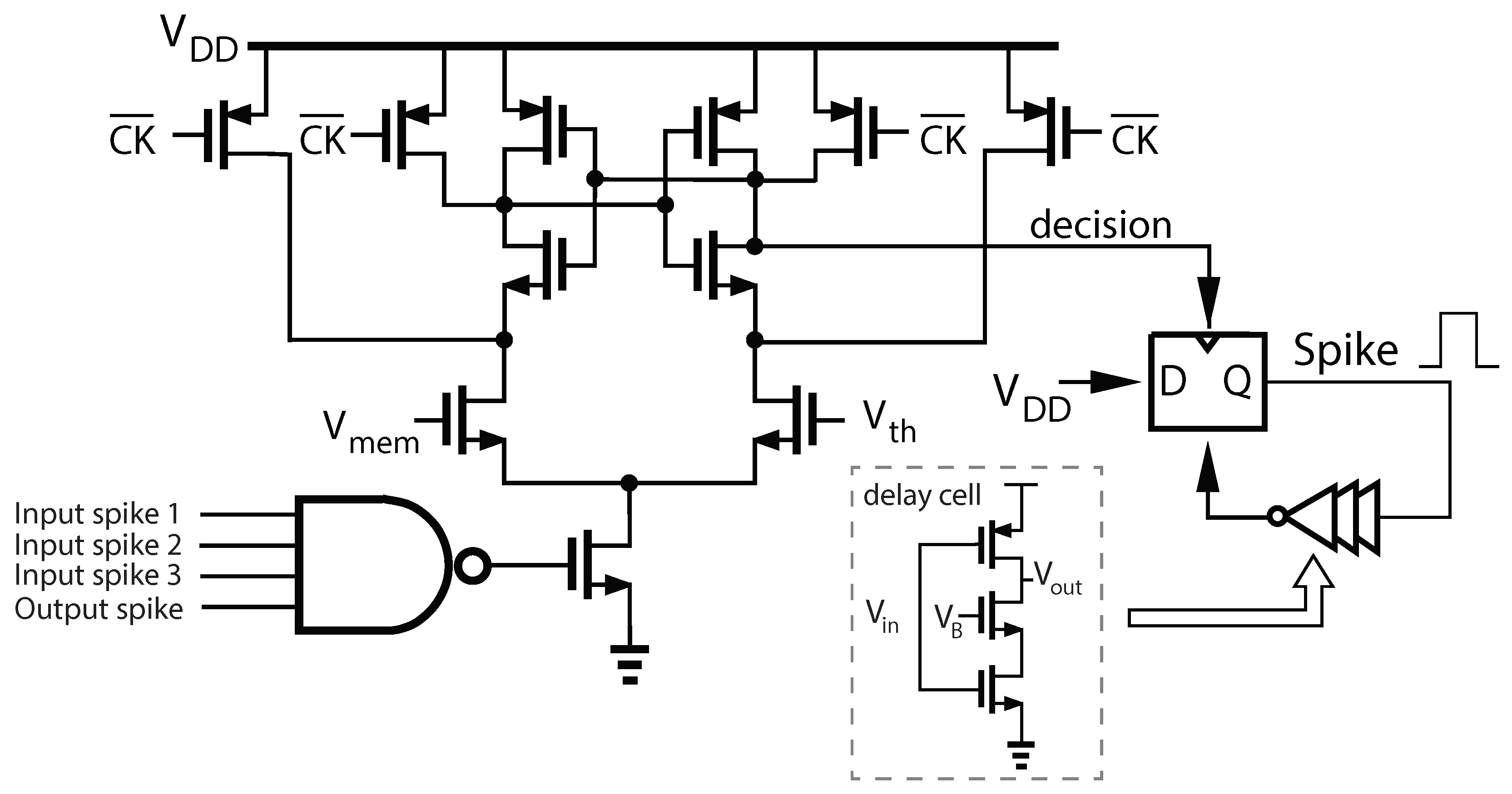
The goal of this work is to develop a low-power CMOS chip architecture that implements neuromodulatory tuning. In addition to presenting the neuromodulatory tuning algorithm and exploring its performance, we also present a complete neuron design to implements this algorithm on analog CMOS hardware.
Figure 7 shows the layout of the proposed neuron implementing NT fine tuning. The entire neuron, synapse and weight storage occupies only 598 μm 2 , with the neuron core (including membrane capacitor) occupying only 132 nm 2 . We have validated the simulation results from Section 6.1 using post-layout simulations in Cadence Virtuoso to model an XOR task using spiking neurons. Two neurons were chosen to be the inputs to the XOR “gate” and another designated as the output. A train of 10 spikes to an input neuron constituted a “1”. No input spikes constituted a “0”. The spikes propagated through the network according to the trained weights. The output was “0” if less than three spikes were observed at the output, otherwise the output was a “1”. The analog simulation showed 2 spikes at the output for a 0, and 4 for a 1.
The proposed neuron achieves performance competitive with the state-of-the-art in standalone neuron circuits (see Table 9). The total power for the neuron core varies with spike rate. Figure 7 shows the distribution of power for two spike rates and Figure 8 shows the energy/spike vs. spike rate.

7. Conclusions

Low-power analog machine learning has the potential to revolutionize multiple disciplines, but only if novel and physically-implementable learning algorithms are developed that enable in situ behavior modification on physical analog hardware. This paper presents a novel task transfer algorithm, termed neuromodulatory tuning, for machine learning based on biologically-inspired principles. On image recognition tasks, neuromodulatory tuning performs on test cases as well as traditional fine-tuning methods while requiring four orders of magnitude fewer active training parameters (although the total number of weights is comparable between methods). We verify this result using both deep forward networks and spiking neural network architectures. We also present a circuit design for a neuron that immplements neuromodulatory tuning, a potential layout for the use of such neurons on an analog chip, and a post-layout verification of its capabilities.
Neuromodulatory tuning has the advantage of being well-suited for implementation on neuromorphic hardware, enabling circuit implementations that support life-long learning for applications that require energy-efficient adaptation to constantly changing conditions, such as robotics, unmanned air vehicle guidance, and prosthetic limb controllers. Future research in this area should focus on probing the performance of NT in domains beyond image recognition; exploring the possibility of paired bias links in which multiple neurons connect to a single power domain region; and designing improved SNN update algorithms with stronger convergence properties.

Author Contributions

Neural network studies and writing, H.Y. and K.R.; circuit design, simulation, and writing, T.B.; problem conception, supervision, and writing—review and editing, N.F., S.-h.W.C., J.Y. and K.F.W. All authors have read and agreed to the published version of the manuscript.

Funding

This research received no external funding.

Data Availability Statement

The training data sets used in this study are widely available online.

Conflicts of Interest

The authors declare no conflict of interest.

References

  1. Pfeiffer, M.; Pfeil, T. Deep learning with spiking neurons: Opportunities and challenges. Front. Neurosci. 2018, 12, 774. [Google Scholar] [CrossRef] [PubMed] [Green Version]
  2. Voelker, A.R.; Rasmussen, D.; Eliasmith, C. A spike in performance: Training hybrid-spiking neural networks with quantized activation functions. arXiv 2020, arXiv:2002.03553. [Google Scholar]
  3. Ghosh-Dastidar, S.; Adeli, H. Spiking neural networks. Int. J. Neural Syst. 2009, 19, 295–308. [Google Scholar] [CrossRef] [PubMed] [Green Version]
  4. Tavanaei, A.; Ghodrati, M.; Kheradpisheh, S.R.; Masquelier, T.; Maida, A. Deep learning in spiking neural networks. Neural Networks 2019, 111, 47–63. [Google Scholar] [CrossRef] [PubMed] [Green Version]
  5. Ponulak, F.; Kasinski, A. Introduction to spiking neural networks: Information processing, learning and applications. Acta Neurobiol. Exp. 2011, 71, 409–433. [Google Scholar]
  6. Daumé III, H. Frustratingly Easy Domain Adaptation. In Proceedings of the 45th Annual Meeting of the Association of Computational Linguistics; Association for Computational Linguistics: Prague, Czech Republic, 2007; pp. 256–263. [Google Scholar]
  7. Sun, B.; Feng, J.; Saenko, K. Return of Frustratingly Easy Domain Adaptation. In Proceedings of the Thirtieth AAAI Conference on Artificial Intelligence; AAAI Press: Palo Alto, CA, USA, 2016; pp. 2058–2065. [Google Scholar]
  8. Blitzer, J.; McDonald, R.; Pereira, F. Domain Adaptation with Structural Correspondence Learning. In Proceedings of the 2006 Conference on Empirical Methods in Natural Language Processing; Association for Computational Linguistics: Sydney, Australia, 2006; pp. 120–128. [Google Scholar]
  9. Motiian, S.; Jones, Q.; Iranmanesh, S.; Doretto, G. Few-Shot Adversarial Domain Adaptation. In Proceedings of the Advances in Neural Information Processing Systems; Guyon, I., Luxburg, U.V., Bengio, S., Wallach, H., Fergus, R., Vishwanathan, S., Garnett, R., Eds.; Curran Associates, Inc.: New York, NY, USA, 2017; Volume 30. [Google Scholar]
  10. Liu, H.; Wang, J.; Long, M. Cycle Self-Training for Domain Adaptation. In Proceedings of the Advances in Neural Information Processing Systems; Ranzato, M., Beygelzimer, A., Dauphin, Y., Liang, P., Vaughan, J.W., Eds.; Curran Associates, Inc.: New York, NY, USA, 2021; Volume 34, pp. 22968–22981. [Google Scholar]
  11. Stojanov, P.; Li, Z.; Gong, M.; Cai, R.; Carbonell, J.; Zhang, K. Domain Adaptation with Invariant Representation Learning: What Transformations to Learn? In Proceedings of the Advances in Neural Information Processing Systems; Ranzato, M., Beygelzimer, A., Dauphin, Y., Liang, P., Vaughan, J.W., Eds.; Curran Associates, Inc.: New York, NY, USA, 2021; Volume 34, pp. 24791–24803. [Google Scholar]
  12. Lawrence, N.D.; Platt, J.C. Learning to learn with the informative vector machine. In Proceedings of the Ttwenty-First International Conference on Machine Learning, Banff, AB, Canada, 4–8 July 2004; p. 65. [Google Scholar]
  13. Raina, R.; Battle, A.; Lee, H.; Packer, B.; Ng, A.Y. Self-taught learning: Transfer learning from unlabeled data. In Proceedings of the 24th International Conference on Machine Learning, New York, NY, USA, 20–24 June 2007; pp. 759–766. [Google Scholar]
  14. Argyriou, A.; Evgeniou, T.; Pontil, M. Multi-task feature learning. Adv. Neural Inf. Process. Syst. 2006, 19, 1–2. [Google Scholar]
  15. Lee, S.I.; Chatalbashev, V.; Vickrey, D.; Koller, D. Learning a meta-level prior for feature relevance from multiple related tasks. In Proceedings of the 24th International Conference on Machine Learning, Corvalis, OR, USA, 20–24 June 2007; pp. 489–496. [Google Scholar]
  16. Li, D.; Zhang, H. Improved Regularization and Robustness for Fine-tuning in Neural Networks. In Proceedings of the Advances in Neural Information Processing Systems; Ranzato, M., Beygelzimer, A., Dauphin, Y., Liang, P., Vaughan, J.W., Eds.; Curran Associates, Inc.: New York, NY, USA, 2021; Volume 34, pp. 27249–27262. [Google Scholar]
  17. Dong, X.; Luu, A.T.; Lin, M.; Yan, S.; Zhang, H. How Should Pre-Trained Language Models Be Fine-Tuned Towards Adversarial Robustness? In Proceedings of the Advances in Neural Information Processing Systems; Ranzato, M., Beygelzimer, A., Dauphin, Y., Liang, P., Vaughan, J.W., Eds.; Curran Associates, Inc.: New York, NY, USA, 2021; Volume 34, pp. 4356–4369. [Google Scholar]
  18. Zhang, Y.; Hooi, B.; Hu, D.; Liang, J.; Feng, J. Unleashing the Power of Contrastive Self-Supervised Visual Models via Contrast-Regularized Fine-Tuning. In Proceedings of the Advances in Neural Information Processing Systems; Ranzato, M., Beygelzimer, A., Dauphin, Y., Liang, P., Vaughan, J.W., Eds.; Curran Associates, Inc.: New York, NY, USA, 2021; Volume 34, pp. 29848–29860. [Google Scholar]
  19. Vinyals, O.; Blundell, C.; Lillicrap, T.; Wierstra, D. Matching networks for one shot learning. Adv. Neural Inf. Process. Syst. 2016, 29, 1–2. [Google Scholar]
  20. Snell, J.; Swersky, K.; Zemel, R. Prototypical networks for few-shot learning. Adv. Neural Inf. Process. Syst. 2017, 30, 1–2. [Google Scholar]
  21. Brown, T.; Mann, B.; Ryder, N.; Subbiah, M.; Kaplan, J.D.; Dhariwal, P.; Neelakantan, A.; Shyam, P.; Sastry, G.; Askell, A.; et al. Language Models are Few-Shot Learners. In Proceedings of the Advances in Neural Information Processing Systems; Larochelle, H., Ranzato, M., Hadsell, R., Balcan, M., Lin, H., Eds.; Curran Associates, Inc.: New York, NY, USA, 2020; Volume 33, pp. 1877–1901. [Google Scholar]
  22. Yue, Z.; Zhang, H.; Sun, Q.; Hua, X.S. Interventional Few-Shot Learning. In Proceedings of the Advances in Neural Information Processing Systems; Larochelle, H., Ranzato, M., Hadsell, R., Balcan, M., Lin, H., Eds.; Curran Associates, Inc.: New York, NY, USA, 2020; Volume 33, pp. 2734–2746. [Google Scholar]
  23. Brown, Z.; Robinson, N.; Wingate, D.; Fulda, N. Towards neural programming interfaces. Adv. Neural Inf. Process. Syst. 2020, 33, 17416–17428. [Google Scholar]
  24. Agostinelli, F.; Hoffman, M.; Sadowski, P.; Baldi, P. Learning activation functions to improve deep neural networks. arXiv 2014, arXiv:1412.6830. [Google Scholar]
  25. Zaken, E.B.; Ravfogel, S.; Goldberg, Y. BitFit: Simple Parameter-efficient Fine-tuning for Transformer-based Masked Language-models, 2021. arXiv 2021, arXiv:2106.10199. [Google Scholar] [CrossRef]
  26. Kendall, J.; Pantone, R.; Manickavasagam, K.; Bengio, Y.; Scellier, B. Training end-to-end analog neural networks with equilibrium propagation. arXiv 2020, arXiv:2006.01981. [Google Scholar]
  27. Furber, S.B.; Galluppi, F.; Temple, S.; Plana, L.A. The SpiNNaker Project. Proc. IEEE 2014, 102, 652–665. [Google Scholar] [CrossRef]
  28. Voutsas, K.; Adamy, J. A Biologically Inspired Spiking Neural Network for Sound Source Lateralization. IEEE Trans. Neural Netw. 2007, 18, 1785–1799. [Google Scholar] [CrossRef] [PubMed]
  29. Yang, Z.; Han, Z.; Huang, Y.; Ye, T.T. 55nm CMOS Analog Circuit Implementation of LIF and STDP Functions for Low-Power SNNs. In Proceedings of the 2021 IEEE/ACM International Symposium on Low Power Electronics and Design (ISLPED), Virtual, 26–28 July 2021; pp. 1–6. [Google Scholar] [CrossRef]
  30. Rueckauer, B.; Liu, S.C. Conversion of analog to spiking neural networks using sparse temporal coding. In Proceedings of the 2018 IEEE International Symposium on Circuits and Systems (ISCAS), Florence, Italy, 27–30 May 2018; pp. 1–5. [Google Scholar] [CrossRef]
  31. Zhang, W.; Li, P. Spike-Train Level Backpropagation for Training Deep Recurrent Spiking Neural Networks. In Proceedings of the Advances in Neural Information Processing Systems; Wallach, H., Larochelle, H., Beygelzimer, A., d’Alché-Buc, F., Fox, E., Garnett, R., Eds.; Curran Associates, Inc.: New York, NY, USA, 2019; Volume 32. [Google Scholar]
  32. Miquel, J.R.; Tolu, S.; Schöller, F.E.T.; Galeazzi, R. RetinaNet Object Detector Based on Analog-to-Spiking Neural Network Conversion. In Proceedings of the 2021 8th International Conference on Soft Computing Machine Intelligence (ISCMI), Cairo, Egypt, 26–27 November 2021; pp. 201–205. [Google Scholar] [CrossRef]
  33. Ding, J.; Yu, Z.; Tian, Y.; Huang, T. Optimal ANN-SNN Conversion for Fast and Accurate Inference in Deep Spiking Neural Networks. arXiv 2021, arXiv:2105.11654. [Google Scholar]
  34. Li, Y.; Deng, S.; Dong, X.; Gu, S. Converting Artificial Neural Networks to Spiking Neural Networks via Parameter Calibration, 2022. arXiv 2022, arXiv:2205.10121. [Google Scholar] [CrossRef]
  35. Indiveri, G.; Chicca, E.; Douglas, R. A VLSI array of low-power spiking neurons and bistable synapses with spike-timing dependent plasticity. IEEE Trans. Neural Netw. 2006, 17, 211–221. [Google Scholar] [CrossRef] [Green Version]
  36. Han, B.; Srinivasan, G.; Roy, K. RMP-SNN: Residual Membrane Potential Neuron for Enabling Deeper High-Accuracy and Low-Latency Spiking Neural Network. In Proceedings of the 2020 IEEE/CVF Conference on Computer Vision and Pattern Recognition (CVPR), Seattle, WA, USA, 13–19 June 2020; pp. 13555–13564. [Google Scholar] [CrossRef]
  37. Li, J.; Zhao, C.; Hamedani, K.; Yi, Y. Analog hardware implementation of spike-based delayed feedback reservoir computing system. In Proceedings of the 2017 International Joint Conference on Neural Networks (IJCNN), Anchorage, AK, USA, 14–19 May 2017; pp. 3439–3446. [Google Scholar] [CrossRef]
  38. Nitundil, S.; Susi, G.; Maestú, F. Design of an Analog Multi-Neuronal Spike-sequence Detector (MNSD) based on a 180nm CMOS Leaky Integrate amp; Fire with Latency Neuron. In Proceedings of the 2021 International Conference on Advances in Electrical, Computing, Communication and Sustainable Technologies (ICAECT), Bhilai, India, 19–20 February 2021; pp. 1–6. [Google Scholar] [CrossRef]
  39. Sun, Q.; Schwartz, F.; Michel, J.; Herve, Y.; Dal Molin, R. Implementation Study of an Analog Spiking Neural Network for Assisting Cardiac Delay Prediction in a Cardiac Resynchronization Therapy Device. IEEE Trans. Neural Netw. 2011, 22, 858–869. [Google Scholar] [CrossRef]
  40. Mostafa, H. Supervised Learning Based on Temporal Coding in Spiking Neural Networks. IEEE Trans. Neural Netw. Learn. Syst. 2018, 29, 3227–3235. [Google Scholar] [CrossRef] [Green Version]
  41. Hsieh, H.Y.; Tang, K.T. VLSI Implementation of a Bio-Inspired Olfactory Spiking Neural Network. IEEE Trans. Neural Netw. Learn. Syst. 2012, 23, 1065–1073. [Google Scholar] [CrossRef]
  42. Kim, M.H.; Hwang, S.; Bang, S.; Kim, T.H.; Lee, D.K.; Ansari, M.H.R.; Cho, S.; Park, B.G. A More Hardware-Oriented Spiking Neural Network Based on Leading Memory Technology and Its Application with Reinforcement Learning. IEEE Trans. Electron. Devices 2021, 68, 4411–4417. [Google Scholar] [CrossRef]
  43. Cincon, V.; Vatajelu, E.I.; Anghel, L.; Galy, P. From 1.8 V to 0.19 V voltage bias on analog spiking neuron in 28 nm UTBB FD-SOI technology. In Proceedings of the 2020 Joint International EUROSOI Workshop and International Conference on Ultimate Integration on Silicon (EUROSOI-ULIS), Caen, France, 1–30 September 2020; pp. 1–4. [Google Scholar] [CrossRef]
  44. Danneville, F.; Sourikopoulos, I.; Hedayat, S.; Loyez, C.; Hoël, V.; Cappy, A. Ultra low power analog design and technology for artificial neurons. In Proceedings of the 2017 IEEE Bipolar/BiCMOS Circuits and Technology Meeting (BCTM), Miami, FL, USA, 19–21 October 2017; pp. 1–8. [Google Scholar] [CrossRef]
  45. Satyaraj, I.; Kailath, B.J. A simple PSTDP circuit for Analog Implementation of Spiking Neural Networks. In Proceedings of the 2020 IEEE 4th Conference on Information Communication Technology (CICT), Chennai, India, 3–5 December 2020; pp. 1–4. [Google Scholar] [CrossRef]
  46. Kim, D.; She, X.; Rahman, N.M.; Chekuri, V.C.K.; Mukhopadhyay, S. Processing-In-Memory-Based On-Chip Learning With Spike-Time-Dependent Plasticity in 65-nm CMOS. IEEE Solid-State Circuits Lett. 2020, 3, 278–281. [Google Scholar] [CrossRef]
  47. Azghadi, M.R.; Al-Sarawi, S.; Iannella, N.; Abbott, D. Efficient design of triplet based Spike-Timing Dependent Plasticity. In Proceedings of the the 2012 International Joint Conference on Neural Networks (IJCNN), Brisbane, Australia, 10–15 June 2012; pp. 1–7. [Google Scholar] [CrossRef] [Green Version]
  48. Clements, J. Transmitter timecourse in the synaptic cleft: Its role in central synaptic function. Trends Neurosci. 1996, 19, 163–171. [Google Scholar] [CrossRef]
  49. Agnati, L.F.; Zoli, M.; Strömberg, I.; Fuxe, K. Intercellular communication in the brain: Wiring versus volume transmission. Neuroscience 1995, 69, 711–726. [Google Scholar] [CrossRef]
  50. Yorgason, J.T.; Zeppenfeld, D.M.; Williams, J.T. Cholinergic Interneurons Underlie Spontaneous Dopamine Release in Nucleus Accumbens. J. Neurosci. 2017, 37, 2086–2096. [Google Scholar] [CrossRef] [PubMed] [Green Version]
  51. Beaulieu, J.; Gainetdinov, R.R. The physiology, signaling, and pharmacology of dopamine receptors. Pharmacol. Rev. 2011, 63, 182–217. [Google Scholar] [CrossRef] [PubMed] [Green Version]
  52. Depue, R.A.; Collins, P.F. Neurobiology of the structure of personality: Dopamine, facilitation of incentive motivation, and extraversion. Behav. Brain Sci. 1999, 22, 491–517. [Google Scholar] [CrossRef]
  53. Frank, M.J. Dynamic dopamine modulation in the basal ganglia: A neurocomputational account of cognitive deficits in medicated and nonmedicated Parkinsonism. J. Cogn. Neurosci. 2005, 17, 51–72. [Google Scholar] [CrossRef] [Green Version]
  54. Stoof, J.C.; Kebabian, J.W. Two dopamine receptors: Biochemistry, physiology and pharmacology. Life Sci. 1984, 35, 2281–2296. [Google Scholar] [CrossRef]
  55. Reiner, A.; Levitz, J. Glutamatergic Signaling in the Central Nervous System: Ionotropic and Metabotropic Receptors in Concert. Neuron 2018, 98, 1080–1098. [Google Scholar] [CrossRef] [Green Version]
  56. ImageNet Dataset. Available online: https://www.image-net.org/ (accessed on 2 May 2022).
  57. Coates, A.; Ng, A.; Lee, H. An analysis of single-layer networks in unsupervised feature learning. In Proceedings of the Fourteenth International Conference on Artificial Intelligence and Statistics, JMLR Workshop and Conference Proceedings, Fort Lauderdale, FL, USA, 11–13 April 2011; pp. 215–223. [Google Scholar]
  58. Food Image Dataset. Available online: https://www.epfl.ch/labs/mmspg/downloads/food-image-datasets/ (accessed on 2 May 2022).
  59. Blood Cell Images. 2018. Available online: https://www.kaggle.com/datasets/paultimothymooney/blood-cells (accessed on 2 May 2022).
  60. Liu, X.; Chi, M.; Zhang, Y.; Qin, Y. Classifying High Resolution Remote Sensing Images by Fine-Tuned VGG Deep Networks. In Proceedings of the IGARSS 2018—2018 IEEE International Geoscience and Remote Sensing Symposium, Valencia, Spain, 22–27 July 2018; pp. 7137–7140. [Google Scholar] [CrossRef]
  61. Nagaraju, Y.; Venkatesh; Swetha, S.; Stalin, S. Apple and Grape Leaf Diseases Classification using Transfer Learning via Fine-tuned Classifier. In Proceedings of the 2020 IEEE International Conference on Machine Learning and Applied Network Technologies (ICMLANT), Hyderabad, India, 20–21 December 2020; pp. 1–6. [Google Scholar] [CrossRef]
  62. Kandel, I.; Castelli, M. The effect of batch size on the generalizability of the convolutional neural networks on a histopathology dataset. ICT Express 2020, 6, 312–315. [Google Scholar] [CrossRef]
  63. Aamir, S.A.A.; Stradmann, Y.; Müller, P.; Pehle, C.; Hartel, A.; Grübl, A.; Schemmel, J.; Meier, K. An Accelerated LIF Neuronal Network Array for a Large-Scale Mixed-Signal Neuromorphic Architecture; IEEE Transactions on Circuits and Systems I: Regular Papers; IEEE: Piscataway, NJ, USA, 2018. [Google Scholar]
Figure 1. Depiction of neuromodulatory tuning (NT) in contrast with traditional fine-tuning (TFT). In NT, the weights of the pre-trained network are frozen, preserving all learned feature information pertaining to the original training task. A set of auxiliary bias neurons with randomly initialized weights is then inserted into the network, and the auxiliary bias weights are then updated in response to the new learning task. In this diagram, color indicates the weights’ update status: red for active, blue for frozen. NT requires far fewer parameter updates than traditional fine-tuning methods, although loss information must still be propagated backward through the entire network.
Jlpea 12 00059 g001
Figure 2. Representation of the Spiking Neural Network (SNN) experimental setup. In these experiments we construct a SNN that mimics the function and purpose of the traditional pretrained VGG-19 classifier layers. To accomplish this, we pass data from a dataset d, where d = {STL-10, Food-11, BCCD}, through the feature layers of VGG-19 to generate a feature embedding for a particular data instance. A traditional usage of VGG-19, like in Section 4, would then pass the feature embedding through the fully-connected classifier layers to produce a model prediction. In these experiments, however, we pass the feature embedding through spiking classifier layers which then in turn produce a spiking model prediction.
Jlpea 12 00059 g002
Figure 3. Schematic diagram of the proposed leaky integrate-and-fire neuron with NT ( V D D , v a r i a b l e ) capabilities. The Up and Down signals are generated from the input spike and weight signals.
Jlpea 12 00059 g003
Figure 4. Neuron outputs with the same input spike pattern and synaptic weights, but with varied bias weights implemented as (a) V D D = 550 mV and (b) V D D = 750 mV.
Jlpea 12 00059 g004
Figure 5. Schematic of the threshold comparator with dynamic clocking, and tunable spike generator circuit.
Jlpea 12 00059 g005
Figure 6. Schematic of (a) a one-directional pseudo-resistor and its asymmetric resistance characteristic and (b) the proposed pseudo-resistor showing symmetric resistance characteristics.
Jlpea 12 00059 g006
Figure 7. The distribution of power within the neuron core.
Jlpea 12 00059 g007
Figure 8. The energy/spike decreases as V D D increases. This is because a higher V D D yields a higher synapse current and therefore more output spikes for the same number of input spikes.
Jlpea 12 00059 g008
Table 1. Validation accuracy on STL-10, Food-11, and BCCD datasets after 5 epochs, mean of five training runs using learning rate (lr) = {0.01} and and using the full training set for each dataset after being balanced.
STL-10 accFood-11 accBCCD acc
additive bias tuning0.10000.08630.2498
multiplicative neuromodulatory tuning0.84470.71100.3966
Table 2. Validation accuracy on the STL-10, Food-11, and BCCD dataset after 10 epochs, mean of five training runs using learning rate (lr) = {0.1, 0.01, 0.001, 0.0001} and using the full training set for each dataset after being balanced. N T 1 = additional bias implementation, N T 2 = modify existing bias implementation. Highest average accuracies are bolded.
STL-10 accFood-11 accBCCD acc
N T 1 (lr = 0.1)0.82370.68190.3864
N T 2 (lr = 0.1)0.76260.53090.3280
N T 1 (lr = 0.01)0.84910.71840.4126
N T 2 (lr = 0.01)0.84200.70300.3800
N T 1 (lr = 0.001)0.84290.69290.3986
N T 2 (lr = 0.001)0.85170.71730.4234
N T 1 (lr = 0.0001)0.78560.59460.3939
N T 2 (lr = 0.0001)0.83330.66310.4008
N T 1 —average0.82530.67200.3979
N T 2 —average0.82240.65360.3831
Table 3. Validation accuracy on the STL-10, Food-11, and BCCD datasets after 10 epochs, mean of five training runs using learning rate (lr) = {0.1, 0.01, 0.001, 0.0001, 0.00001} and using the full training set for each dataset after being balanced. Highest average accuracies and highest best-performing accuracies are bolded.
STL-10 acc (n = 500)Food-11 acc (n = 280)BCCD acc (n = 2400)
N T 1 (lr = 0.1)0.82370.68190.3864
TFT (lr = 0.1)0.10310.08760.2487
N T 1 (lr = 0.01)0.84910.71840.4126
TFT (lr = 0.01)0.15400.09870.2496
N T 1 (lr = 0.001)0.84290.69290.3986
TFT (lr = 0.001)0.86170.71840.2509
N T 1 (lr = 0.0001)0.78560.59460.3939
TFT (lr = 0.0001)0.88360.80600.4291
N T 1 (lr = 0.00001)0.49690.22180.3484
TFT (lr = 0.00001)0.87240.73870.4209
N T 1 —average0.75960.58190.3880
TFT—average0.57500.48990.3198
N T 1 —best0.84910.71840.4126
TFT—best0.88360.80600.4291
N T 1 —tuned parameters43,29044,29137,284
TFT—tuned parameters123,652,866123,653,867123,646,860
Table 4. Validation accuracy on the Food-11 dataset after 10 epochs, mean of ten training runs using bath sizes (bs) = {16, 32, 64, 128}, and using the full training set for the Food-11 dataset after being balanced. The batch size 128 is too large for the TFT setup and is thus omitted. The best learning rates for TFT and N T 1 methods were determined from preliminary results.
acc (bs = 16)acc (bs = 32)acc (bs = 64)acc (bs = 128)
N T 1 (lr = 0.01)0.69240.68610.69330.7162
TFT (lr = 0.0001)0.79000.80680.8118-
Table 5. A repeat of the experiments sin Table 3, but with a large subset of neuromodulatory inputs removed. Validation accuracy on the STL-10, Food-11, and BCCD datasets after 10 epochs, mean of five training runs using learning rate (lr) = {0.01, 0.0001} and using the full training set for each dataset after being balanced. The best learning rates for TFT and N T 1 methods were determined from results in Table 3.
STL-10 acc (n = 500)Food-11 acc (n = 280)BCCD acc (n = 2400)
N T 1 (lr = 0.01)0.82130.70560.3680
TFT (lr = 0.0001)0.88360.80600.4291
N T 1 —tuned parameters18,20219,20312,196
TFT—tuned parameters123,652,866123,653,867123,646,860
Table 6. Validation accuracy on the Food-11 dataset on SNN after 10 epochs, mean of 10 training runs using bath sizes (bs) = {16, 32, 64, 128}.
acc (bs = 16)acc (bs = 32)acc (bs = 64)acc (bs = 128)
N T 1 (lr = 0.1)0.45680.46050.45700.4647
TFT (lr = 0.1)0.13040.12430.11450.0770
Table 7. Validation accuracy on STL-10, Food-11, and the BCCD dataset in a spiking neural network (SNN) architecture. Models were trained for 50 epochs for STL-10, Food11, and the BCCD dataset, respectively. Average of five training runs. Best per-task performance of neuromodulatory tuning ( N T 2 ) and traditional fine-tuning (TFT), respectively, is underlined. N T 2 refers to the modify existing bias implementation of NT and N T 1 refers to the additional bias implementation described in Section 3.2.
lr 0.0001lr 0.001lr 0.01lr 0.1
no tuning0.00070.00070.00070.0007
TFT0.88880.80140.25820.1274
STL-10 N T 2 0.00000.00000.30520.3062
N T 1 0.00000.00090.54280.5731
additive bias0.00100.00080.00060.0025
no tuning0.03410.03410.03410.0341
TFT0.01470.07290.10170.1168
Food-11 N T 2 0.00630.36450.45370.4615
N T 1 0.00200.36780.45640.4665
additive bias 0.0840 0.1864 0.1404 0.1414
no tuning0.00050.00050.00050.0005
TFT0.10030.25080.25070.2508
BCCD N T 2 0.25010.25090.13710.0680
N T 1 0.25080.25090.20410.0591
additive bias0.18480.21370.21440.2505
Table 8. Validation accuracy and parameter on STL-10, Food-11, and the BCCD dataset in a spiking neural network (SNN) architecture. Models were trained for 50 epochs for STL-10, Food11, and the BCCD dataset, respectively. Accuracy from the learning rate with best average accuracy of five training runs. N T 2 refers to the modify existing bias implementation of NT and N T 1 refers to the additional bias implementation described in Section 3.2.
Best AccuracyParameter Amount
TFT0.8888123,642,856
STL-10 N T 2 0.30629192
N T 1 0.57319192
additive bias0.00259192
TFT0.0356123,653,867
Food-11 N T 2 0.461520,203
N T 1 0.466520,203
additive bias 0.1864 20,203
TFT0.2508123,646,860
BCCD N T 2 0.250913,196
N T 1 0.250913,196
additive bias0.250513,196
Table 9. Comparison of our proposed neuron implementing neuromodulatory tuning with the state of the art in standalone neurons. * Total area includes neuron core, synapse, and weight storage.
This WorkJoubert et al., 2012Cruz-Albrecht et al., 2012Rangan et al., 2010Jayawan 2008
Process (nm)28659090350
Area μm 2 598 (Total *) 132 (Core)5384428972800
Max f s p i k e (Hz)3.3 M1.9 M1007 k1 M
Energy/spike (pJ)1.08410.419
Publisher’s Note: MDPI stays neutral with regard to jurisdictional claims in published maps and institutional affiliations.

