Article

Implementing a Timing Error-Resilient and Energy-Efficient Near-Threshold Hardware Accelerator for Deep Neural Network Inference

Bridge Lab, Electrical and Computer Engineering, Utah State University, Logan, UT 84321, USA
*
Author to whom correspondence should be addressed.
J. Low Power Electron. Appl. 2022, 12(2), 32; https://doi.org/10.3390/jlpea12020032
Submission received: 16 November 2021 / Revised: 19 April 2022 / Accepted: 23 May 2022 / Published: 6 June 2022
(This article belongs to the Special Issue Hardware for Machine Learning)

Abstract

:
Increasing processing requirements in the Artificial Intelligence (AI) realm has led to the emergence of domain-specific architectures for Deep Neural Network (DNN) applications. Tensor Processing Unit (TPU), a DNN accelerator by Google, has emerged as a front runner outclassing its contemporaries, CPUs and GPUs, in performance by 15×–30×. TPUs have been deployed in Google data centers to cater to the performance demands. However, a TPU’s performance enhancement is accompanied by a mammoth power consumption. In the pursuit of lowering the energy utilization, this paper proposes PREDITOR—a low-power TPU operating in the Near-Threshold Computing (NTC) realm. PREDITOR uses mathematical analysis to mitigate the undetectable timing errors by boosting the voltage of the selective multiplier-and-accumulator units at specific intervals to enhance the performance of the NTC TPU, thereby ensuring a high inference accuracy at low voltage. PREDITOR offers up to 3×–5× improved performance in comparison to the leading-edge error mitigation schemes with a minor loss in accuracy.

1. Introduction

Rapid progress in the Artificial Intelligence (AI) realm has evidenced an emergence in the domain-specific AI architectures to sustain the colossal boom in the development of Deep Neural Network (DNN) applications. The rising efficiency of DNN accelerators further bears witness to the ongoing empirical advancements within the sphere of Deep Learning [1,2]. Google’s Tensor Processing Unit (TPU), a systolic array of multiplier-and-accumulate (MAC) units, has been spearheading this race by demonstrating a massive performance boost over the contemporary CPUs and GPUs [3].
However, the growth in AI processing is accompanied by a monumental increase in the power consumption as affirmed by the carbon footprint for a single AI training [4]. To sustain the performance and trim the energy consumption, we conceive operating TPU in the Near-Threshold Computing (NTC) realm. Operating a TPU at NTC benefits in a massive energy savings as the operating voltage is scaled close to the threshold voltage. However, extreme Process Variation (PV) sensitivity [5] introduced at NTC induces a high rate of timing errors, which degrades the overall system performance [6], thereby reducing the energy-efficiency gains at low-voltage operation [7]. In this paper, we emphasize the significance of undetectable timing errors (Section 2.1) on the performance of an NTC TPU and exploit the architectural homogeneity to detect and tackle timing errors, thereby presenting a reliable and energy-efficient TPU design paradigm.
Razor is a very popular timing speculation methodology using a double sampling flip-flop to detect and correct timing errors [8]. Razor employs an instruction replay to correct the erroneous computation. The tightly pipelined architecture of the TPU will result in inflating the execution time, thereby restricting the use of an instruction replay in a TPU. TE-Drop, a recently proposed technique, prompts the MAC unit encountering a timing error to steal a clock cycle from the downstream MAC to correct the timing error [9]. The erring MAC overrides the downstream MAC’s output with its corrected value. However, TE-Drop does not address the timing errors, which cannot be detected by Razor Flip-Flop [8] which leads to the erroneous value to propagate down the output.
To overcome the limitations in existing schemes, we propose a novel timing error prediction strategy based on the foreseeable timing error occurrence pattern in the TPU systolic array. We observe the impacts of undetectable timing errors on the inference accuracy (Section 2.1). Integrating the mathematical analysis on the initially recorded timing error data and using an efficient voltage-boosting mechanism, we propose PREDITOR—a novel low-power error-resilient TPU design paradigm to predict and mitigate timing errors. To the best of our knowledge, this is the first work emphasizing the impacts of undetectable timing errors on the inference accuracy and presents a channel to limit its effects. The following are the precise contributions in this paper:
  • We observe a monumental increase of undetected timing errors at higher frequencies and ultra-low NTC voltages (Section 2).
  • We propose PREDITOR—a low-power TPU design paradigm that predicts and mitigates the timing errors over a range of operational cycles using an effective voltage boost mechanism (Section 3).
  • We demonstrate that PREDITOR tackles up to ∼ 68 % of the undetectable timing errors, thereby preserving the inference accuracy of the DNN datasets. PREDITOR offers 3×–5× better performance in comparison to TE-DROP and Modified Razor Flip-Flop, with under 3% average loss in accuracy for five out of eight DNN datasets and incurs an area and power overhead of ∼ 7.7 % and ∼ 2.5 % , respectively (Section 5).
  • We illustrate that PREDITOR offers up to 87 % energy-efficiency gain in relative to a TPU operating in the Super-Threshold Computing (STC) realm, while utilizing only 14 % of its power (Section 5).

2. Motivation

In this section, we investigate the correlation between the data flow and timing error emergence, and we reveal the concealed opportunity that can be utilized to tackle timing errors in a TPU systolic array. Section 2.1 provides the background of a TPU and elaborates the drawbacks for an NTC TPU operation. Section 2.2 introduces the architectural homogeneity of the TPU. Using the cross-layer methodology explained in Section 2.3, we explore the timing error profiles illustrated in Section 2.4 and establish the need for a timing error prediction scheme in an NTC TPU.

2.1. Background and Limitations

2.1.1. Systolic Array Based DNN Accelerator

DNNs use multiple layers of computation to obtain the output inference. In each layer, the activation matrix is multiplied with the weight matrix. TPU employs a systolic array of 256 × 256 MAC units to accelerate matrix multiplication [3]. The activation matrix and weight matrix both maintain an 8-bit precision. The weight matrices are pre-loaded into the MACs, while the activation flows from left to right in successive clock cycles. The 24-bit precision accumulator output from each MAC moves downstream in each cycle.

2.1.2. Limitations to NTC Performance

Dynamic Scaling of Voltage (DVS) is a common practice used in the modern processing elements to yield significant power savings. The critical voltage is fixed at an optimum point to ensure correct operation of the processing element. However, aggressive scaling leads to an increase in the critical path due to the decrease in the clock period of the operation.
Figure 1a shows the typical scenario of an operation. The critical path is shorter than the clock period of an operation. In Figure 1b, the frequency of the operation has increased to obtain better performance. During this scenario, the clock period of an operation decreases, leading to the delayed transitioning of the data (i.e., data1 to data2.). This phenomenon where the wrong data (i.e., data1.) are being latched onto the output instead of the correct data (i.e., data2.) is called a timing error [5,10]. Timing speculation methods such as Razor uses a double sampling flop to capture this delayed transitioning in data and employs an instant replay to latch the correct data onto the output [8]. Figure 1c depicts the operation of a Razor flop, where a delayed clock is employed by the shadow flop to detect the delayed transition. However, when the frequency of operation increases even further, the speculative window becomes too small even for the Razor flop to capture the delayed transition. Figure 1d elaborates the scenario when the delayed transitions cannot be captured any further. These extremely delayed transitions are the undetectable timing errors.
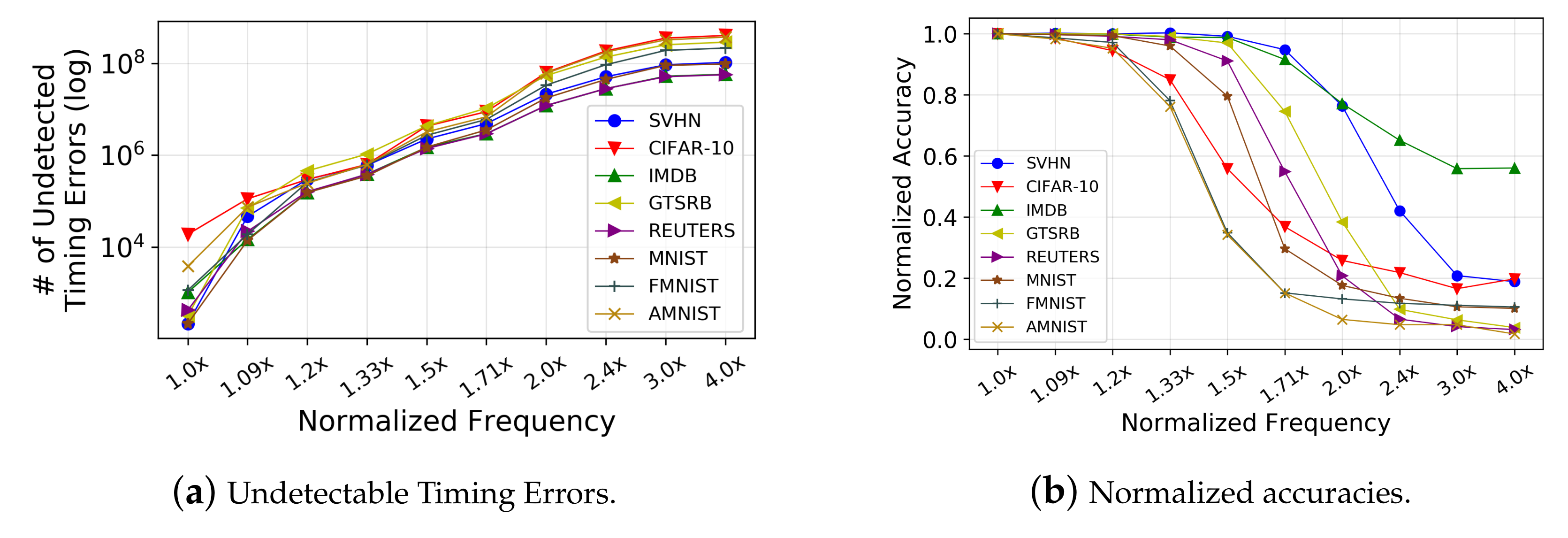
Figure 2a depicts the increase of the undetectable timing errors with an increase of frequency for eight different DNN datasets. These undetectable errors propagate down the systolic array, resulting in an erroneous output, adversely affecting the system performance [6,7]. Figure 2b appropriately shows the drop in inferential accuracy as the operational frequency level is bolstered [9]. Especially, in case of DNN computations, where inference accuracy dictates the performance of the system, the deterioration of classification accuracy renders the system inept to address the increasing performance needs.

2.2. Predictive Systolic Array Dataflow

There exists a strong interdependence between the data flow pattern inside the systolic array and number of timing errors occurring during the systolic array operation. Although the occurrence of timing errors are majorly dependent on the computational delays, the magnitude of timing errors per cycle of operation is dependent on the number of operations during the same period of clock cycles. Due to the disparate number of operations during every active execution cycle, the scope of timing errors varies but closely follows a foreseeable pattern. To further investigate this property, we employ an exhaustive cross-layer methodology, which is discussed next.

2.3. Methodology

We synthesize a MAC unit at NTC, using 15 nm FinFET library from NanGate  [11]. To model the PV at NTC for FinFET, we use VARIUS-NTV models [12]. For a conservative estimate, we consider PV-induced delays in randomly chosen 2% of the gates in the circuit. We use our in-house Statistical Timing Analysis (STA) tool to investigate the delay distribution of the sensitized path for different inputs to the MAC unit. We use our in-house TPU systolic array simulator to simulate the working of a TPU. We use different levels of high degree timing error inducing input vectors with our TPU simulator to investigate the operational flow and timing error intricacies.

2.4. Results and Significance

Figure 3 demonstrates the extensively observed timing error count variances in a systolic array operation. The Y-axes are normalized to the highest timing error in the respective plots. X-axes are normalized to the total number of operational cycles. Plots1–3 in Figure 3 show an exponential increase/decrease in the timing errors, and Plot 4 depicts a relatively linear rise/fall. The operational cycle in which the highest timing errors occur varies across the plots in Figure 3. For example, in Plot 2 of Figure 3, the highest timing error occurs at the 42nd cycle, whereas for Plot 3, the highest timing error occurs at the 58th cycle.
The results indicate a disparity in the timing error profiles, but all the plots have a symmetrical nature. Plots 1–3 of Figure 3 nearly exhibit a normal distribution curve characteristic, while Plot 4 resembles a triangular curve. The symmetrical nature of the profiles is mainly attributed to the uneven number of MAC units being active during each clock cycle of a systolic array operation. Utilizing this predictable timing error occurrence model, we devise a prediction strategy to significantly lower the timing errors in a TPU. With this insight, we propose our scheme—PREDITOR, to mitigate up to 68% of the timing errors by boosting the operating voltage during the high timing error occurrence cycles.

3. Design

In this section, we propose Analytical PREDIcTion based ErrOR Resilient TPU (PREDITOR), a novel low-power design paradigm to enhance the error resilience of an NTC TPU using mathematical analysis of the detectable timing errors. Section 3.1 outlines the design overview. Section 3.2, Section 3.3 and Section 3.4 elaborate on the components of PREDITOR.

3.1. Design Overview

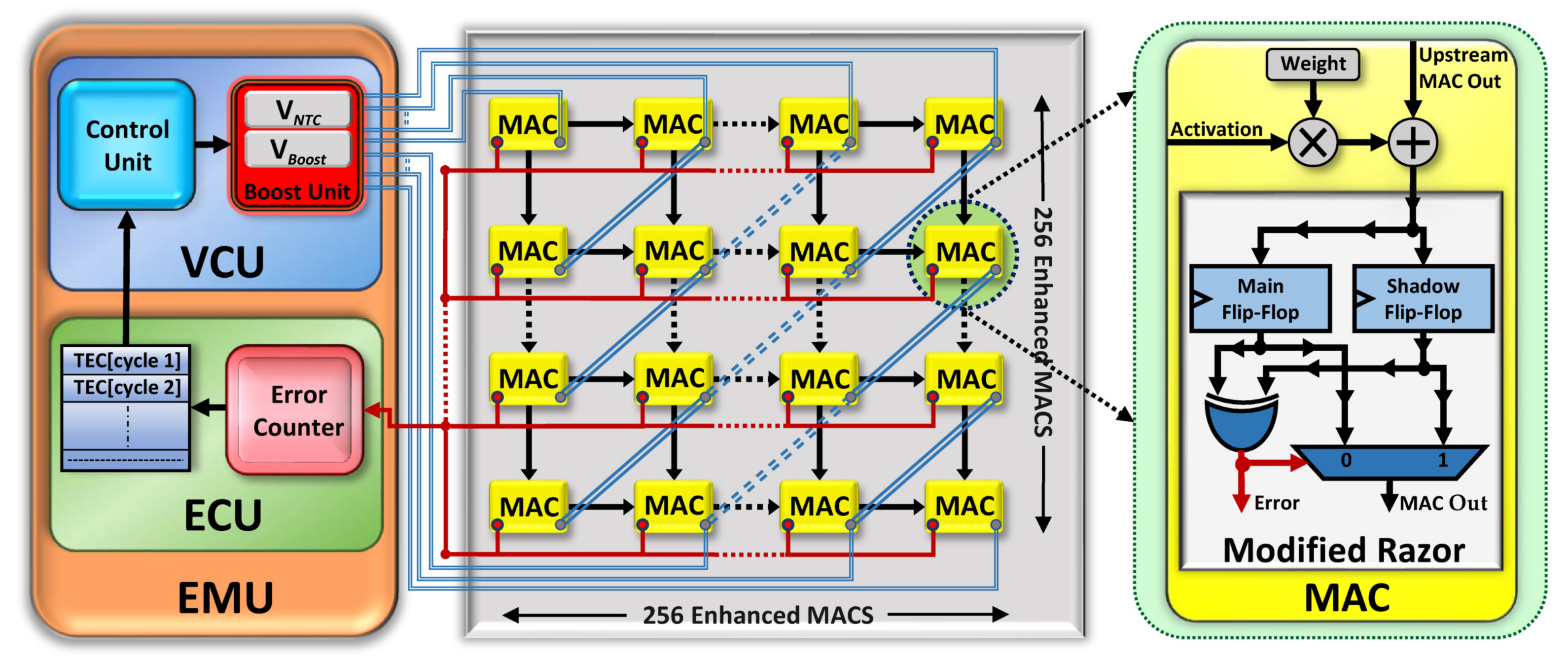
Figure 4 depicts the top-level overview of PREDITOR. The prime enhancement of PREDITOR is the Error Management Unit (EMU). The main components of an EMU are Error Collection Unit (ECU) and Voltage Control Unit (VCU). Each MAC unit is augmented with a Modified Razor Flip-Flop (MRFF) to detect and mitigate timing errors during the non-boosted cycles of operation. MRFF captures a timing error using a shadow latch and delivers an error signal to the ECU. Additionally, MRFF also provides the corrected value to the downstream MAC unit. ECU records the number of timing errors occurring during every operational clock cycle. VCU profiles and analyzes the timing error information from ECU once every two clock cycles to predict the operational clock cycle intervals, which yields maximum timing errors. VCU will then boost the operating voltage of the MACs during the predicted intervals to ensure an error-free operation. Since the data flow in the systolic array as a diagonal wavefront, MACs along the diagonal (i.e., left bottom to right top) will be active/inactive at the same time [3]. Hence, VCU will only boost the voltage of the MACs which are computationally active, thereby introducing a minuscule energy overhead.

3.2. Modified Razor Flip-Flop (MRFF)

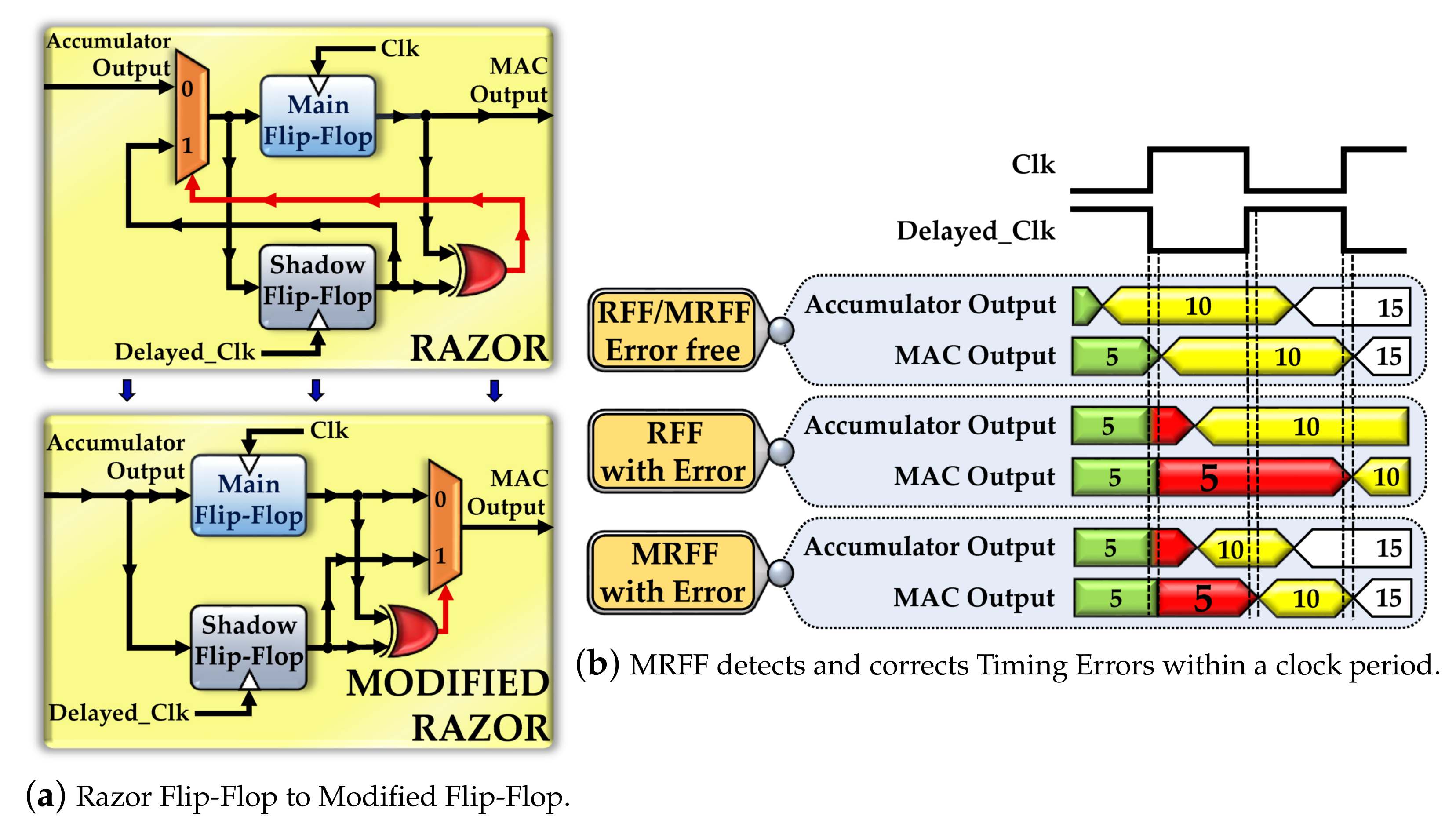
MRFF detects and corrects timing errors without using any additional operational clock cycles. In a MAC unit, a multiplier is sensitized only to the periodically changing activation input, as the pre-loaded weights remain unchanged throughout the entire systolic array operation. Additionally, the multiplier operation is computationally prolonged compared to the accumulation operation. It thus opens up a timing aperture, which can be exploited to override the previously transmitted erroneous value with the updated upstream MAC output. Figure 5a depicts the changes in the schematic between a regular Razor Flip-Flop (RFF) and MRFF.
Figure 5b demonstrates the error-handling capabilities of an RFF and MRFF for a column-wise systolic array operation. As depicted in Figure 5b, whenever an RFF detects a timing error due to the delayed manipulation of the output data, an instant replay is initiated, which requires an additional clock cycle to correct the erroneous value. However, an MRFF will detect and correct the timing error within the same clock cycle by opportunistically using the timing aperture.
However, MRFF cannot correct timing errors when the computational delays are beyond detection (Section 2.1.2). Hence, VCU will utilize the timing error information stored in ECU to predict the range of operational cycles to mitigate timing errors, which is explained in Section 3.4.

3.3. Error Collection Unit (ECU)

ECU contains a 16-bit Error Counter and a content-addressable memory. During each operational clock cycle, ECU captures the timing errors from individual MAC units, and these error signals are accumulated using the 16-bit Error Counter. The Timing Error Count (TEC) (i.e., the total number of timing errors) obtained during every clock cycle is stored in the consecutive locations of a content-addressable memory and successively updated at the end of every operational clock cycle.

3.4. Voltage Control Unit (VCU)

VCU houses the Control Unit (CU) and the Boost Unit (BU). CU computes the range of operational clock cycles for voltage boosting by analyzing the cycle-wise TEC from ECU. BU boosts the supply voltage of MACs for the clock cycle interval predicted by the CU. Voltage boosting aids in mitigating both detectable and undetectable timing errors.

3.4.1. Control Unit (CU)

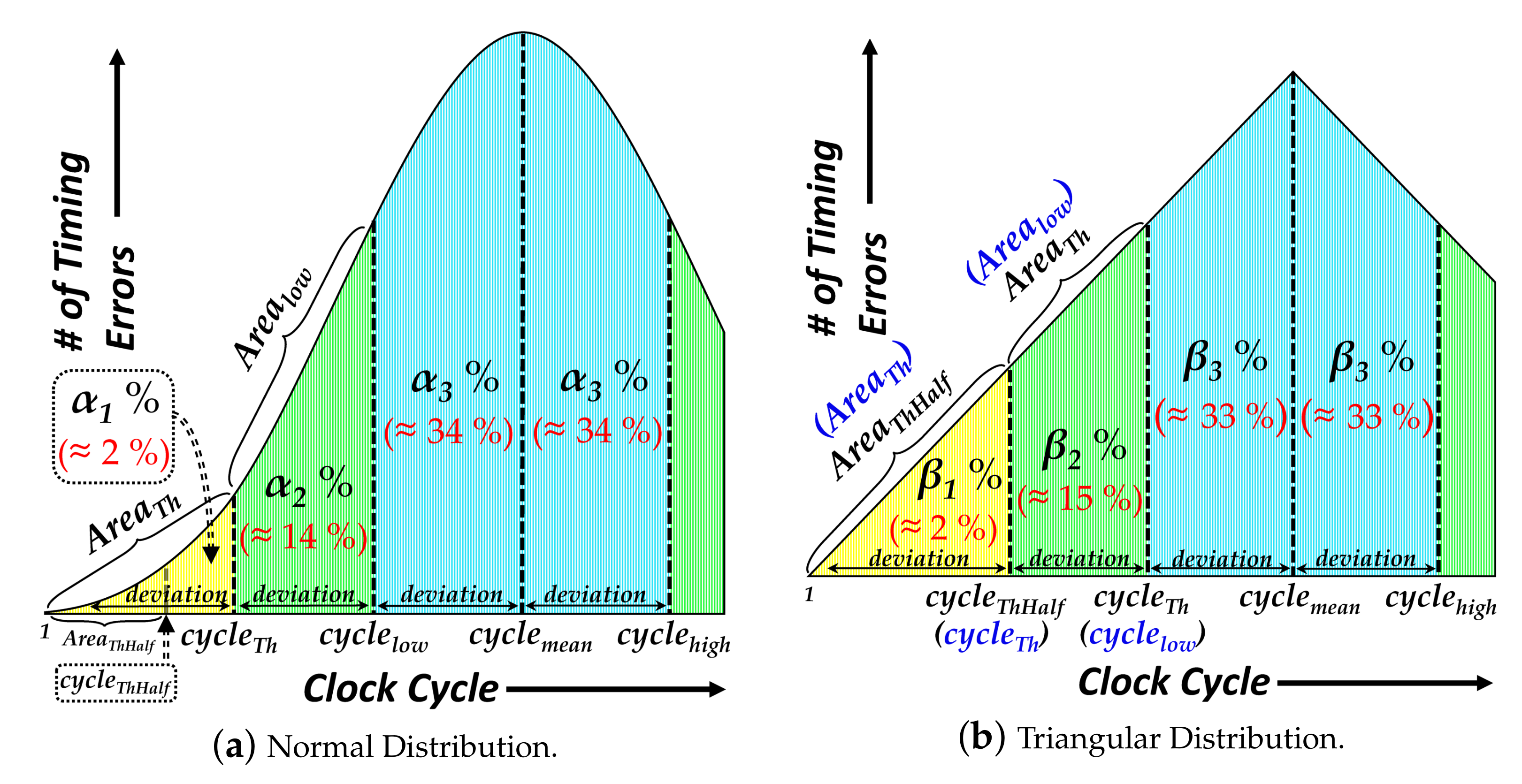
CU is responsible for predicting the operational clock cycle intervals yielding maximum timing errors. Based on the findings in Section 2.4, we develop an algorithm modeled on the Normal Distribution Curve characteristic. Since ∼ 68 % of the area of a Normal Distribution curve is covered between the first standard deviations from the mean, by mathematical analysis, we identify that ∼ 68 % of the timing errors will be occurring within the ∼ 33 % operational clock cycles centered around the mean clock cycle. Hence, we target ∼ 68 % of undetectable timing errors to be mitigated by PREDITOR.
Figure 6a,b show the representative area-wise Normal and Triangular Distribution of a timing error profile. The boost cycles prediction procedures are elaborated in Algorithm 1. Based on experimental analysis, we determine that a rapid rise in the rate of timing errors results in the timing error profile exhibiting a Normal Distribution curve characteristic, and a slower rise results in a Triangular Distribution curve characteristic. Hence, we define a metric, Curve Factor (CF), to determine the nature of the timing error profile. CF is defined as the ratio of Areas between the Threshold clock cycle ( c y c l e T h ) and Half Threshold clock cycle ( c y c l e T h H a l f ) (line 18 of Algorithm 1) (Figure 6a). The values of c y c l e T h and c y c l e T h H a l f are empirically ascertained based on earlier analysis.
Figure 6. Representative Timing Error Profiles.
Jlpea 12 00032 g006
Algorithm 1: Boost Cycles Prediction Algorithm
1:
d i m s y s t o l i c _ a r r a y _ d i m e n s i o n
2:
c y c l e o p s c u r r e n t _ o p e r a t i o n a l _ c l o c k _ c y c l e
3:
t o t a l _ n u m _ c y c l e s ( ( 3 * d i m ) 2 )
4:
c y c l e m e a n ( t o t a l _ n u m _ c y c l e s ÷ 2 )
5:
c y c l e h i g h ( 4 / 3 ) c y c l e m e a n
6:
c y c l e l o w ( 2 / 3 ) c y c l e m e a n
7:
c y c l e T h ( 1 / 3 ) c y c l e m e a n
8:
c y c l e T h H a l f ( 1 / 2 ) c y c l e T h  
9:
procedureArea_Calculation( i n i t _ c y c l e , f i n a l _ c y c l e )
10:
     A r e a 0
11:
    for  i t e r a t o r ( i n i t _ c y c l e ) t o ( f i n a l _ c y c l e )  do
12:
         A r e a A r e a + T E C [ i t e r a t o r ]
13:
    end for
14:
    return A r e a
15:
end procedure 
16:
procedureCurve_Prediction( c y c l e o p s )
17:
    if  ( c y c l e o p s = c y c l e T h )  then
18:
         C F A r e a T h / A r e a T h H a l f
19:
        if  C F > N D t h r e s h  then
20:
            C u r v e _ D i s t c o e f f N D c o e f f
21:
            b o o s t _ i n i t i a t e 1
22:
        else if  C F < N D t h r e s h & C F > T D t h r e s h  then
23:
            C u r v e _ D i s t c o e f f T D c o e f f
24:
            c y c l e l o w c y c l e T h
25:
            c y c l e T h c y c l e T h H a l f
26:
            b o o s t _ i n i t i a t e 1
27:
        else
28:
            b o o s t _ i n i t i a t e 0
29:
        end if
30:
    end if
31:
end procedure
32:
procedureBoost_Interval_Compute( c y c l e o p s )
33:
    if  c y c l e o p s = c y c l e l o w + 1  then
34:
        if  A r e a l o w < ( C u r v e _ D i s t c o e f f * A r e a T h )  then
35:
            c y c l e T h c y c l e T h + 1
36:
            c y c l e l o w c y c l e l o w + 1
37:
        else
38:
            d e v i a t i o n ( c y c l e l o w c y c l e T h )
39:
            c y c l e h i g h ( c y c l e l o w + ( 2 * d e v i a t i o n ) )
40:
        end if
41:
    end if
42:
end procedure
To predict the boost intervals, we compare the accumulated areas A r e a T h and A r e a l o w . Areas (i.e., summation of TECs) between specific cycles are computed using an area calculation heuristic (lines 9–15 of Algorithm 1). For example, A r e a l o w is a summation of TECs from c y c l e T h to c y c l e l o w . As new TECs are updated after every clock cycle, a balancing metric, C u r v e _ D i s t c o e f f , is used to dynamically balance the areas at specific clock cycle boundaries (i.e., c y c l e T h and c y c l e l o w .). The empirically determined balancing metric for a Normal Distribution curve ( N D c o e f f ) is expressed in Equation (1). The cycles are adjusted dynamically (lines 35–36 of Algorithm 1) in case the areas are unbalanced.
N D c o e f f = α 2 α 1
For a Triangular Distribution curve, appropriate changes for cycles under consideration are made (lines 23–25 of Algorithm 1), as the timing error counts at lower cycles need to be analyzed. The empirically determined balancing metric for a Triangular Distribution curve ( T D c o e f f ) is defined as:
T D c o e f f = β 2 β 1
A very low CF evades the need for voltage boosting (line 28 of Algorithm 1). Whenever there is alteration in the central cycle (Plot 3 of Figure 3), an increase in the timing error rate (not shown in Algorithm 1) is employed to dynamically calibrate the change.

3.4.2. Boost Unit (BU)

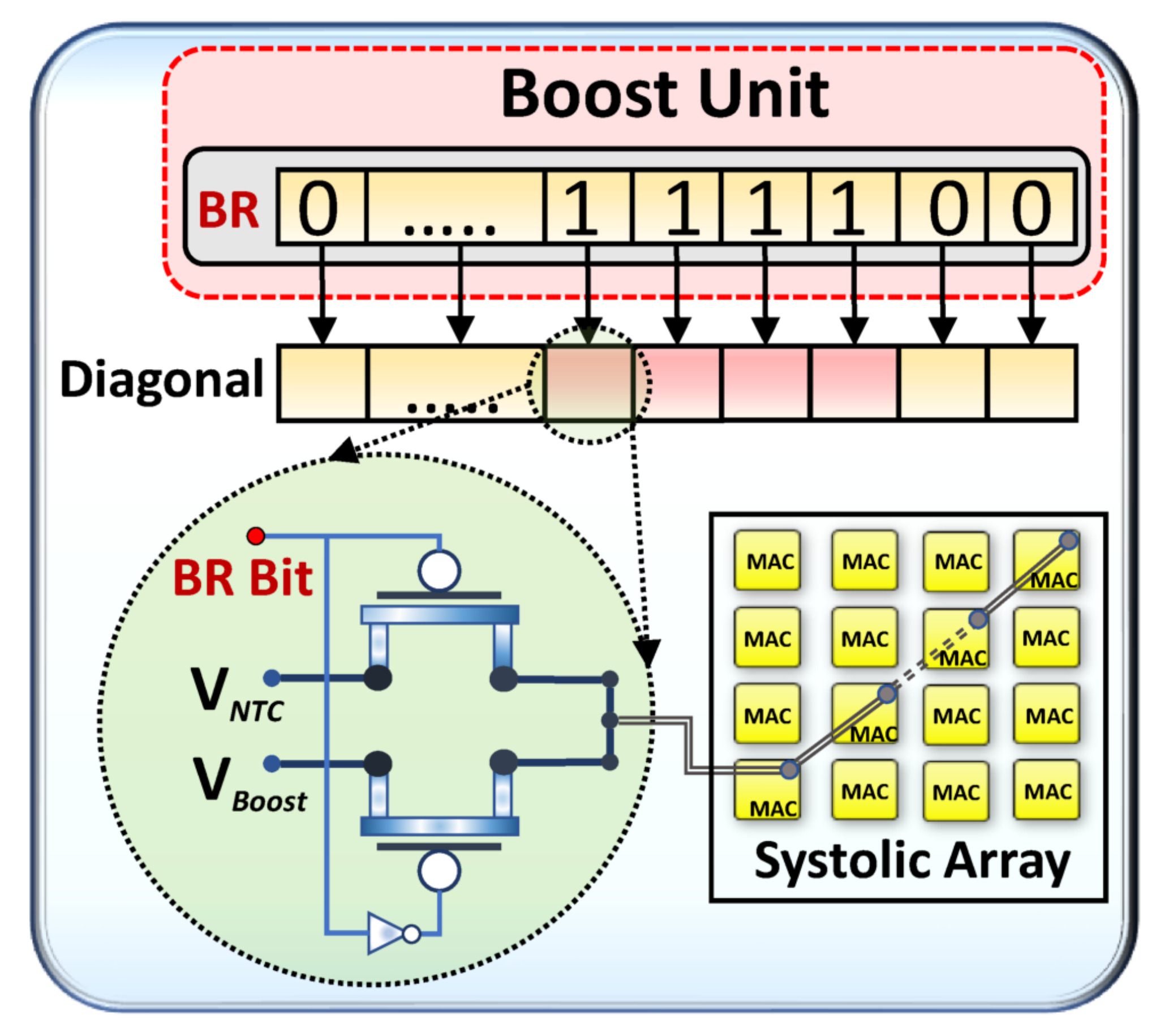
BU boosts the operating voltage of the MAC units to mitigate detectable and undetectable timing errors. As depicted in Figure 7, BU houses the Boost Register (BR), where each bit of this 511-bit register corresponds to a series of active MAC units along the diagonally active wavefront [13]. A boosting technique proposed in [14] is employed by BU, where supply voltage to MAC units has two rails, V N T C and V B o o s t . V N T C represents near-threshold voltage, which is set at 0.45 V, and V B o o s t is the boost voltage, which is set at 0.6 V. BU utilizes the procedure in Algorithm 3 to boost the supply voltage. Incorporating the booster infrastructure in [14], we observe that switching between V N T C and V B o o s t can be procured within a single cycle of operation. BU boosts the supply voltage to V B o o s t and switches to V N T C at the end of each boost cycle. To maintain a trade-off between boosting cycle intervals and the voltage boosting energy overhead, bits in BR are set empirically. This action is performed to lower the energy footprint in case the magnitude of timing errors is significantly high in number. In such a scenario, MRFF will continue to handle the detectable timing errors. The experimental results and area/power overheads are discussed in Section 5.
Figure 7. Interaction of BU with MACs along the diagonal.
Jlpea 12 00032 g007
Algorithm 2:Voltage Boost Algorithm
1:
procedureVoltage_Boost( c y c l e o p s , b o o s t _ i n i t i a t e )
2:
    if  b o o s t _ i n i t i a t e = 1  then
3:
        if  ( c y c l e o p s c y c l e l o w ) ( c y c l e o p s c y c l e h i g h )  then
4:
            s u p p l y _ v o l t a g e V B o o s t
5:
        else
6:
            s u p p l y _ v o l t a g e V N T C
7:
        end if
8:
    end if
9:
end procedure

4. Methodology

In this section, we describe our comprehensive cross-layer methodology, as shown in Figure 8, which is used to implement our proposed design. The cross-layer methodology will aid in evaluating our proposed design’s capabilities across DNN applications.

4.1. Device Layer

In order to estimate gate delay distributions, we simulate HSPICE models of basic logic gates (viz., NOR, NAND and Inverter) based on a 16 nm Predictive Technology Model. To incorporate the impact of PV at NTC, we consider the VARIUS-NTV model [10]. We model the impact of FinFETs using a VARIUS-TC model [15]. To affirm sensitized path delay in a MAC unit, the delays of basic gates are employed in the circuit layer (Section 4.2).

4.2. Circuit Layer

We implement a systolic array in the Verilog RTL description and enhance it with PREDITOR components. RTLs are synthesized using Synopsys Design Compiler to estimate area and power overheads. We obtain sensitized delays for a MAC array using our in-house STA tool by employing real dataset-driven inputs. By utilizing libraries of delay distributions for basic logic gates from HSPICE simulations (Section 4.1), the STA tool provides the delays of sensitized paths in the MAC circuit.

4.3. Architecture Layer

We employ our in-house cycle-accurate TPU systolic array simulator developed using C++ based on the TPU architectural details provided in [3]. To accurately model timing errors resembling real-time sensitized path delays in MAC units, we incorporate the STA tool (Section 4.2) into the TPU simulator. We replicate a real-life inference engine by interfacing Keras [16] with our TPU simulator. Using Keras and employing TensorFlow in the backend, we train multiple DNN applications, as mentioned in Section 5.3. Table 1 provides the size and layer information for the eight DNN datasets. We have used a filter size of (3,3) and default stride of 1 for all datasets. We have also added padding to the input feature map. The DNN datasets include representations from different Neural Network domains (Image Recognition, Speech, Audio, etc.). The diverse range of datasets aids in exploring the efficacy of PREDITOR in handling the timing violations, arising due to the wider set of variations in the activation patterns. The trained models have varying input sizes and utilize the state-of-art layers such as dropout and batch normalization. The trained model weights and the activations from each layer are extracted into 256 × 256 8-bit integer matrices. The TPU simulator performs the matrix multiplication operation for each pair of activation and weight matrices. The resulting output matrices are combined together to determine the inference accuracy.

5. Experimental Results

In this section, we evaluate the effectiveness of different timing error-resilient schemes by employing a TPU in NTC operating conditions. The baseline operation condition of the NTC TPU is (0.45V, 67.5MHz) to ensure error-free systolic array operations. Section 5.1 describes the different comparative schemes. Section 5.2 presents the error resilience of PREDITOR. Section 5.3 elaborates the inference accuracies. Section 5.4 presents the energy efficiency of PREDITOR. Section 5.5 discusses the area and power overheads.

5.1. Comparative Schemes

  • Baseline TPU (B-TPU): This technique does not employ any timing speculation methodologies and propagates the erroneous values down the systolic array computation stages [25].
  • TE-DROP (TED): In this scheme, an MAC encountering a timing error recomputes the correct value by borrowing a clock cycle from the downstream MAC. The downstream MAC effectively annuls its operation and procures the recomputed upstream MAC output onto the next stage [9].
  • MRFF: This scheme exploits the timing aperture to drive the delayed output onto the downstream MAC. Delayed output beyond detection results in an erroneous value being propagated down the systolic array.
  • PREDITOR (PRED): This is our proposed scheme which uses the timing error information obtained using the timing speculation mechanism to predict and mitigate eminent timing errors by boosting the operating voltage of the MAC units for a definite period of operation (Section 3).

5.2. Error Resilience

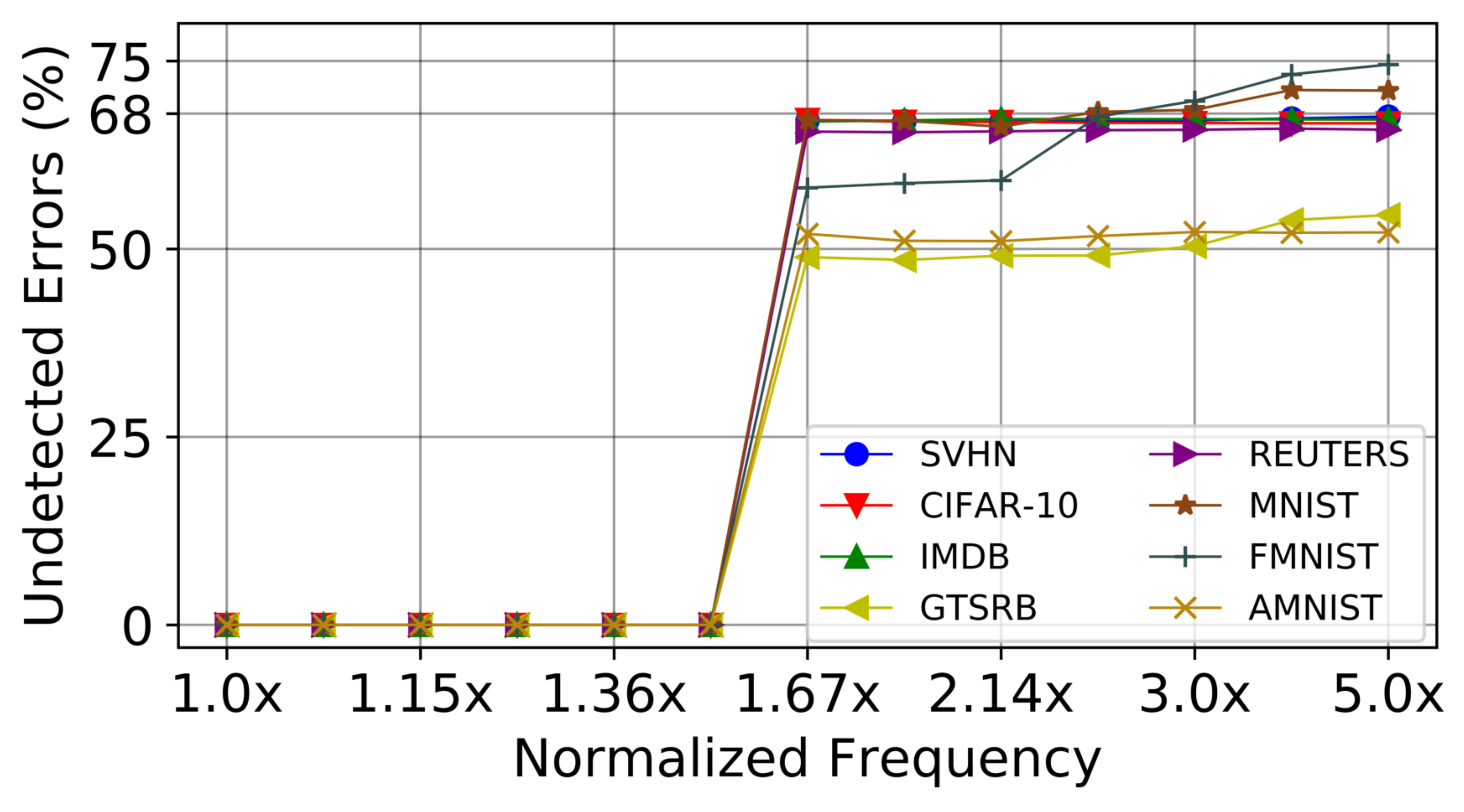
Figure 9 demonstrates the number of undetected timing errors mitigated by PREDITOR when the TPU is operated at higher frequencies compared to the baseline frequency of operation. The Y-axis represents the percentage of undetected timing errors effectively handled by PREDITOR. The operating voltage is kept constant at 0.45 V for all frequencies denoted by the X-axis. The X-axis is normalized to the baseline frequency of operation. Up to 1.44x, the baseline frequency and detectable timing errors are effectively handled by MRFF. Hence, the effect of timing errors on the inference accuracy is negligible, as explained in Section 5.3. PREDITOR’s voltage boosting mechanism becomes eminent after 1.44x the baseline frequency, thereby correcting the undetectable timing errors. Meanwhile, ∼ 68 % of undetectable timing errors are mitigated for six out of eight DNN datasets, as evidenced in Figure 9, validating the expectation elaborated in Section 3.4.1.

5.3. Inference Accuracy and Voltage Boost

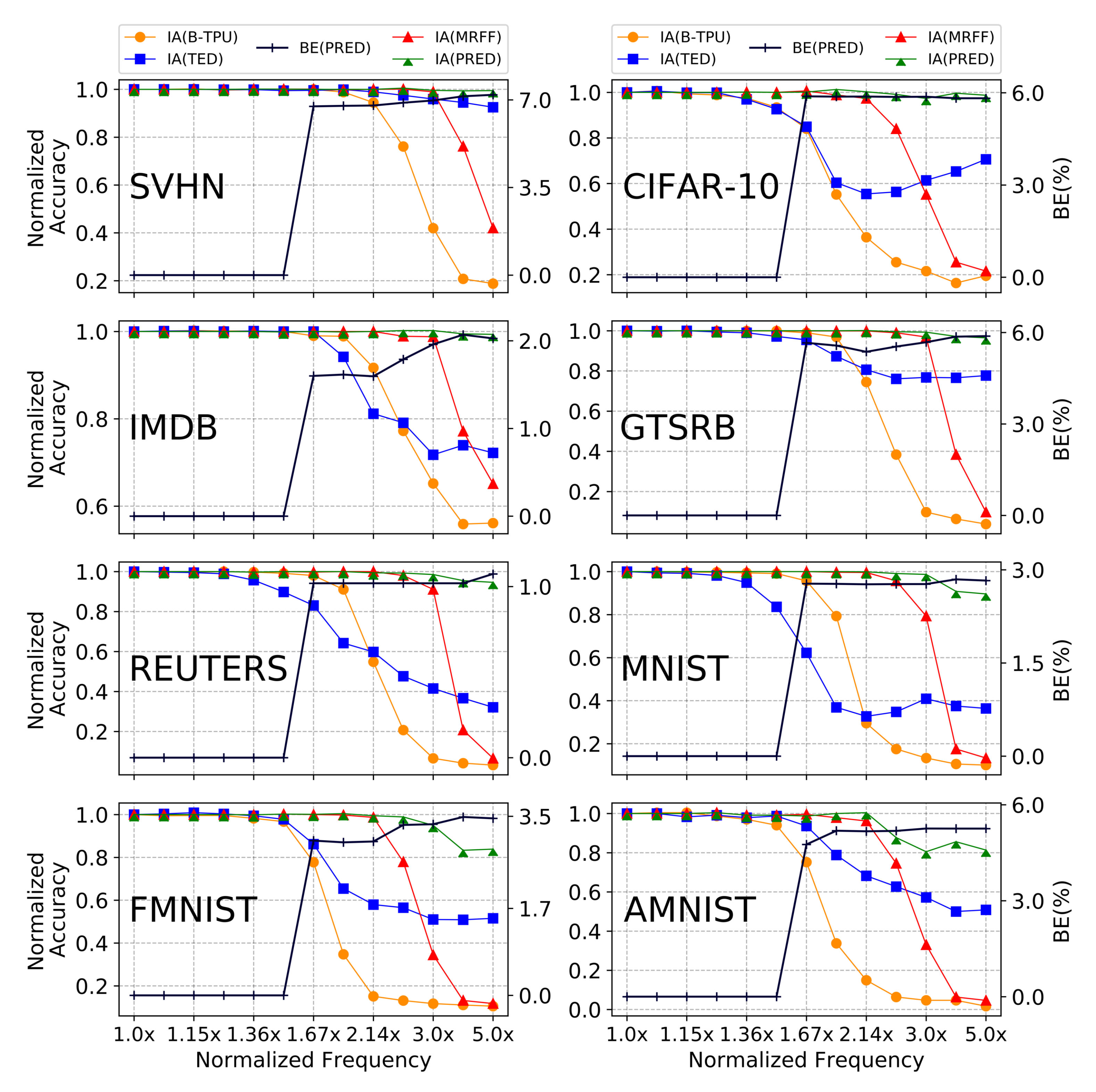
Figure 10 depicts the variations in normalized inference accuracies for eight different datasets with various error-resilient schemes. Y-axes are normalized to error-free inference accuracy at the baseline frequency for all datasets (error-free accuracy for datasets are SVHN: 0.94 [17], CIFAR-10: 0.77 [22], IMDB: 0.89 [20], GTSRB: 0.97 [18], REUTERS: 0.80 [19], MNIST: 0.98 [21], FMNIST: 0.89 [23], AMNIST: 0.92 [24])). Figure 10 also depicts the Voltage Boost Energy (BE) of PREDITOR across all frequencies of operation. BE is computed as the percentage of energy consumed by an NTC TPU operating at baseline conditions without any voltage-boosting mechanism.
Consistent error resiliency is provided by all schemes up to 1.36× the baseline frequency. As the performance is increased, PREDITOR surpasses B-TPU, TED and MRFF by providing an appreciably better accuracy. PREDITOR mitigates more timing errors at higher frequencies due to a superior prediction engine. The number of undetected timing errors during non-boosted cycles for AMNIST and FMNIST is relatively high, resulting in a drop of accuracy for PREDITOR. A large number of MAC operations being bypassed due to higher timing errors contributes to a deterioration of accuracy for TED. MRFF encounters a sudden fall in accuracy at higher frequencies due to an increase in undetected timing errors. Hence, PREDITOR-enhanced NTC TPU contributes to an accuracy loss of only 3 % in five datatsets when operated up to 5× the baseline frequency.
Voltage boosting from PREDITOR is not utilized until 1.67× the baseline frequency due to a lower number of timing errors which are corrected by MRFF. As frequency is scaled beyond 1.67×, nearly all datasets witness an identical rise in BE, as voltage boosting across a period of operational cycles becomes imminent. BE for four out of eight DNN datasets (SVHN, CIFAR-10, GTSRB and AMNIST) is relatively higher at ∼ 7 % , compared to other datasets, as the significant number of timing errors occurring during initial operational cycles compels PREDITOR’s prediction mechanism to boost a relatively higher number of operational cycles. However, the number of boosted cycles is relatively small compared to the entire systolic array of operation cycles.

5.4. Is NTC TPU Worth It?

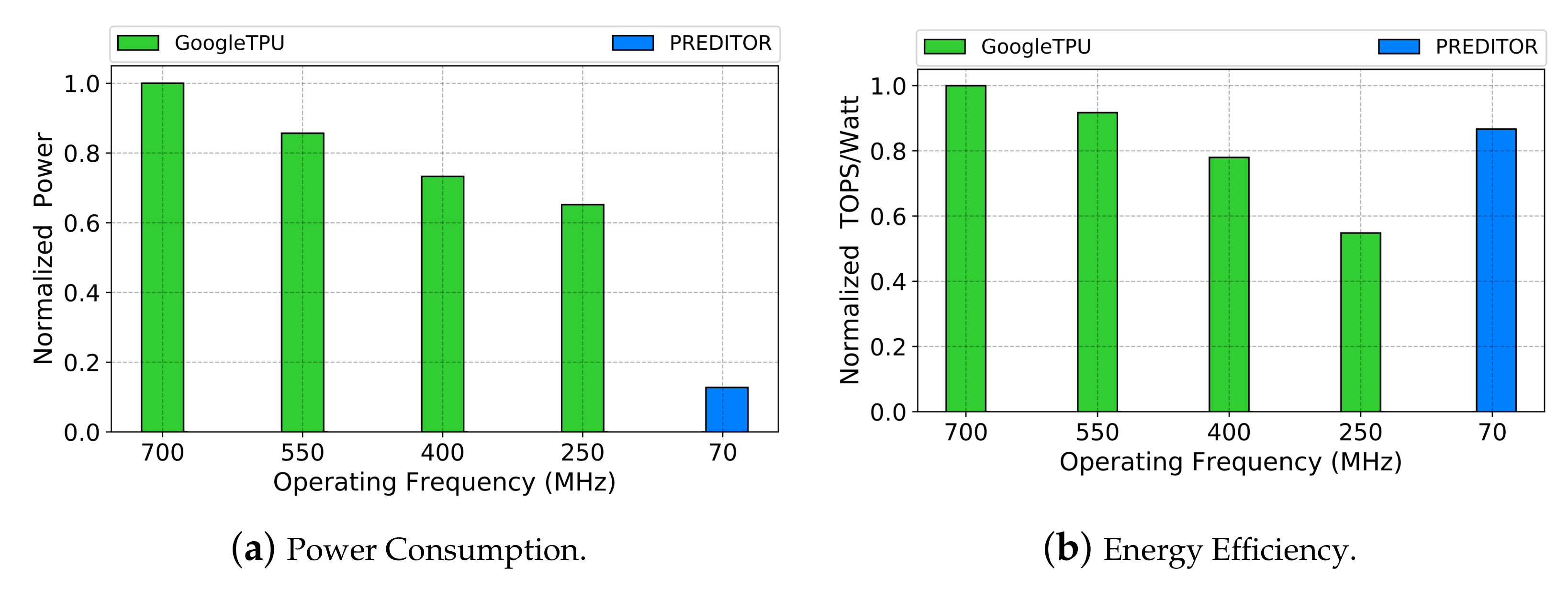
Figure 11 presents the average power consumption and energy efficiency, measured in Tera Operations Per Second (TOPS)/Watt of a GoogleTPU for 8 DNN datasets, as it scaled from the STC to NTC region. The figures also demonstrate the power consumption and energy efficiency of PREDITOR operating at NTC. Power consumption and TOPS/Watt metrics at different frequencies are normalized to that of the GoogleTPU operating at STC (i.e., 700 MHz). A steady decline in power is noted for GoogleTPU as the operating voltage is reduced along with the operating frequency. The power consumption of PREDITOR is significantly lower than GoogleTPU as it is operated in the NTC region. As the GoogleTPU is scaled below the STC region, timing errors appear in the system, leading to a deterioration in the performance [9]. However, an NTC TPU equipped with PREDITOR can effectively handle timing errors for more than 3× its baseline frequency (Section 5.2 and Section 5.3), thereby providing an efficient performance per unit consumption. PREDITOR working at NTC delivers up to 87 % energy-efficiency gain of a GoogleTPU operating at STC (Figure 11b), while consuming only 14 % of its power (Figure 11a). Hence, PREDITOR is validated as a low-power and error-resilient design paradigm, offering a high performance in an NTC TPU.

5.5. Hardware Overheads

The area and power overhead incurred by PREDITOR are ∼ 7.7 % and ∼ 2.5 % respectively. Area overhead in PREDITOR is due to inclusion of the MRFF into each MAC unit and EMU into the TPU systolic array. Power overheads obtained are in comparison to the error-free operation of a baseline NTC TPU.

6. Related Work

Earlier research efforts associated with our work focus on enhancing the energy efficiency and error resilience of DNN accelerators. Koppala et al. proposed a framework to improve the energy efficiency and performance of DNNs by retraining the DNN for an approximate DRAM device to increase the error tolerance of DNNs and meeting the DNN accuracy requirements by ensuring an approximate DRAM partition being efficiently mapped from a specific DNN data type [26]. Zhao et al. presented an algorithmic-based fault tolerance technique utilizing checksum schemes to ensure high detection and correction ability accompanied by a lower runtime overhead [27]. Ozen et al. obtained a highly resilient DNN using modified algorithms by comparing the reductions in the vulnerability surface through appropriate quantization techniques using efficient training methods [28]. Shafique et al. shed light on techniques to improve the performance and energy efficiency of Edge AI systems using optimizations in hardware/software and present cost-effective techniques to address the reliability threats [29]. Yu et al. proposed a hardware pruning technique which uses SIMD-aware weight and node pruning in coalition to enhance the energy efficiency of DNNs [30]. Ozen et al. filtered the effect of bit errors before the layer execution using a unique median feature selection to tackle high error rates [31]. Zhang et al. presented an aggressive voltage underscaling method without deteriorating the classification accuracy amidst the presence of high timing errors [9]. Ye et al. introduce a flexible framework with a hybrid convolution processing engine to implement a hybrid DNN accelerator with high performance [32]. Choi et al. achieved significant energy savings by using sensitive weight analysis to divide computations among MAC units [33]. Lin et al. introduced a statistical error compensation-based technique to correct timing errors occuring due to process variation while operating in near-threshold conditions [34]. Yu et al. proposed a hardware prunning technique which uses SIMD-aware weight and node prunning in coalition to reduce the size of underlying hardware at run time to enhance the energy efficiency of DNNs [30]. Zhang et al. presented an aggressive voltage underscaling method without deteriorating the classification accuracy amidst the presence of high timing errors [9]. Kim et al. demonstrated a memory adaptive training with in situ canaries, which improves the energy efficiency by enabling an aggressive voltage scaling of DNN accelerator weight memories [35]. Wang et al. propose an elastic DNN accelerator architecture to detect the adversary sample attacks by organizing the execution of DNN and the detect algorithm concurrently [36].
Pandey and Gundi et al. have elaborated various challenges faced by the low-power computation environment in the DNN accelerator domain [37]. Predictive and dynamic timing error handling opportunities have been detailed in [37]. The concept of MRFF (Section 3.2) has been inculcated from the ReModeled Razor, and its efficacy has been proven using timing simulation scenarios. The work also depicted the cycle-accurate pattern utilization of the MAC units in the systolic array. It then aids in boosting the diagonal active MAC units to save energy consumption, which could be otherwise wasted on the computationally inactive MAC units. Additionally, our proposed work utilized the statistical curve-based algorithm as discussed in Section 3.4. It exploits the opportunity arising due to the cycle-wise occurrence of timing errors and the uneven number of MAC units being active in each cycle of an operation. The algorithm also predicts the maximum timing error cycles and reduces the effect of the timing errors on the output.

7. Conclusions

The meteoric rise in the DNN computations demands a low-power error-resilient DNN accelerator design paradigm capable of delivering quintessential classification accuracy. This paper proposes PREDITOR—an energy-efficient high-performance novel design for an NTC TPU. PREDITOR efficiently predicts and mitigates timing errors in the TPU, thereby ensuring superior error-resilience and delivering high performance.

Author Contributions

Conceptualization, N.D.G.; Methodology, N.D.G., P.P.; Software, N.D.G., P.P., S.R. and K.C.; Validation, N.D.G. and P.P.; Formal analysis, N.D.G. and P.P.; Investigation, N.D.G.; Resources, N.D.G., P.P., S.R. and K.C.; Data curation, N.D.G. and P.P.; Writing – original draft, N.D.G.; Writing – review & editing, N.D.G., P.P., S.R. and K.C.; Visualization, N.D.G. and P.P.; Supervision, S.R. and K.C.; Project administration, S.R. and K.C.; Funding acquisition, S.R. and K.C. All authors have read and agreed to the published version of the manuscript.

Funding

This research was supported in part by National Science Foundation under grant numbers CNS-2106237.

Institutional Review Board Statement

Not applicable.

Informed Consent Statement

Not applicable.

Data Availability Statement

Not applicable.

Conflicts of Interest

The authors declare no conflict of interest.

References

  1. Long, Y.; She, X.; Mukhopadhyay, S. Design of Reliable DNN Accelerator with Un-reliable ReRAM. In Proceedings of the 2019 Design, Automation & Test in Europe Conference & Exhibition (DATE), Florence, Italy, 25–29 March 2019; IEEE: Piscataway, NJ, USA, 2019; pp. 1769–1774. [Google Scholar]
  2. Reagen, B.; Whatmough, P.; Adolf, R.; Rama, S.; Lee, H.; Lee, S.K.; Hernández-Lobato, J.M.; Wei, G.Y.; Brooks, D. Minerva: Enabling low-power, highly-accurate deep neural network accelerators. In Proceedings of the ACM/IEEE 43rd Annual International Symposium on Computer Architecture (ISCA), Seoul, Korea, 22 June 2016; Volume 44, pp. 267–278. [Google Scholar]
  3. Jouppi, N.P.; Young, C.; Patil, N.; Patterson, D.; Agrawal, G.; Bajwa, R.; Bates, S.; Bhatia, S.; Boden, N.; Borchers, A.; et al. In-datacenter performance analysis of a tensor processing unit. In Proceedings of the Computer Architecture (ISCA), 2017 ACM/IEEE 44th Annual International Symposium on, Toronto ON Canada, 24–28 June 2017; IEEE: Piscataway, NJ, USA, 2017; pp. 1–12. [Google Scholar]
  4. Creating an AI can be Five Times Worse for the Planet Than a Car. Available online: https://www.newscientist.com/article/2205779-creating-an-ai-can-be-five-times-worse-for-the-planet-than-a-car/ (accessed on 22 May 2022).
  5. Seok, M.; Chen, G.; Hanson, S.; Wieckowski, M.; Blaaw, D.; Sylvester, D. CAS-FEST 2010: Mitigating Variability in Near-Threshold Computing. J. Emerg Selec. Topics Cir. Sys. 2011, 1, 42–49. [Google Scholar] [CrossRef] [Green Version]
  6. Jiao, X.; Luo, M.; Lin, J.H.; Gupta, R.K. An assessment of vulnerability of hardware neural networks to dynamic voltage and temperature variations. In Proceedings of the 36th International Conference on Computer-Aided Design, Irvine, CA, USA, 13–16 November 2017; IEEE: Piscataway, NJ, USA, 2017; pp. 945–950. [Google Scholar]
  7. Karpuzcu, U.; Kim, N.S.; Torrellas, J. Coping with Parametric Variation at Near-Threshold Voltages. IEEE Micro. 2013, 33, 6–14. [Google Scholar] [CrossRef]
  8. Ernst, D.; Kim, N.S.; Das, S.; Pant, S.; Rao, R.R.; Pham, T.; Ziesler, C.H.; Blaauw, D.; Austin, T.M.; Flautner, K.; et al. Razor: A Low-Power Pipeline Based on Circuit-Level Timing Speculation. In Proceedings of the 36th Annual IEEE/ACM International Symposium on Microarchitecture, San Diego, CA, USA, 5 December 2003; pp. 7–18. [Google Scholar]
  9. Zhang, J.; Rangineni, K.; Ghodsi, Z.; Garg, S. ThunderVolt: Enabling Aggressive Voltage Underscaling and Timing Error Resilience for Energy Efficient Deep Neural Network Accelerators. In Proceedings of the 55th Annual Design Automation Conference, San Francisco, CA, USA, 24–29 June 2018. [Google Scholar]
  10. Karpuzcu, U.R.; Kolluru, K.B.; Kim, N.S.; Torrellas, J. VARIUS-NTV: A microarchitectural model to capture the increased sensitivity of manycores to process variations at near-threshold voltages. In Proceedings of the DSN, Boston, MA, USA, 25–28 June 2012; pp. 1–11. [Google Scholar]
  11. NanGate. Available online: http://www.nangate.com/?page_id=2328 (accessed on 22 May 2022).
  12. Sarangi, S.; Greskamp, B.; Teodorescu, R.; Nakano, J.; Tiwari, A.; Torrellas, J. VARIUS:A Model of Process Variation and Resulting Timing Errors for Microarchitects. IEEE Tran. Semicond. Manufac. 2008, 21, 3–13. [Google Scholar] [CrossRef]
  13. Gundi, N.D.; Shabanian, T.; Basu, P.; Pandey, P.; Roy, S.; Chakraborty, K.; Zhang, Z. EFFORT: Enhancing Energy Efficiency and Error Resilience of a Near-Threshold Tensor Processing Unit. In Proceedings of the 2020 25th Asia and South Pacific Design Automation Conference (ASP-DAC), Beijing, China, 13–16 January 2020; IEEE: Piscataway, NJ, USA, 2020; pp. 241–246. [Google Scholar]
  14. Miller, T.N.; Pan, X.; Thomas, R.; Sedaghati, N.; Teodorescu, R. Booster: Reactive Core Acceleration for Mitigating the Effects of Process Variation and Application Imbalance in Low-Voltage Chips. In Proceedings of the HPCA, New Orleans, LA, USA, 25–29 February 2012; pp. 1–12. [Google Scholar]
  15. Khatamifard, S.K.; Resch, M.; Kim, N.S.; Karpuzcu, U.R. VARIUS-TC: A modular architecture-level model of parametric variation for thin-channel switches. In Proceedings of the ICCD, Scottsdale, AZ, USA, 2–5 October 2016; pp. 654–661. [Google Scholar]
  16. Keras. 2015. Available online: https://keras.io (accessed on 22 May 2022).
  17. Netzer, Y.; Wang, T.; Coates, A.; Bissacco, A.; Wu, B.; Ng, A.Y. Reading Digits in Natural Images with Unsupervised Feature Learning. In Proceedings of the NIPS Workshop on Deep Learning and Unsupervised Feature Learning, Granada, Spain, 12–17 December 2011. [Google Scholar]
  18. Stallkamp, J.; Schlipsing, M.; Salmen, J.; Igel, C. Man vs. computer: Benchmarking machine learning algorithms for traffic sign recognition. Neural Networks 2012, 32, 323–332. [Google Scholar] [CrossRef] [PubMed]
  19. Reuters-21578 Dataset. 2021. Available online: http://kdd.ics.uci.edu/databases/reuters21578/reuters21578.html (accessed on 22 May 2022).
  20. Maas, A.L.; Daly, R.E.; Pham, P.T.; Huang, D.; Ng, A.Y.; Potts, C. Learning Word Vectors for Sentiment Analysis. In Proceedings of the 49th Annual Meeting of the Association for Computational Linguistics: Human Language Technologies, Portland Oregon, 19–24 June 2011; pp. 142–150. [Google Scholar]
  21. LeCun, Y.; Cortes, C. MNIST Handwritten Digit Database. 2010. Available online: http://yann.lecun.com/exdb/mnist/ (accessed on 22 May 2022).
  22. Krizhevsky, A. Learning Multiple Layers of Features from Tiny Images. Tech. Rep. 2009, 7. [Google Scholar]
  23. Xiao, H.; Rasul, K.; Vollgraf, R. Fashion-MNIST: A Novel Image Dataset for Benchmarking Machine Learning Algorithms. arXiv 2017, arXiv:1708.07747. [Google Scholar]
  24. Free Spoken Digit Dataset (FSDD). 2021. Available online: https://github.com/Jakobovski/free-spoken-digit-dataset (accessed on 22 May 2022).
  25. Whatmough, P.N.; Das, S.; Bull, D.M.; Darwazeh, I. Circuit-level timing error tolerance for low-power DSP filters and transforms. IEEE Trans. Very Large Scale Integr. (Vlsi) Syst. 2012, 21, 989–999. [Google Scholar] [CrossRef]
  26. Koppula, S.; Orosa, L.; Yağlıkçı, A.G.; Azizi, R.; Shahroodi, T.; Kanellopoulos, K.; Mutlu, O. EDEN: Enabling energy-efficient, high-performance deep neural network inference using approximate DRAM. In Proceedings of the 52nd Annual IEEE/ACM International Symposium on Microarchitecture, Columbus, OH, USA, 12–16 October 2019; pp. 166–181. [Google Scholar]
  27. Zhao, K.; Di, S.; Li, S.; Liang, X.; Zhai, Y.; Chen, J.; Ouyang, K.; Cappello, F.; Chen, Z. FT-CNN: Algorithm-based fault tolerance for convolutional neural networks. IEEE Trans. Parallel Distrib. Syst. 2020, 32, 1677–1689. [Google Scholar]
  28. Ozen, E.; Orailoglu, A. SNR: S queezing N umerical R ange Defuses Bit Error Vulnerability Surface in Deep Neural Networks. Acm Trans. Embed. Comput. Syst. (TECS) 2021, 20, 1–25. [Google Scholar] [CrossRef]
  29. Shafique, M.; Marchisio, A.; Putra, R.V.W.; Hanif, M.A. Towards Energy-Efficient and Secure Edge AI: A Cross-Layer Framework. arXiv 2021, arXiv:2109.09829. [Google Scholar]
  30. Yu, J.; Lukefahr, A.; Palframan, D.; Dasika, G.; Das, R.; Mahlke, S. Scalpel: Customizing dnn pruning to the underlying hardware parallelism. In Proceedings of the ACM SIGARCH Computer Architecture News, Toronto, ON, Canada, 24–28 June 2017; ACM: New York, NY, USA, 2017; Volume 45, pp. 548–560. [Google Scholar]
  31. Ozen, E.; Orailoglu, A. Boosting bit-error resilience of DNN accelerators through median feature selection. IEEE Trans. Comput.-Aided Des. Integr. Circuits Syst. 2020, 39, 3250–3262. [Google Scholar] [CrossRef]
  32. Ye, H.; Zhang, X.; Huang, Z.; Chen, G.; Chen, D. HybridDNN: A framework for high-performance hybrid DNN accelerator design and implementation. In Proceedings of the 2020 57th ACM/IEEE Design Automation Conference (DAC), Virtual, 20–24 July 2020; IEEE: Piscataway, NJ, USA, 2020; pp. 1–6. [Google Scholar]
  33. Choi, W.; Shin, D.; Park, J.; Ghosh, S. Sensitivity Based Error Resilient Techniques for Energy Efficient Deep Neural Network Accelerators. In Proceedings of the 56th Annual Design Automation Conference, Las Vegas, NV, USA, 2–6 June 2019; ACM: New York, NY, USA, 2019; pp. 204:1–204:6. [Google Scholar] [CrossRef]
  34. Lin, Y.; Zhang, S.; Shanbhag, N.R. Variation-tolerant architectures for convolutional neural networks in the near threshold voltage regime. In Proceedings of the Signal Processing Systems (SiPS), 2016 IEEE International Workshop on, Dallas, TX, USA, NJ, USA, 2016, 26–28 October 2016; IEEE: Piscataway, NJ, USA, 2016; pp. 17–22. [Google Scholar]
  35. Kim, S.; Howe, P.; Moreau, T.; Alaghi, A.; Ceze, L.; Sathe, V.S. Energy-Efficient Neural Network Acceleration in the Presence of Bit-Level Memory Errors. IEEE Trans. Circuits Syst. Regul. Pap. 2018, 65, 4285–4298. [Google Scholar] [CrossRef]
  36. Wang, X.; Hou, R.; Zhao, B.; Yuan, F.; Zhang, J.; Meng, D.; Qian, X. Dnnguard: An elastic heterogeneous dnn accelerator architecture against adversarial attacks. In Proceedings of the Twenty-Fifth International Conference on Architectural Support for Programming Languages and Operating Systems, Lausanne Switzerland, 16–20 March 2020; pp. 19–34. [Google Scholar]
  37. Pandey, P.; Gundi, N.D.; Basu, P.; Shabanian, T.; Patrick, M.C.; Chakraborty, K.; Roy, S. Challenges and opportunities in near-threshold dnn accelerators around timing errors. J. Low Power Electron. Appl. 2020, 10, 33. [Google Scholar] [CrossRef]
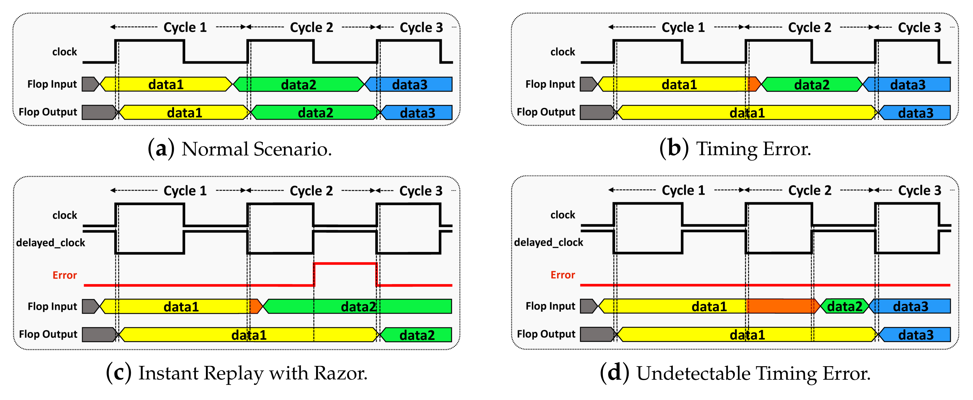
Figure 1. Multiple data-latching scenarios as the frequency of operation increases and the timing error detection window diminishes. In (a), baseline frequency is in operation. The frequency of operation is the same for (b,c) but higher than (a). The highest frequency of operation is employed in (d).
Jlpea 12 00032 g001
Figure 2. Rise of undetected timing errors with an increase in the operational frequency is shown in (a). The effects of the increasing timing errors are depicted in (b), where the classification accuracy drops drastically. This experimentation is performed on the Baseline TPU (Section 5.1).
Jlpea 12 00032 g002
Figure 3. Plots present the various timing error profiles during the high-frequency operations of the TPU.
Jlpea 12 00032 g003
Figure 4. Each MAC in the systolic array is enhanced with an MRFF. EMU comprises ECU and VCU. ECU collects and stores the timing error count from each cycle. VCU queries the timing error information from ECU to predict the operational clock cycles and boost the operating voltage during the predicted cycle interval.
Jlpea 12 00032 g004
Figure 5. (a) depicts the conversion of Razor Flip-Flop to Modified Razor Flip-Flop by altering the multiplexer input/output connections. The timing error correction capability of MRFF is shown in (b).
Jlpea 12 00032 g005
Figure 8. Cross-Layer Methodology.
Jlpea 12 00032 g008
Figure 9. Percentage of undetected timing errors mitigated by PREDITOR for eight different datasets.
Jlpea 12 00032 g009
Figure 10. Normalized Inference Accuracy (IA) of different comparative schemes and Voltage Boost Energy (BE) of Preditor for 8 DNN datasets at various normalized frequencies.
Jlpea 12 00032 g010
Figure 11. (a,b) depicts the power consumption and energy efficiency comparison of GoogleTPU with PREDITOR.
Jlpea 12 00032 g011
Table 1. List of DNN datasets.
Datasets
NameLayer Architecture
SVHN [17]CONV: (32, 32, 3) × (32, 32, 32) × (32, 32, 32) × (14, 14, 64) × (14, 14, 64) × (5, 5, 128) × (5, 5, 128),
FC: 512 × 512 × 10
GTSRB [18]CONV: (3, 48, 48) × (32, 48, 48) × (32, 46, 46) × (64, 23, 23)× (64, 21, 21) × (128, 10, 10) × (128, 8, 8),
FC: 2048 × 512 × 43
Reuters [19]FC: 2048 × 256 × 256 × 46
IMDB [20]CONV: 400 × (400x50) × (398, 256), FC: 256 × 1
MNIST [21]FC: 784 × 256 × 256 × 10
CIFAR-10 [22]CONV: (32, 32, 3) × (32, 32, 32) × (32, 32, 32) × (16, 16, 64) × (16, 16, 64) × (8, 8, 128) × (8, 8, 128),
FC: 2048 × 512 × 10
FMNIST [23]FC: 784 × 256 × 512 × 10
AMNIST [24]CONV: (20, 25, 1) × (20,25,128) × (20,25,64), FC: 32000 × 256 × 128 × 40
Publisher’s Note: MDPI stays neutral with regard to jurisdictional claims in published maps and institutional affiliations.