


Integrating ESG with Digital Twins and the Metaverse: A Data-Driven Framework for Smart Building Sustainability

 ,
, 
Abstract
1. Introduction
2. Research Question: Toward an Integrated Metaverse-Based Platform for Smart Building Management
3. Theoretical and Technological Framework
4. Development of the Environmental Dataset for Evaluating Smart Infrastructure Performance Through Digital Twin Integration
4.1. Environmental Key Performance Indicators (KPIs) for Digital Twin-Based Evaluation of Smart Infrastructure
4.2. Social and Environmental Key Performance Indicators (KPIs) for Digital Twin-Based Assessment of Smart Urban and Industrial Infrastructures
4.3. Governance Key Performance Indicators (KPIs) for ESG Evaluation in Digital Twin and Metaverse Applications
- Area (Area_m2—AREA): This signifies the total floor space investigated for the energy and environment indices related to the building or infrastructural facility. The total floor space is presented in square meters.
- Energy Consumption (Energy_Consumption_kWh—ENCO): This refers to the total consumption during the period under review, expressed in kilowatt-hours. This is the fundamental unit that can also produce comparative energy performance indicators
- Occupants (OCC): This variable measures the number of people using or occupying any given space. This parameter enables calculations related to energy use and per capita environmental factors, making analysis easier for the user.
5. Descriptive Statistical Analysis of the KPI Dataset for the Validation of a Digital Twin and Metaverse Prototype for Smart Buildings
6. Validation Framework and Data Reliability for ESG-Based Smart Building Model
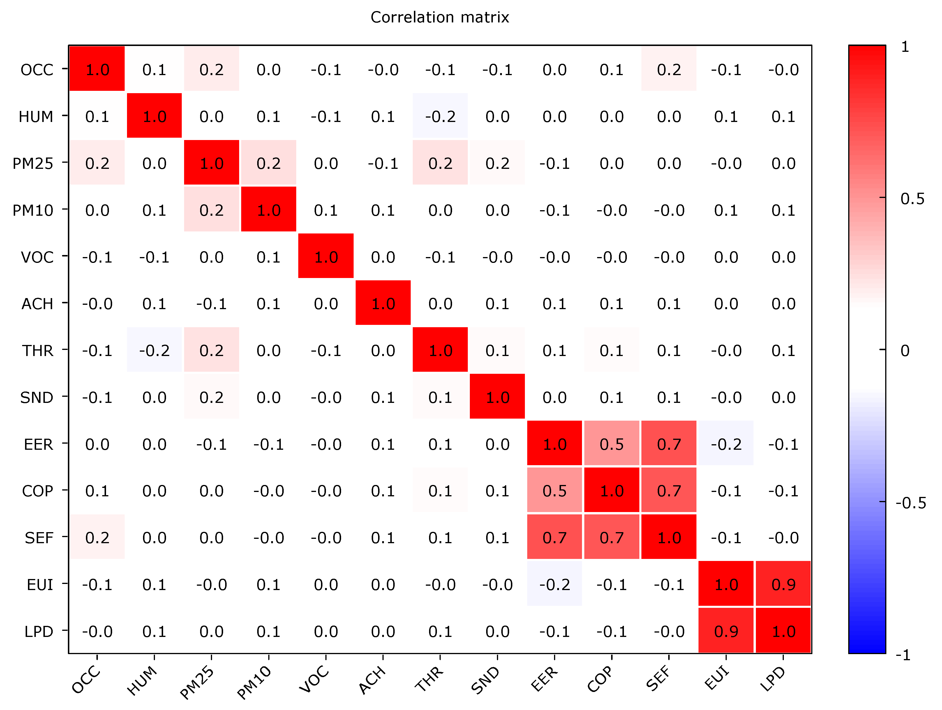
7. Scientific Validation of ESG Data Through Correlation Analysis for Smart Building Prototyping
7.1. Correlation Analysis and Validation of Environmental (E) Factors in the ESG Framework
7.2. Correlation Analysis and Validation of Social (S) Factors in the ESG Framework
7.3. Correlation Analysis and Validation of Governance (G) Factors in the ESG Framework
8. Regression-Based Validation of the ESG Dataset for Digital Twin Smart Building Modeling
9. Principal Component Analysis (PCA) for Technical Validation of the ESG Dataset in Smart Building Governance
9.1. Principal Component Analysis (PCA) Results for the Environmental (E) Dimension of the ESG Model
9.2. Principal Component Analysis (PCA) Results for the Social (S) Dimension of the ESG Model
9.3. Principal Component Analysis (PCA) Results for the Governance (G) Dimension of the ESG Model
10. Machine Learning Regression for ESG Dataset Validation in Digital Twin and Metaverse-Based Smart Building Governance
10.1. Random Forest Regression for Environmental Dataset Validation Within the ESG Framework
10.2. Machine Learning Validation of the Social (S) Component in the ESG Dataset
10.3. Machine Learning Validation of the Governance (G) Component Within the ESG Framework
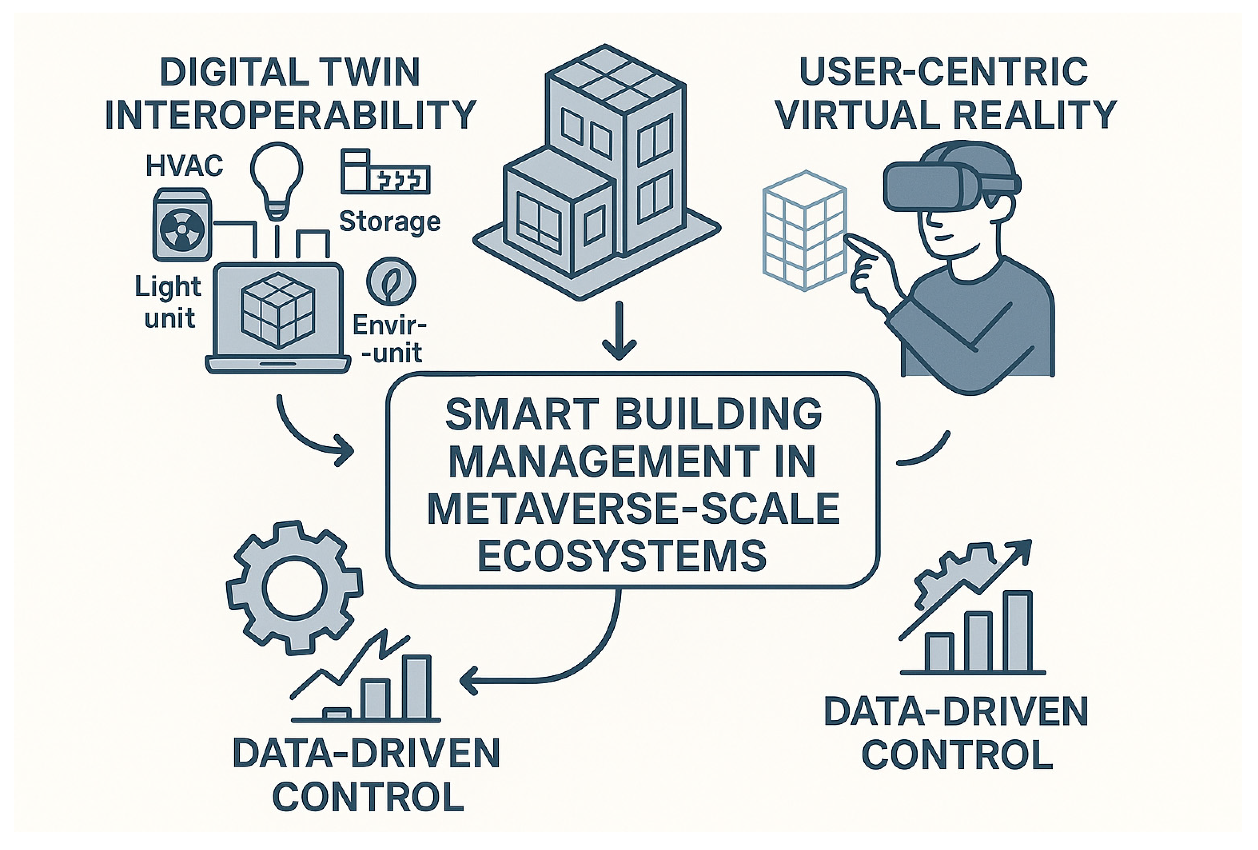
11. Theoretical Framework: Digital Twin Interoperability, User-Centered Virtual Environments, and Intelligent Data-Driven Control Systems in Smart Building Management
12. Operationalizing Environmental Sustainability Through Digital Twins: A Metaverse-Enhanced ESG Dashboard for Smart Building Management
12.1. Environmental Dimension Dashboard: Metaverse-Enhanced ESG Framework for Smart Building Digital Twin Development
12.2. Social Dimension Dashboard: Human-Centered ESG Framework for Digital Twin and Metaverse-Based Smart Building Management
12.3. Governance Dimension Dashboard: Financial Transparency and Strategic Decision-Making in Metaverse-Enhanced Smart Building Management
13. Discussion
14. Limitations
15. Conclusions
Author Contributions
Funding
Data Availability Statement
Conflicts of Interest
References
- Lemian, D.; Bode, F. Digital twins in the building sector: Implementation and key features. E3S Web Conf. 2025, 608, 05004. [Google Scholar] [CrossRef]
- Solmaz, A.Ş. Technological Advances in AEC: AI, Machine Learning, BIM, and the Future of Sustainable Building Design in a Post-Pandemic World. Black Sea J. Eng. Sci. 2024, 8, 757–774. [Google Scholar] [CrossRef]
- Fokaides, P.; Jurelionis, A.; Spudys, P. Boosting research for a smart and carbon neutral built environment with digital twins (SmartWins). In Proceedings of the 2022 IEEE International Smart Cities Conference (ISC2), Pafos, Cyprus, 26–29 September 2022; IEEE: New York City, NY, USA, 2022; pp. 1–4. [Google Scholar]
- Sabri, S.; Witte, P. Digital technologies in urban planning and urban management. J. Urban Manag. 2023, 12, 1–3. [Google Scholar] [CrossRef]
- Zavaleta, J.P.A. Digital Twins and BIM Toward the Smart Management of Post Occupancy Public Buildings. Preprints 2025. [Google Scholar] [CrossRef]
- Gao, Q.; Chu, Y.; Peng, Z.; Jin, Y.; Ji, X.; Ji, S.; Yue, Y. Smart Building Management System based on Digital Twin: A Case Study on Real-Time Environmental Monitoring and Thermal Comfort Prediction. In Proceedings of the 2024 IEEE International Symposium on Parallel and Distributed Processing with Applications (ISPA), Kaifeng, China, 30 October–2 November 2024. [Google Scholar]
- Matei, A.; Cocoșatu, M. Artificial Internet of Things, sensor-based digital twin urban computing vision algorithms, and blockchain cloud networks in sustainable smart city administration. Sustainability 2024, 16, 6749. [Google Scholar] [CrossRef]
- Misilmani, A.H.; Elbastawissi, I. Revolutionizing Urban Planning: Exploring the Synergy of BIM-GIS, Metaverse (VR & AR), and Real-World Applications to Urban Heritage Buildings in Beirut’s Rmeil and Medawar Clusters. MSA Eng. J. 2023, in press.
- Zhang, M.; Cao, J.; Sahni, Y.; Jiang, S.; Wu, T. EaaS: A service-oriented edge computing framework towards distributed intelligence. In Proceedings of the 16th IEEE International Conference on Service-Oriented System Engineering (SOSE), Newark, CA, USA, 15–18 August 2022; IEEE: New York City, NY, USA, 2022; pp. 165–175. [Google Scholar]
- Casini, M. Extended reality for smart building operation and maintenance: A review. Energies 2022, 15, 3785. [Google Scholar] [CrossRef]
- Din, I.U.; Awan, K.A.; Almogren, A.; Rodrigues, J.J.P.C. Integration of IoT and blockchain for decentralized management and ownership in the metaverse. Int. J. Commun. Syst. 2023, 36, e5612. [Google Scholar] [CrossRef]
- Masubuchi, Y.; Hiraki, T.; Hiroi, Y.; Ibara, M.; Matsutani, K.; Zaizen, M.; Morita, J. Development of Digital Twin Environment Through Integration of Commercial Metaverse Platform and IoT Sensors of Smart Building. In Proceedings of the 2025 IEEE Conference on Virtual Reality and 3D User Interfaces Abstracts and Workshops, Saint Malo, France, 8–12 March 2025; IEEE: New York City, NY, USA, 2025; pp. 852–855. [Google Scholar]
- Tang, M.; Nikolaenko, M.; Alrefai, A.; Kumar, A. Metaverse and digital twins in the age of AI and extended reality. Architecture 2025, 5, 36. [Google Scholar] [CrossRef]
- Elias, D.; Ziegenbein, D.; Mundhenk, P.; Hamann, A.; Rowe, A. The cyber-physical metaverse-where digital twins and humans come together. In Proceedings of the 2023 Design, Automation & Test in Europe Conference & Exhibition (DATE), Antwerp, Belgium, 17–19 April 2023; IEEE: New York City, NY, USA, 2023; pp. 1–2. [Google Scholar]
- Rafique, W.; Qadir, J. Internet of everything meets the metaverse: Bridging physical and virtual worlds with blockchain. Comput. Sci. Rev. 2024, 54, 100678. [Google Scholar] [CrossRef]
- Markopoulos, P.; Markopoulos, E.; Nandi, A.; Kantola, J. Integrating Digital Twins Into the Metaverse for Dynamic and Computer-Human Interactive Building Information Modelling. Sustain. Constr. Era Fourth Ind. Revolut. 2024, 149, 11–22. [Google Scholar]
- Stary, C. Digital process twins as intelligent design technology for engineering Metaverse/XR applications. Sustainability 2023, 15, 16062. [Google Scholar] [CrossRef]
- Picone, M.; Mariani, S.; Virdis, A.; Castagnetti, P. Digital Twin & Blockchain: Technology Enablers for Metaverse Computing. In Proceedings of the 2023 IEEE International Conference on Metaverse Computing, Networking and Applications (MetaCom), Kyoto, Japan, 26–28 June 2023; IEEE: New York City, NY, USA, 2023; pp. 1–8. [Google Scholar]
- Broo, D.G.; Bravo-Haro, M.; Schooling, J. Design and implementation of a smart infrastructure digital twin. Autom. Constr. 2022, 136, 104171. [Google Scholar] [CrossRef]
- Zahedi, F.; Alavi, H.; Sardroud, J.M.; Dang, H. Digital twins in the sustainable construction industry. Buildings 2024, 14, 3613. [Google Scholar] [CrossRef]
- Li, Y. AI-enhanced digital twins for energy efficiency and carbon footprint reduction in smart city infrastructure. Appl. Comput. Eng. 2025, 118, 42–47. [Google Scholar] [CrossRef]
- Alibrandi, U. Risk-informed digital twin of buildings and infrastructures for sustainable and resilient urban com-munities. ASCE-ASME J. Risk Uncertain. Eng. Syst. Part A Civ. Eng. 2022, 8, 04022032. [Google Scholar] [CrossRef]
- Chávez, C.A.G.; Bärring, M.; Frantzén, M.; Annepavar, A.; Gopalakrishnan, D.; Johansson, B. Achieving sustainable manufacturing by embedding sustainability kpis in digital twins. In Proceedings of the 2022 Winter Simulation Conference (WSC), Singapore, 11–14 December 2022; IEEE: New York City, NY, USA, 2022; pp. 1683–1694. [Google Scholar]
- Klar, R.; Angelakis, V. Linking Ports’ Digital Twins to Those of Cities. In Proceedings of the 2023 IEEE Smart World Congress (SWC), Portsmouth, UK, 28–31 August 2023; IEEE: New York City, NY, USA, 2023; pp. 1–8. [Google Scholar]
- Prandi, C.C.J.M.; Manzoni, P.; Peña-Haro, S.; Pierson, D.; Colom, W.; Senent, J. On integrating intelligent infrastructure and participatory monitoring for environmental modelling: The SMARTLAGOON approach. In Proceedings of the 2022 ACM Conference on Information Technology for Social Good, Limassol, Cyprus, 7–9 September 2022; pp. 236–243. [Google Scholar]
- Stipanovic, I.; Palic, S.S.; Casas, J.R.; Chacón, R.; Ganic, E. Inspection and maintenance KPIs to support decision making integrated into Digital Twin tool. Proc. Civ. Eng. 2023, 6, 1234–1241. [Google Scholar] [CrossRef]
- Yu, G.; Ye, X.; Xia, X.; Chen, Y. Digital twin enabled transition towards the smart electric vehicle charging in-frastructure: A review. Sustain. Cities Soc. 2024, 108, 105479. [Google Scholar] [CrossRef]
- Li, H.; Hong, T.; Lee, S.; Sofos, M. System-Level Key Performance Indicators for Building Performance Evaluation. Energy Build. 2020, 209, 109703. [Google Scholar] [CrossRef]
- Tennakoon, A.; Hewapathirana, D.; Jayathunga, R.; Dulani, H. A Guide for Carbon Footprint Assessment; The Climate Change Secretariat Ministry of Mahaweli Development and Environment: Battaramulla, Sri Lanka, 2016. [Google Scholar]
- Basu, P. Biomass Gasification, Pyrolysis and Torrefaction: Practical Design and Theory; Academic Press: Boston, MA, USA, 2018; ISBN 0-12-813040-7. [Google Scholar]
- Salom, J.; Marszal, A.; Widén, J.; Candanedo, J.; Lindberg, K. Analysis of Load Match and Grid Interaction Indicators in Net Zero Energy Buildings with Simulated and Monitored Data. Appl. Energy 2014, 136, 119–131. [Google Scholar] [CrossRef]
- Salom, J.; Widén, J.; Candanedo, J.; Sartori, I.; Voss, K.; Marszal, A. Understanding Net Zero Energy Buildings: Evaluation of Load Matching and Grid Interaction Indicators. In Proceedings of the Building Simulation, Sydney, Australia, 14–16 November 2011; Volume 6, pp. 2514–2521. [Google Scholar]
- Ala-Juusela, M.; Crosbie, T.; Hukkalainen, M. Defining and Operationalising the Concept of an Energy Positive Neighbourhood. Energy Convers. Manag. 2016, 125, 133–140. [Google Scholar] [CrossRef]
- Verbruggen, B.; Driesen, J. Grid Impact Indicators for Active Building Simulations. IEEE Trans. Sustain. Energy 2014, 6, 43–50. [Google Scholar] [CrossRef]
- Arteconi, A.; Polonara, F. Assessing the Demand Side Management Potential and the Energy Flexibility of Heat Pumps in Buildings. Energies 2018, 11, 1846. [Google Scholar] [CrossRef]
- Le Dréau, J.; Heiselberg, P. Energy Flexibility of Residential Buildings Using Short Term Heat Storage in the Thermal Mass. Energy 2016, 111, 991–1002. [Google Scholar] [CrossRef]
- Junker, R.; Azar, A.; Lopes, R.; Lindberg, K.; Reynders, G.; Relan, R.; Madsen, H. Characterizing the Energy Flexibility of Buildings and Districts. Appl. Energy 2018, 225, 175–182. [Google Scholar] [CrossRef]
- Kathirgamanathan, A.; Péan, T.; Zhang, K.; De Rosa, M.; Salom, J.; Kummert, M.; Finn, D. Towards Standardising Market-Independent Indicators for Quantifying Energy Flexibility in Buildings. Energy Build. 2020, 220, 110027. [Google Scholar] [CrossRef]
- Dovolil, P.; Svítek, M. Integrating ESG into the Smart City concept with focus on transport. In Proceedings of the 2024 Smart City Symposium Prague (SCSP), Prague, Czech Republic, 23–24 May 2024; IEEE: New York City, NY, USA, 2024; pp. 1–7. [Google Scholar]
- Barykin, S.E.; Strimovskaya, A.V.; Sergeev, S.M.; Borisoglebskaya, L.N.; Dedyukhina, N.; Sklyarov, I.; Saychenko, L. Smart city logistics on the basis of digital tools for ESG goals achievement. Sustainability 2023, 15, 5507. [Google Scholar] [CrossRef]
- Englezos, D.; Hadjidemetriou, L.; Papadopoulos, P.; Timotheou, S.; Polycarpou, M.; Panayiotou, C. A digital twin architecture for smart buildings. In Proceedings of the 2022 IEEE International Smart Cities Conference (ISC2), Paphos, Cyprus, 26–29 September 2022; IEEE: New York City, NY, USA, 2022; pp. 1–7. [Google Scholar]
- Hadjidemetriou, L.; Stylianidis, N.; Englezos, D.; Papadopoulos, P.; Eliades, D.; Timotheou, S.; Panayiotou, C. A digital twin architecture for real-time and offline high granularity analysis in smart buildings. Sustain. Cities Soc. 2023, 98, 104795. [Google Scholar] [CrossRef]
- Shaharuddin, S.; Abdul Maulud, K.N.; Syed Abdul Rahman, S.A.F.; Che Ani, A.I. Digital twin for indoor disaster in smart city: A systematic review. Int. Arch. Photogramm. Remote Sens. Spat. Inf. Sci. 2022, 46, 315–322. [Google Scholar] [CrossRef]
- Yitmen, I.; Almusaed, A.; Hussein, M.; Almssad, A. AI-Driven Digital Twins for Enhancing Indoor Environmental Quality and Energy Efficiency in Smart Building Systems. Buildings 2025, 15, 1030. [Google Scholar] [CrossRef]
- Lo, C.K. The Application of Digital Twin for Indoor Air Quality Management: A Case Study in Hong Kong. J. Sustain. Built Environ. 2025, 2, 11–22. [Google Scholar] [CrossRef]
- Saleh, S.; Abohamama, A.S.; Tolba, A.S. Intelligent Real-Time Air Quality Index Classification for Smart Home Digital Twins. Int. J. Adv. Comput. Sci. Appl. 2025, 16, 309–323. [Google Scholar] [CrossRef]
- Ariansyah, D.; Isnan, M.; Rahutomo, R.; Pardamean, B. Digital twin (DT) smart city for air quality management. Procedia Comput. Sci. 2023, 227, 524–533. [Google Scholar] [CrossRef]
- Venkateswarlu, N.; Sathiyamoorthy, M. Sustainable innovations in digital twin technology: A systematic review about energy efficiency and indoor environment quality in built environment. Front. Built Environ. 2025, 11, 1523464. [Google Scholar] [CrossRef]
- Peng, G.; Li, J.; Chen, Y.; Norizan, A.; Tay, L. High-Resolution Surface Relative Humidity Computation Using MODIS Image in Peninsular Malaysia. Chin. Geogr. Sci. 2006, 16, 260–264. [Google Scholar] [CrossRef]
- Kirešová, S.; Guzan, M. Measurement of Particulate Matter: Principles and Options of Measurement at Present. Acta Electrotech. Et Inform. 2022, 22, 8–18. [Google Scholar] [CrossRef]
- Vasudevan, J.; Coakley, D.; Angelopoulos, C.; Rastogi, P.; Sobek, O.; Jephson, G.; Eftekhari, M.; Dimitriou, V. Monitoring Indoor Environmental Quality (IEQ) in Buildings with Distributed Sensing; AIVC: Ghent, Belgium, 2023. [Google Scholar]
- Lu, X.; Lu, T.; Viljanen, M. Estimation of Space Air Change Rates and CO2 Generation Rates for Mechanically-Ventilated Buildings. In Advances in Computer Science and Engineering; IntechOpen: London, UK, 2011; pp. 237–260. [Google Scholar]
- Raouf, A.; Al-Ghamdi, S. Effect of R-Values Changes in the Baseline Codes: Embodied Energy and Environmental Life Cycle Impacts of Building Envelopes. Energy Rep. 2020, 6, 554–560. [Google Scholar] [CrossRef]
- Islam, S.; Bhat, G. Environmentally-Friendly Thermal and Acoustic Insulation Materials from Recycled Textiles. J. Environ. Manag. 2019, 251, 109536. [Google Scholar] [CrossRef]
- Andrade, Á.; Restrepo, A.; Tibaquirá, J. EER or Fcsp: A Performance Analysis of Fixed and Variable Air Conditioning at Different Cooling Thermal Conditions. Energy Rep. 2021, 7, 537–545. [Google Scholar] [CrossRef]
- Johra, H. Overview of the Coefficient of Performance (COP) for Conventional Vapour-Compression Heat Pumps in Buildings; Department of the Built Environment, Aalborg University: Aalborg, Denmark, 2022. [Google Scholar]
- Wu, W.; Fu, Y.; Wang, Z.; Liu, X.; Niu, Y.; Li, B.; Huang, G.Q. Consortium blockchain-enabled smart ESG reporting platform with token-based incentives for corporate crowdsensing. Comput. Ind. Eng. 2022, 172, 108456. [Google Scholar] [CrossRef]
- Zhang, S. Impact of Urban Digital Economy on ESG Performance: Do Technological and Business Model Innovation Matter. Innov. Econ. Front. 2025, 28, 14–30. [Google Scholar] [CrossRef]
- Hämäläinen, M. Smart city development with digital twin technology. In Proceedings of the 33rd Bled eConference-Enabling Technology for a Sustainable Society, Online, 28–29 June 2020. [Google Scholar]
- de Trizio, F.; Sciddurlo, G.; Cianci, I.; Piro, G.; Boggia, G. Optimizing key value indicators in intent-based networks through digital twins aided service orchestration mechanisms. Comput. Commun. 2024, 228, 107977. [Google Scholar] [CrossRef]
- Hu, L. Research on the application of Digital Twin in smart cities. Adv. Econ. Manag. Political Sci. 2023, 42, 14–20. [Google Scholar] [CrossRef]
- Ardebili, A.A.; Martella, C.; Longo, A.; Rucco, C.; Izzi, F.; Ficarella, A. IoT-Driven Resilience Monitoring: Case Study of a Cyber-Physical System. Appl. Sci. 2025, 15, 2092. [Google Scholar] [CrossRef]
- Hien, T.T.; Hanh, P.T.S. The direct effect of ESG reporting on firm performance: Empirical evidence from global firms during the early years of the green and digital twin transition. VNU Univ. Econ. Bus. 2024, 4, 1–12. [Google Scholar] [CrossRef]
- Becattini, M.; Fontani, G.; Paroli, L.; Iera, A. Digital Twin Networks for Sustainable In-network Computing in Future 6G Networks. In Proceedings of the 2024 IEEE 35th International Symposium on Personal, Indoor and Mobile Radio Communications (PIMRC), Valencia, Spain, 2–5 September 2024; IEEE: New York City, NY, USA, 2024; pp. 1–6. [Google Scholar]
- Zhang, M.; Yang, W.; Zhao, Z.; Pratap, S.; Wu, W.; Huang, G.Q. Is digital twin a better solution to improve ESG evaluation for vaccine logistics supply chain: An evolutionary game analysis. Oper. Manag. Res. 2023, 16, 1791–1813. [Google Scholar] [CrossRef]
- Suna, D.; Haas, R. How to Calculate Energy Savings and Costs of Energy Saving Obligations in a Harmonized Way. In Proceedings of the ECEEE Summer Study 2013, Toulon/Hyères, France, 3–8 June 2013. [Google Scholar]
- Hu, Y.; Chen, Y.; Tang, S.; Feng, L.; Huang, C. An Explanation of Energy Return on Investment From an Entropy Perspective. Front. Energy Res. 2021, 9, 633528. [Google Scholar] [CrossRef]
- Perpiñan, O.; Lorenzo, E.; Castro, M.; Eyras, R. Energy Payback Time of Grid Connected PV Systems: Comparison between Tracking and Fixed Systems. Prog. Photovolt. Res. Appl. 2009, 17, 137–147. [Google Scholar] [CrossRef]
- Thanos, G.; Minou, M.; Ganu, T.; Arya, V.; Chakraborty, D.; van Deventer, J.; Stamoulis, G. Evaluating Demand Response Programs by Means of Key Performance Indicators. In Proceedings of the 2013 Fifth International Conference on Communication Systems and Networks (COMSNETS), Bangalore, India, 7–10 January 2013; IEEE: New York City, NY, USA, 2013; pp. 1–6. [Google Scholar]
- Anna, R.; Simone, M.; Claudio, Z.; Giorgio, F. Key Performance Indicators of ‘Good Practices’ of Energy Efficiency in Industry: Application to Real Cases in Italy and in the European Union. Int. J. Energy Prod. Manag. 2017, 2, 239–250. [Google Scholar] [CrossRef][Green Version]
- Zhang, T.; Dornfeld, D. Energy Use per Worker-Hour: Evaluating the Contribution of Labor to Manufacturing Energy Use. In Proceedings of the Advances in Life Cycle Engineering for Sustainable Manufacturing Businesses: Proceedings of the 14th CIRP Conference on Life Cycle Engineering, Tokyo, Japan, 11–13 June 2007; pp. 189–193. [Google Scholar]
- Faria, P.; Lezama, F.; Vale, Z.; Khorram, M. A methodology for energy key performance indicators analysis. Energy Inform. 2021, 4, 6. [Google Scholar] [CrossRef]
- Alrashed, S. Key performance indicators for Smart Campus and Microgrid. Sustain. Cities Soc. 2020, 60, 102264. [Google Scholar] [CrossRef]
- Bandoria, L.H.; Cortes, B.; de Almeida, M.C. Statistical characterization of electricity use profile: Leveraging data analytics for stochastic simulation in a smart campus. Energy Build. 2024, 324, 114934. [Google Scholar] [CrossRef]
- Koutras, K.; Bompotas, A.; Halkiopoulos, C.; Kalogeras, A.; Alexakos, C. Dimensionality Reduction on IoT Monitoring Data of Smart Building for Energy Consumption Forecasting. In Proceedings of the 2023 IEEE International Smart Cities Conference (ISC2), Bucharest, Romania, 24–27 September 2023; IEEE: New York City, NY, USA, 2023; pp. 1–6. [Google Scholar]
- Ho, M.Y.; Lai, J.H.; Hou, H.; Zhang, D. Key performance indicators for evaluation of commercial building retrofits: Shortlisting via an industry survey. Energies 2021, 14, 7327. [Google Scholar] [CrossRef]
- Mustapha, Z.; Abilgah, T.; Tieru, C.K. Enhancing energy efficiency and management in smart buildings: A Holistic approach. J. Appl. Sci. Technol. Trends 2025, 6, 16–24. [Google Scholar] [CrossRef]
- Kumar, S.S.; Usha, P.; Balakrishnan, P.; Kannan, V.K.; Manjula, M.; Vijayakumar, M. Deep Learning Driven Engineering Innovations: Advancing Sustainable Green Building and Smart Infrastructure for a Resilient Future. In Proceedings of the 2024 First International Conference for Women in Computing (InCoWoCo), Pune, India, 14–15 November 2024; pp. 1–5. [Google Scholar]
- Romanska-Zapala, A.; Dudek, P.; Górny, M.; Dudzik, M. Modular statistical system for an integrated environmental control. E3S Web Conf. 2020, 172, 19006. [Google Scholar] [CrossRef]
- Hakawati, B.; Mousa, A.; Draidi, F. Smart energy management in residential buildings: The impact of knowledge and behavior. Sci. Rep. 2024, 14, 1702. [Google Scholar] [CrossRef]
- Arias-Requejo, D.; Pulido, B.; Keane, M.M.; Alonso-González, C.J. Clustering and deep-learning for energy consumption forecast in smart buildings. IEEE Access 2023, 11, 128061–128080. [Google Scholar] [CrossRef]
- Wang, Q. Correlation Analysis of ESG Ratings and Enterprise Performance. Asia Pac. Econ. Manag. Rev. 2024, 1, 57–63. [Google Scholar] [CrossRef]
- Eskantar, M.; Zopounidis, C.; Doumpos, M.; Galariotis, E.; Guesmi, K. Navigating ESG complexity: An in-depth analysis of sustainability criteria, frameworks, and impact assessment. Int. Rev. Financ. Anal. 2024, 95, 103380. [Google Scholar] [CrossRef]
- Handoko, S.; Afifudin, A.; Holili, M.H. The Strategic Integration of ESG Metrics in Performance Evaluation: Insights from Management Accounting Practices. J. Manag. Inform. 2024, 3, 141–156. [Google Scholar] [CrossRef]
- Hou, Z.; Li, D.; Jin, F.; Zhang, Y.; Luo, W. Green supply chain knowledge networks and corporate ESG performance: The role of green technology innovation and knowledge integration capability. Int. J. Prod. Res. 2025, 63, 4306–4327. [Google Scholar] [CrossRef]
- Zhou, L. Trustworthy digital twinning data platform for power infrastructure construction projects using blockchain and semantic web. Front. Built Environ. 2024, 10, 1440513. [Google Scholar] [CrossRef]
- Du, Q.; Sun, Z.; Goodell, J.W.; Du, A.M.; Yang, T. Ecological risk and corporate sustainability: Examining ESG performance, risk management, and productivity. Int. Rev. Financ. Anal. 2024, 96, 103551. [Google Scholar] [CrossRef]
- Wang, Y. A Study Of LYFEN’S ESG Disclosure and Its Impact on Corporate Performance. In Highlights in Business, Economics and Management; Darcy & Roy Press Co., Ltd.: Hillsboro, OR, USA, 2024; Volume 40, pp. 391–397. [Google Scholar]
- Ioannidis, E.; Tsoumaris, D.; Ntemkas, D.; Sarikeisoglou, I. Correlations of ESG ratings: A signed weighted network analysis. AppliedMath 2022, 2, 638–658. [Google Scholar] [CrossRef]
- Loukılı, M.; Benlı, V.F. Elaborating ESG criteria in investments. Press. Procedia 2023, 17, 228–229. [Google Scholar]
- Sorathiya, A.; Saval, P.; Sorathiya, M. Data-driven sustainable investment strategies: Integrating ESG, financial data science, and time series analysis for alpha generation. Int. J. Financ. Stud. 2024, 12, 36. [Google Scholar] [CrossRef]
- Cai, J.; Chen, J.; Hu, Y.; Li, S.; He, Q. Digital twin for healthy indoor environment: A vision for the post-pandemic era. Front. Eng. Manag. 2023, 10, 300–318. [Google Scholar] [CrossRef]
- Ni, Z.; Zhang, C.; Karlsson, M.; Gong, S. Edge-based Parametric Digital Twins for Intelligent Building Indoor Climate Modeling. In Proceedings of the 2024 IEEE 20th International Conference on Factory Communication Systems (WFCS), Toulouse, France, 17–19 April 2024; IEEE: New York City, NY, USA, 2024; pp. 1–8. [Google Scholar]
- Islam, M.B.; Guerrieri, A.; Gravina, R.; Fortino, G. A Deep Learning Based Digital Twin for Indoor Temperature Prediction in Smart Buildings. In Proceedings of the 2024 IEEE Conference on Pervasive and Intelligent Computing (PICom), Boracay Island, Philippines, 5–8 November 2024; IEEE: New York City, NY, USA, 2024; pp. 83–89. [Google Scholar]
- Hii, D.J.C.; Hasama, T. Towards the Digital Twinning and Simulation of a Smart Building for Well-Being. In Proceedings of the 2024 Winter Simulation Conference (WSC), Orlando, FL, USA, 15–18 December 2024; IEEE: New York City, NY, USA, 2024; pp. 726–737. [Google Scholar]
- Ravid, B.Y.; Aharon-Gutman, M. The social digital twin: The social turn in the field of smart cities. Environ. Plan. B Urban Anal. City Sci. 2023, 50, 1455–1470. [Google Scholar] [CrossRef]
- Roda-Sanchez, L.; Cirillo, F.; Solmaz, G.; Jacobs, T.; Garrido-Hidalgo, K.E. Building a smart campus digital twin: System, analytics, and lessons learned from a real-world project. IEEE Internet Things J. 2023, 11, 4614–4627. [Google Scholar] [CrossRef]
- Poels, G.; Proper, H.A.; Bork, D. DT4GITM: Vision for a framework for digital twin enabled IT governance. In Proceedings of the 55th Hawaii International Conference on System Sciences, Maui, HI, USA, 4–7 January 2022; pp. 6626–6635. [Google Scholar]
- Kljaić, Z.; Grdić, M.; Mlinarić, T.J.; Nikšić, M.; Pavković, D.; Cipek, M. Digital Twin Models with ESG Methodology as a Tool for the Transformation of Cities in the Area of Transport and Energy. In Proceedings of the 2024 47th MIPRO ICT and Electronics Convention (MIPRO), Opatija, Croatia, 20–24 May 2024; IEEE: New York City, NY, USA, 2024; pp. 1937–1942. [Google Scholar]
- Elnour, M.; Ahmad, A.M.; Abdelkarim, S.; Fadli, F.; Naji, K. Empowering smart cities with digital twins of buildings: Applications and implementation considerations of data-driven energy modelling in building management. Sustain. Cities Soc. 2024, 69, 102816. [Google Scholar] [CrossRef]
- Chungath, J.; Hacks, S. Requirements for a Digital Twin for Energy, Social, and Governance Data of Commercial Buildings. In Proceedings of the International Conference on Business Process Modeling, Development and Support, Limassol, Cyprus, 3–4 June 2024; Springer Nature: Cham, Switzerland, 2024; pp. 341–351. [Google Scholar]
- Cureton, P.; Dunn, N. Digital twins of cities and evasive futures. In Shaping Smart for Better Cities; Academic Press: Boston, MA, USA, 2021; pp. 267–282. [Google Scholar]
- Pileggi, P.; Lazovik, E.; Broekhuijsen, J.; Borth, M.; Verriet, J. Lifecycle governance for effective digital twins: A joint systems engineering and IT perspective. In Proceedings of the 2020 IEEE International Systems Conference (SysCon), Montreal, QC, Canada, 24 August–20 September 2020; IEEE: New York City, NY, USA, 2020; pp. 1–8. [Google Scholar]
- Lv, Z.; Cheng, C.; Lv, H. Digital twins for secure thermal energy storage in building. Appl. Energy 2023, 338, 120907. [Google Scholar] [CrossRef]
- Yue, A.; Mao, C.; Zhao, S. Smart governance of urban ecological environment driven by digital twin technology: A case study on the ecological restoration and management in s island of chongqing. IOP Conf. Ser. Earth Environ. Sci. 2022, 1101, 072003. [Google Scholar] [CrossRef]
- Hartmann, M.; Pawelzik, S.; Wimmer, M.A. Comparative Analysis of Digital Twins in Smart Cities. In Proceedings of the EGOV-CeDEM-ePart Conference, Ghent University and KU Leuven, Ghent/Leuven, Belgium, 1–5 September 2023. [Google Scholar]
- Cranford, R. Conceptual application of digital twins to meet ESG targets in the mining industry. Front. Ind. Eng. 2023, 1, 1223989. [Google Scholar] [CrossRef]
- Dou, X.; Yin, S. The impact of ESG on corporate financial performance: Based on fixed effects regression model. J. Comput. Methods Sci. Eng. 2024, 24, 2719–2731. [Google Scholar] [CrossRef]
- Liu, X.; Liao, K.T.; Wang, J.; Wu, S.; Su, Y. Topic mining and evolution analysis of digital governance in Chinese enterprises based on the BERTopic model. Chin. Manag. Stud. 2025. [Google Scholar] [CrossRef]
- Guo, Y.; Chen, C.; Luo, X.; Martek, I. Critical drivers and barriers of digital twin adoption in water infrastructure: An environmental, social, governance, and financial perspective. Sustain. Dev. 2025, 33, 1623–1648. [Google Scholar] [CrossRef]
- Su, J.; Sun, Y. An improved TOPSIS model based on cumulative prospect theory: Application to ESG performance evaluation of state-owned mining enterprises. Sustainability 2023, 15, 10046. [Google Scholar] [CrossRef]
- Chen, D.; Lin, H. Study on the impact of ESG performance on financial performance of firms based on multiple linear regression models. In Proceedings of the 2023 IEEE 3rd International Conference on Social Sciences and Intelligence Management (SSIM), Taichung, Taiwan, 15–17 December 2023; pp. 320–323. [Google Scholar]
- Berman, S.L.; Wicks, A.C.; Kotha, S.; Jones, T.M. Does stakeholder orientation matter? The relationship between stakeholder management models and firm financial performance. Acad. Manag. J. 1999, 42, 488–506. [Google Scholar] [CrossRef]
- Lai, K.E.; Rahiman, N.A.; Othman, N.; Ali, K.N.; Lim, Y.W.; Moayedi, F.; Dzahir, M.A.M. Quantification process of carbon emissions in the construction industry. Energy Build. 2023, 289, 113025. [Google Scholar] [CrossRef]
- Ascione, F.; De Masi, R.F.; Mastellone, M.; Vanoli, G. Building rating systems: A novel review about capabilities, current limits and open issues. Sustain. Cities Soc. 2022, 76, 103498. [Google Scholar] [CrossRef]
- Zhou, H.; Ji, S.; Zhang, Q.; Jin, W.; Feng, A.; Lin, C.; Li, Q. Wastewater treatment: A universal, scalable and recyclable catalyst with adjustable activity for diverse dyes degradation. J. Environ. Manag. 2023, 330, 117188. [Google Scholar] [CrossRef]
- Bonab, A.B.; Bellini, F.; Rudko, I. Theoretical and analytical assessment of smart green cities. J. Clean. Prod. 2023, 410, 137315. [Google Scholar] [CrossRef]
- Ma, S.; Huang, Y.; Liu, Y.; Kong, X.; Yin, L.; Chen, G. Edge-cloud cooperation-driven smart and sustainable production for energy-intensive manufacturing industries. Appl. Energy 2023, 337, 120843. [Google Scholar] [CrossRef]
- Hu, L.; Lu, S. Comparison of Thermal Comfort Models Based on Principal Component Analysis and Ant Colony Optimization. In Proceedings of the 2024 2nd International Conference on Artificial Intelligence and Automation Control (AIAC), Guangzhou, China, 20–22 December 2024; IEEE: New York City, NY, USA, 2024; pp. 67–70. [Google Scholar]
- Bezrukov, A.; Sadovnikova, N.; Lebedinskaya, O. Incorporating the Current Tendencies and Condition of the Financial Market of Russian Federation into Regional Cluster Modelling upon Principal Factor Analysis of Government Bonds. SSRN 2022, 4265198. [Google Scholar] [CrossRef]
- Pandhare, V.; Negri, E.; Ragazzini, L.; Cattaneo, L.; Macchi, M.; Lee, J. Digital twin-enabled robust production scheduling for equipment in degraded state. J. Manuf. Syst. 2024, 74, 841–857. [Google Scholar] [CrossRef]
- Zhang, Z.; Yu, J.; Tian, J. Community participation, social capital cultivation and sustainable community renewal: A case study from Xi’an’s southern suburbs, China. J. Knowl. Econ. 2024, 15, 11007–11040. [Google Scholar] [CrossRef]
- Inala, K.P.; Teja, K.K.; Reddy, K.S.; Archana, K. Optimal Load Prediction in a Smart Metering Network Using Random Forest Algorithm. In Proceedings of the 2024 Third International Conference on Power, Control and Computing Technologies (ICPC2T), Raipur, India, 18–20 January 2024. [Google Scholar]
- Ji, C.; Niu, Y. A hybrid evolutionary and machine learning approach for smart city planning: Digital twin approach. Sustain. Energy Technol. Assess. 2024, 64, 103650. [Google Scholar] [CrossRef]
- Ukwuoma, H.C.; Dusserre, G.; Coatrieux, G.; Vincent, J.; Ahmed, N.B. Optimising Intrusion Detection in Cyber-Physical Systems. In Proceedings of the 2024 8th Cyber Security in Networking Conference (CSNet), Paris, France, 4–6 December 2024; IEEE: New York, NY, USA, 2024; pp. 7–14. [Google Scholar]
- Vasilica, B.V.; Anton, F.D.; Pietraru, R.; Anton, S.O.; Chiriac, B.N. Enhancing Security in Smart Robot Digital Twins Through Intrusion Detection Systems. Appl. Sci. 2025, 15, 4596. [Google Scholar] [CrossRef]
- Du, Z. Prediction of Building Energy Consumption Based on LSTM-SVR-Random Forest Hybrid Model. Appl. Comput. Eng. 2024, 115, 75–85. [Google Scholar] [CrossRef]
- Kinshakov, E.; Parfenenko, Y.; Shendryk, V. Comparative analysis of methods for prediction continuous numerical features on big datasets. Technol. Audit. Prod. Reserves 2021, 6, 15–17. [Google Scholar] [CrossRef]
- Miao, Y.; Xu, Y. Random Forest-Based Analysis of Variability in Feature Impacts. In Proceedings of the 2024 IEEE 2nd International Conference on Image Processing and Computer Applications (ICIPCA), Shenyang, China, 28–30 June 2024; IEEE: New York City, NY, USA, 2024; pp. 1130–1135. [Google Scholar]
- Orlenko, A.; Moore, J.H. Improving the interpretability of random forest models of genetic association in the presence of non-additive interactions. Res. Sq. 2020. [Google Scholar] [CrossRef]
- Yu, F.; Wei, C.; Deng, P.; Peng, T.; Hu, X. Deep exploration of random forest model boosts the interpretability of machine learning studies of complicated immune responses and lung burden of nanoparticles. Sci. Adv. 2021, 7, eabf4130. [Google Scholar] [CrossRef]
- Li, W.; Xu, X. A hybrid evolutionary and machine learning approach for smart building: Sustainable building energy management design. Sustain. Energy Technol. Assess. 2024, 65, 103709. [Google Scholar] [CrossRef]
- Gaur, L.; Singh, G.; Solanki, A.; Jhanjhi, N.Z.; Bhatia, U.; Sharma, S.; Kim, W. Disposition of youth in predict-ing sustainable development goals using the neuro-fuzzy and random forest algorithms. Hum.-Centric Comput. Inf. Sci. 2021, 12, 11. [Google Scholar]
- Li, G.; Jiang, L. Random Forest Algorithm-based Modelling and Neural Network Analysis Between Social Anxiety Disorder of Childhood and Parents’ Socioeconomic Attributes. In Proceedings of the 2023 IEEE 6th Eurasian Conference on Educational Innovation (ECEI), Singapore, 3–5 February 2023; pp. 222–225. [Google Scholar]
- Khan, Z.; Vora, N. Predicting Consumer Shifts to Sustainable Products using Machine Learning Models. J. Inf. Technol. Digit. World 2024, 6, 302–316. [Google Scholar] [CrossRef]
- Xu, Y. Design of human resource allocation algorithm based on improved random forest. In Proceedings of the 2021 International Conference on Aviation Safety and Information Technology, Changsha, China, 18–20 December 2021; pp. 656–661. [Google Scholar]
- Chowdhury, M.A.F.; Abdullah, M.; Azad, M.A.K.; Sulong, Z.; Islam, M.N. Environmental, social and governance (ESG) rating prediction using machine learning approaches. Ann. Oper. Res. 2023, 1–25. [Google Scholar] [CrossRef]
- Lou, X. Evaluation of College Students’ Innovation and Entrepreneurship Abilities in the New Media Environment Using Tree Soft Set and Neutrosophic Modeling. Neutrosophic Sets Syst. 2025, 85, 22. [Google Scholar]
- Ozdemir, G.; Kuzlu, M.; Catak, F.O. Machine learning insights into forecasting solar power generation with explainable AI. Electr. Eng. 2025, 107, 7329–7350. [Google Scholar] [CrossRef]
- Drobnič, F.; Kos, A.; Pustišek, M. On the interpretability of machine learning models and experimental feature selection in case of multicollinear data. Electronics 2020, 9, 761. [Google Scholar] [CrossRef]
- Akhtar, K.; Yaseen, M.U.; Imran, M.; Khattak, S.B.A.; Nasralla, M.M. Predicting inmate suicidal behavior with an interpretable ensemble machine learning approach in smart prisons. PeerJ Comput. Sci. 2024, 10, e2051. [Google Scholar] [CrossRef]
- Wang, X. Construction and optimization of enterprise ESG performance evaluation model based on support vector machine. In Proceedings of the Second International Conference on Big Data, Computational Intelligence, and Applications (BDCIA 2024), Huanggang, China, 15–17 November 2024; SPIE: Bellingham, WA, USA, 2025; Volume 13550, pp. 748–754. [Google Scholar]
- Wu, Z.; Yang, L.; Fei, Y.; Wang, X. Regularization methods for sparse ESG-valued multi-period portfolio optimization with return prediction using machine learning. Expert Syst. Appl. 2023, 232, 120850. [Google Scholar] [CrossRef]
- Lin, H.Y.; Hsu, B.W. Empirical study of ESG score prediction through machine learning—A case of non-financial companies in Taiwan. Sustainability 2023, 15, 14106. [Google Scholar] [CrossRef]
- Koseoglu, M.A.; Arici, H.E.; Saydam, M.B.; Olorunsola, V.O. Predictive roles of environment, social, and governance scores on firms’ diversity: A machine learning approach. Nankai Bus. Rev. Int. 2025, 16, 284–306. [Google Scholar] [CrossRef]
- Suprihadi, E.; Danila, N. Forecasting ESG stock indices using a machine learning approach. Glob. Bus. Rev. 2024, 09721509241234033. [Google Scholar] [CrossRef]
- Aloqaily, M.; Bouachir, O.; Karray, F.; Al Ridhawi, I.; El Saddik, A. Integrating digital twin and advanced intelligent technologies to realize the metaverse. IEEE Consum. Electron. Mag. 2022, 12, 47–55. [Google Scholar] [CrossRef]
- Lyu, Z.; Fridenfalk, M. Digital twins for building industrial metaverse. J. Adv. Res. 2024, 66, 31–38. [Google Scholar] [CrossRef]
- Li, X.; Yang, Y.; Xie, B.; He, Z.; Chen, J.; Gan, W. AI-Driven Metaverse Digital Twin Cities: Prototype Platform Design for Integrated Virtual Urban Ecosystems and Services. In Proceedings of the 2024 3rd International Conference on Automation, Robotics and Computer Engineering (ICARCE), Virtual, 17–18 December 2024; IEEE: New York City, NY, USA, 2024; pp. 393–399. [Google Scholar]
- Ruiu, P.; Nitti, M.; Pilloni, V.; Cadoni, M.; Grosso, E.; Fadda, M. Metaverse & human digital twin: Digital identity, biometrics, and privacy in the future virtual worlds. Multimodal Technol. Interact. 2024, 8, 48. [Google Scholar] [CrossRef]
- Zainab; Bawanay, N.Z. Digital Twin, Metaverse and Smart Cities in a Race to the Future. In Proceedings of the 2023 24th International Arab Conference on Information Technology (ACIT), Ajman, United Arab Emirates, 6–8 December 2023; IEEE: New York, NY, USA, 2023; pp. 1–8. [Google Scholar]
- Stefko, R.; Michalikova, K.F.; Strakova, J.; Novak, A. Digital twin-based virtual factory and cyber-physical production systems, collaborative autonomous robotic and networked manufacturing technologies, and enterprise and business intelligence algorithms for industrial metaverse. Equilibrium 2025, 20, 389–425. [Google Scholar] [CrossRef]
- Farsangi, E.N.; Shehata, A.O.; Rashidi, M.; Ghassempour, N.; Mirjalili, S. Transitioning from BIM to digital twin to metaverse. Front. Built Environ. 2024, 10, 1486423. [Google Scholar] [CrossRef]
- Mahariya, S.K.K.A.; Singh, R.; Gehlot, A.; Akram, S.V.; Twala, B.; Priyadarshi, N. Smart campus 4.0: Digitalization of university campus with assimilation of industry 4.0 for innovation and sustainability. J. Adv. Res. Appl. Sci. Eng. Technol. 2023, 32, 120–138. [Google Scholar] [CrossRef]
- Hassani, H.; Huang, X.; MacFeely, S. Enabling digital twins to support the UN SDGs. Big Data Cogn. Comput. 2022, 6, 115. [Google Scholar] [CrossRef]
- Hernandez, M.S.; Sentosa, I.; Gaudreault, F.; Davison, I.; Sharin, F.H. The emergence of the metaverse in the digital blockchain economy: Applying the ESG framework for a sustainable future. In Proceedings of the 2023 3rd International Conference on Advance Computing and Innovative Technologies in Engineering (ICACITE), Greater Noida, India, 12–13 May 2023; IEEE: New York, NY, USA, 2023; pp. 1324–1329. [Google Scholar]
- Adnan, M.; Ahmed, I.; Iqbal, S.; Fazal, M.R.; Siddiqi, S.J.; Tariq, M. Exploring the convergence of Metaverse, Blockchain, Artificial Intelligence, and digital twin for pioneering the digitization in the envision smart grid 3.0. Comput. Electr. Eng. 2024, 120, 109709. [Google Scholar] [CrossRef]
- Park, J.; Choi, W.; Jeong, T.; Seo, J. Digital twins and land management in South Korea. Land Use Policy 2023, 124, 106442. [Google Scholar] [CrossRef]
- Trung, D.Q. Keynote talk# 2: From digital twin to metaverse: The role of 6G edge intelligence-based ultra-reliable and low latency communications. In Proceedings of the 2022 RIVF International Conference on Computing and Communication Technologies (RIVF), Ho Chi Minh City, Vietnam, 20–22 December 2022. [Google Scholar]
- Duong, T.Q.; Van Huynh, D.; Khosravirad, S.R.; Sharma, V.; Dobre, O.A.; Shin, H. From digital twin to metaverse: The role of 6G ultra-reliable and low-latency communications with multi-tier computing. IEEE Wirel. Commun. 2023, 30, 140–146. [Google Scholar] [CrossRef]
- Kuru, K. Metaomnicity: Toward immersive urban metaverse cyberspaces using smart city digital twins. IEEE Access 2023, 11, 43844–43868. [Google Scholar] [CrossRef]
- Chambon, A.; Sahli, A.; Rachedi, A.; Mebarki, A. Optimizing iot networks deployment under connectivity constraint for dynamic digital twin. In Proceedings of the 2023 IEEE International Conference on Metaverse Computing, Networking and Applications (MetaCom), Kyoto, Japan, 26–28 June 2023; IEEE: New York City, NY, USA, 2023; pp. 474–480. [Google Scholar]
- Jagatheesaperumal, S.K.; Yang, Z.; Yang, Q.; Huang, C.; Xu, W.; Shikh-Bahaei, M.; Zhang, Z. Semantic-aware digital twin for metaverse: A comprehensive review. IEEE Wirel. Commun. 2023, 30, 38–46. [Google Scholar] [CrossRef]







| Ref. | Type | Methodology | Inclusion Criterion | Main Conclusion | Relevance for Our Study |
|---|---|---|---|---|---|
| [9] | Technical study | Simulation-based system architecture analysis for intelligent building networks | Addresses integration of intelligent computing systems for smart building networks | Demonstrates that distributed control enhances communication and data flow efficiency | Provides the foundation for connecting digital twin data with real-time management systems |
| [10] | Review paper | Systematic review of XR applications in building operation and maintenance | Focuses on extended reality (XR) for maintenance and user experience in smart buildings | Shows that XR improves monitoring, maintenance, and user engagement | Informs the immersive visualization layer of the proposed metaverse-based management framework |
| [11] | Conceptual framework | Analytical study integrating IoT and blockchain technologies for decentralized data management | Examines blockchain–IoT convergence for transparent smart building data handling | Highlights traceability and security benefits of decentralized systems | Supports the governance and transparency dimension in ESG-related metrics |
| [12] | Experimental study | Empirical testing using IoT sensors and commercial metaverse platforms | Investigates how physical IoT data interact with virtual metaverse spaces | Validates feasibility of real-time immersive visualization | Demonstrates the interoperability between physical and virtual building environments |
| [13] | Theoretical model | Conceptual modelling and synthesis of digital twin–metaverse integration | Explores merging digital twin and metaverse paradigms for smart building management | Proposes a conceptual framework for immersive, data-driven control of buildings | Provides the theoretical baseline for designing the integrated digital management model proposed in this research |
| KPI | Acronym | Description | Formula |
|---|---|---|---|
| Carbon Footprint | CFPT | Indicates the total amount of greenhouse gas (GHG) emissions caused by an individual, organization, or product, either directly or indirectly. The formula calculates the sum of emissions associated with different activities by multiplying the quantity of each activity by its corresponding emission factor [30]. | |
| = Quantity of a specific activity that generates greenhouse gas emissions (e.g., km, kWh, liters). = Rate of GHG emissions per unit of activity, expressed in CO2 equivalent per unit (e.g., tCO2e/kWh for electricity, tCO2e/liter for fuel, etc.). | |||
| Emission Intensity EI | EMIN | Evaluates the environmental impact of an energy system by measuring the amount of carbon dioxide (CO2) emitted per unit of energy consumed or produced. A low value indicates that the system is more environmentally efficient, emitting less CO2 for each unit of energy consumed or produced (this can occur through the use of renewable energy sources). Conversely, high values typically occur in systems that rely heavily on fossil fuels [31]. | EI |
| = Total amount of CO2 emitted over a given period, resulting from the consumption of fossil fuels or the use of grid electricity [tCO2] = Total amount of energy consumed or produced during the same reference period [kWh] | |||
| Load Cover Factor | LCF | Represents the ratio between the energy actually supplied by a generation source and the energy demanded or consumed over a given time interval. If equal to 1, it indicates that the generation capacity exceeds the demand, whereas values lower than 1 indicate that generation is insufficient to meet the required load. When = 1, the entire load demand is fully satisfied. When 1, the load is not completely met during part of the period, due to limitations in generation or available resources. Range: 0 1 [32,33]. | |
| = On-site energy generation at a given time t [kWh] = Storage energy losses at a given time t [kWh] = Building load at a given time t [kWh] e = Start and end of the evaluation period [s] = Storage energy balance at a given time t [kWh] | |||
| = Charging energy of the storage system [kWh] = Discharging energy of the storage system [kWh] | |||
| Supply Cover Factor | SCF | Indicates the ability of an organization to meet its energy demand through its own on-site supply resources. When = 1, the amount of useful supplied resources is exactly equal to the total available amount. This implies that there are no significant losses and that all available resources are fully utilized. When < 1, the amount of effectively usable resources is lower than the total available amount. Part of the generated energy is not used to meet the load, likely due to overproduction, losses, or storage capacity limitations. Range: 0 1 [32,33]. | |
| = On-site energy generation at a given time t [kWh] = Storage energy losses at a given time t [kWh] = Building load at a given time t [kWh] e = Start and end of the evaluation period [s] = Storage energy balance at a given time t [kWh] | |||
| = Charging energy of the storage system [kWh] = Discharging energy of the storage system [kWh] | |||
| Load Matching Index | LMI | Measures the efficiency with which on-site energy generation (whether renewable or not) matches the energy load (demand) of a system. It evaluates how well the energy production profile corresponds to the load profile over time by analyzing the synchrony between supply and demand. A higher index indicates a better match between generation and load. When = 1, the load is fully met (i.e., generation and storage are sufficient to cover the required demand) in every considered interval. When < 1, the load is not fully met at certain times, meaning that the generation and/or storage capacity was lower than the demand. Range: 0% ≤ f_(load,i) ≤ 100% [33]. | |
| i = Time intervals [hourly, daily, monthly] = On-site energy generation at a given time t [kWh] = Storage energy balance at a given time t [kWh] = Energy losses at a given time t (sum of generation energy losses, storage energy losses, building technical system losses (excluding storage), and load-related energy losses such as distribution losses) [kWh] = Building load at a given time t [kWh] e = Start and end of the evaluation period [s] = Number of samples within the evaluation period, from τ1 to τ2. When hourly data are used and the evaluation period covers a full year, the number of samples is 8760. | |||
| On-site Energy Ratio | OER | Determines the amount of energy produced on-site (e.g., from renewable sources such as solar panels or wind turbines) relative to the total energy consumption over a given period of time. If = 1, the on-site generated energy equals the total energy consumption. If < 1, the on-site produced energy is lower than total consumption, meaning that the system depends on external energy sources to meet the demand. If > 1, the on-site generated energy exceeds total consumption, indicating that energy production is greater than demand (and surplus energy may be exported to the grid). Range: 0 [34]. | |
| = On-site energy generation at a given time t [kWh] = Total energy consumption (energy load) at a given time t [kWh] e = Start and end of the evaluation period [s] | |||
| Grid Interaction Index (Indice di Interazione con la Rete) | GII | Measures the level of interaction and integration of a facility with the power grid, describing its average stress. If = 100%, the energy exchanged with the grid during interval i equals the maximum possible exchange. If = 0%, no energy exchange with the grid occurred at that moment. If < 0%, energy was injected into the grid rather than drawn from it [32,33]. | |
| = Net energy exchanged with the power grid during interval i (can be positive or negative depending on whether energy is being drawn from or injected into the grid) [kWh] = Maximum absolute value of the net energy flow with the grid, taken over all considered time intervals [kWh] i = Time intervals [hourly, daily, monthly] | |||
| No grid interaction probability | NGI | Measures the probability that a building or facility operates autonomously from the power grid, and therefore the likelihood of no interaction with it. It also indicates the extent to which the load is covered by stored energy or renewable energy use. If = 0, there was no moment during the considered time interval when the net energy was zero or negative. If = 1, the net energy was zero or negative for the entire considered period. Range: 0 1 [32,33]. | |
| = Probability that the net energy is zero or negative during the time interval || = Normalized variable for the net exported energy at a given time t [kWh] e = Start and end of the evaluation period [s] | |||
| Capacity Factor | CAF | Defines the ratio between the actual energy production of a system (energy exchanged between the building and the grid) and the maximum production that could be achieved if the system operated at full capacity over a given period of time. If = 1, the system operated at its maximum capacity for the entire considered period. If = 0, the system did not produce any energy. Range: 0 1 [33]. | |
| = Normalized variable for the net exported energy at a given time t [kWh] = Maximum producible energy at full capacity (system capacity) [kWh] = = Evaluation period [s] | |||
| One Percent Peak Power | OPP | Quantifies the maximum power that an energy system can reach by calculating the energy production corresponding to the top 1% of peak periods. A high value indicates that the building or system experiences moments (the top 1% of the time) with very high energy consumption. This may point to significant peak loads that place stress on the electrical grid. If is low, the building’s energy demand is more evenly distributed over time, with fewer or smaller peaks. [35]. | |
| = Energy associated with the top 1% of a given value, calculated during periods of maximum demand or generation [kWh] = Time period over which the energy is measured [h] | |||
| Demand Response Percentage | DRS | Refers to the percentage variation of the Demand Response relative to a baseline value. If > 0, the Demand Response was successful in reducing power compared to the baseline level (load “reduction” capability). If = 0, no variation occurred. If < 0, it indicates an increase in power during the Demand Response implementation, which is generally undesirable (load “overload” condition) [36]. | |
| = Baseline hourly power, i.e., the expected or normal power level without any Demand Response measures [kWh] = Hourly power under Load Shifting conditions, i.e., the power recorded during the Demand Response event [kWh] | |||
| Flexibility Factor | FLF | Measures the ability of an energy system to adapt to variations in energy demand and resource availability, and to shift energy use from high-price periods to lower-price periods. It applies a daily quartile-based price classification, dividing prices into three categories: low, medium, and high. A high price is defined as one above the third quartile (price > 75% of all prices during a day). A low price corresponds to a value within the first quartile (price ≤ 25%). If = 0, consumption is balanced between low- and high-price periods. If = 1, consumption occurs only during low-price periods. If < 0, most consumption occurs during high-price periods. Range: −1 1 [37]. | |
| = Electricity consumption during time interval i [kWh] = Energy price during time interval i = Low-price periods (first quartile, i.e., the lowest 25% of prices) = High-price periods (above the third quartile, i.e., the highest 25% of prices) = Number of considered time intervals | |||
| Flexibility Index | FLI | Calculates the difference between the energy cost under a flexibility-controlled scenario and the energy cost under a reference scenario. The Flexibility Index is used to measure the effectiveness of flexibility strategies in reducing costs compared to a baseline case. If < 0, the flexibility-controlled case has a higher energy cost than the reference case, meaning an undesirable cost increase. If = 0, the total energy cost under flexible conditions is identical to that of the reference case, indicating that flexibility yields no savings. If = 1, the total cost in the flexibility-controlled case is zero relative to the reference case—this represents an ideal but unrealistic situation. If is positive and close to 1, it means that energy has been effectively shifted or managed, reducing costs compared to the reference scenario. Range: − 1 [38]. | |
| = Electricity consumption during time interval i [kWh] = Energy price during time interval i = Total electricity cost in a flexibility-controlled scenario = Total electricity cost in a reference scenario without flexibility control = Number of considered time intervals | |||
| Flexible Energy Efficiency | FEE | Measures how effectively a system utilizes flexible energy compared to its reference energy consumption. It refers to the system’s ability to manage energy use during Demand Response (DR) events, considering the “rebound effect” (i.e., when energy consumption increases after a reduction event to restore normal operating conditions). A higher value indicates greater flexibility efficiency, meaning the system can better optimize energy use during flexible periods. Range: 0% 100% [39]. | |
| = Flexible energy, i.e., the energy used during periods when the system operates in flexible mode (for example, by optimizing consumption based on renewable resource availability or variable pricing) [kWh] = Reference or baseline energy, i.e., the energy consumed under normal or non-flexible operating conditions [kWh] |
| KPI | Acronym | Description | Formula | UoM |
|---|---|---|---|---|
| Relative Humidity | HUM | Indicates the amount of water vapor in the air relative to the maximum that can be contained at the same temperature. The optimal relative humidity (RH) range for occupant comfort and health is between 40% and 60% [50]. | % | |
| = Water vapor pressure [Pa] = Saturation vapor pressure [Pa] | ||||
| Concentrazione di PM (Particulate Matter—PM10 e PM2.5) | PM10 e PM2.5 | Measures the amount of suspended particles (particulate matter) in the air, typically expressed in micrograms per cubic meter (µg/m3). PM2.5 refers to particles with a diameter smaller than 2.5 μm, while PM10 refers to particles smaller than 10 μm. Recommended long-term health thresholds are PM2.5 < 20 µg/m3 and PM10 < 50 µg/m3 [51]. | µg/m3 | |
| = Mass of particulate matter [µg] = Volume of air [m3] | ||||
| Volatile Organic Compounds | VOC | Establishes the concentration of VOCs—such as benzene, formaldehyde, and other potentially harmful gases. Elevated VOC levels can cause discomfort and health issues in occupants. The indicated threshold is < 300 ppb. [52]. | ppb | |
| = VOC concentration [mg/m3] = Molar mass of the VOC [g/mol] = Molar volume under standard conditions, generally considered as 24.45 L/mol (at standard temperature and pressure, 0 °C and 1 atm) | ||||
| Air Changes per Hour | ACH | Indicates the number of times the air within a space is completely renewed in one hour. An air change rate between 3–5 ACH is considered adequate for residential buildings or office environments [53]. | 1/h | |
| = Airflow rate [m3/h] = Volume of the indoor space [m3] | ||||
| Thermal Insulation Rate | THR | Determines the thermal resistance of insulating materials, indicating how effectively they prevent heat loss. A higher R-Value indicates better insulation performance [54]. | m2·K/W | |
| = Materials thickness [m] λ = Thermal conductivity of the materials [W/m·K] | ||||
| Sound Insulation Index | SND | Evaluates the effectiveness of a building element in reducing sound transmission between two different spaces. It is defined as the difference between the incident sound pressure level on a surface and the transmitted sound pressure level through it. A higher R value indicates that walls, floors, or windows are more effective at blocking sound [55]. | dB | |
| = Incident sound pressure level [dB] = Transmitted sound pressure level [dB] = Equivalent absorption area [m2] = Separating surface area [m2] | ||||
| Energy Efficiency Ratio | EER | Measures the efficiency of an air conditioning system (air conditioners or cooling units). A higher EER indicates that the air conditioning system provides more cooling output for each unit of energy consumed, making it more efficient. If EER ≥ 12, the system is considered efficient. [56]. | - | |
| = Total cooling capacity provided by the system [kW] = Electrical power input consumed by the system [kW] | ||||
| Coefficient of Performance | COP | An indicator similar to the EER, it can be used to evaluate efficiency in both cooling and heating modes. It is commonly applied to heat pumps. A higher COP indicates that the system can produce a greater amount of useful energy (heating or cooling) for each unit of electrical energy consumed. If COP ≥ 3.5, the system is considered efficient. [57]. | - | |
| | = = = Heating or cooling capacity provided by the system [kW] = Electrical input power consumed by the system [kW] | ||||
| System Efficiency η | SEF | Measures how much of the energy used by the system is effectively converted into useful heating or cooling. A high system efficiency means that a large portion of the consumed energy is actually transformed into useful thermal energy, minimizing losses. If η ≥ 85%, the system is considered efficient. [29]. | - | |
| = Useful energy delivered (cooling or heating capacity) [kWh] = Total energy consumed (including system losses and auxiliary consumption) [kWh] | ||||
| Energy Use Intensity based on people count | EUI | Measures the energy consumption for lighting relative to the number of occupants in the building, reflecting energy efficiency in terms of per capita usage. A high EUI indicates higher energy consumption for lighting per person, suggesting a lack of optimization. Optimal values: EUI < 15 kWh/person/year. [29]. | kWh/ person/ year | |
| = Energy consumed for lighting [kWh] = Number of occupants in the building = Duration of lighting usage [year] | ||||
| Lighting Power Density per floor area | LPD | Determines the power consumed by lighting per unit of floor area. It serves as an indicator of lighting efficiency in relation to the utilized space. A high LPD indicates greater power consumption per unit area, suggesting inefficient lighting design. Optimal values: LPD < 10 W/m2 [29]. | kW/m2 | |
| = Power used for lighting [kW] = Illuminated indoor area [m2] |
| KPI | Acronym | Description | Formula | UoM |
|---|---|---|---|---|
| Cost of Energy Saving | CES | Measures the cost associated with energy savings achieved through energy efficiency interventions. This parameter is particularly useful for comparing different investment options in terms of efficiency, as it estimates how much it costs to save one unit of energy (e.g., 1 kWh) through technological or operational measures. The CES formula is structured to calculate the total cost of energy savings and divide it by the amount of energy saved, accounting for system inefficiencies. A higher CES indicates a greater cost per unit of energy saved, suggesting that the intervention may be less cost-effective compared to other alternatives. Conversely, a lower CES means a lower cost per unit of energy saved, making the energy efficiency measure more economically advantageous [67]. | [€/kWh] | |
| = Change in initial investment. Represents the amount of capital required to implement the energy efficiency measure [€] = Change in operating costs. Includes expenses related to the operation and maintenance of the energy efficiency measure [€] = Energy price. Represents the cost per unit of energy, which can influence the savings achieved by the measure [€/kWh] = Change in energy consumption. Indicates the amount of energy saved as a result of the intervention [kWh] = Energy loss (or efficiency) factor associated with losses that may occur during the energy use process. It may include heat losses or other system inefficiencies [–] = Capital Recovery Factor. Used to calculate the annualized cost of the investment and determine how much an investment must generate each year to be recovered over time [−] | ||||
| = Interest rate [−] = Amortization period [years]. | ||||
| Energy Return on Investment | EROI | Evaluates the energy efficiency of a production source by measuring how much energy is obtained compared to how much energy is invested to produce it. It is a key indicator of energy sustainability: the higher the EROI, the more efficient the system. If EROI > 1, the energy process is sustainable, as the energy produced exceeds the energy invested. If EROI = 1, the energy produced is exactly equal to the energy invested, meaning the system is at the limit of sustainability and produces no usable net energy. If EROI < 1, the system is inefficient, since it requires more energy than it generates. Such a process is neither economically nor energetically sustainable in the long term. This indicator answers the question: “How efficient is the energy investment?” [68]. | [−] | |
| = Total outgoing or produced energy from process i. This may include, for example, the electricity generated by a power plant or the fuel produced by a refinery [kWh]. = Total incoming or consumed energy for process j. This may include the energy required to extract, transform, or transport the energy source [kWh]. e = Scaling factors that can represent the quality of energy. For instance, they may be used to assign greater or lesser importance to certain forms of energy or technologies [−]. | ||||
| Energy Payback Time | EPBT | Measures the time required for an energy system to produce the same amount of energy that was needed to build, install, and maintain it. If EPBT is high, it takes longer for the system to return the energy invested. Conversely, if EPBT is low, the energy system quickly recovers the energy used for its construction and startup. It is an indicator that answers the question: “How long does it take for the system to repay the energy invested?” [69]. | [year] | |
| = Total invested energy required to build, install, maintain, and decommission the energy system throughout its life cycle [kWh]. = Amount of energy that the system is capable of producing annually once it is operational [kWh/year]. | ||||
| Cost of Peak Demand | CPD | Measures the cost associated with the peak electricity demand over a given period. A lower CPD is desirable, as it indicates effective management and reduced exposure to energy costs [70]. | [€] | |
| = Represents the maximum power demand during a given period [kW]. = Represents the cost associated with each unit of power [€/kW]. | ||||
| Cumulative Cash Flow | CCF | Measures the total cash flow generated by the project in relation to the initial investment. The CCF is useful for investors and decision-makers, as it helps assess a project’s profitability, compare different investments, and plan future financial needs and returns on investment. A CCF > 0 indicates that the project is generating more cash flow than the costs incurred, while a CCF < 0 indicates a loss. [24]. | [€] | |
| = Represents the Final Energy Savings in period k. This value indicates the final energy savings achieved through energy efficiency measures or other strategies [kWh]. = Energy Carrier Cost, i.e., the cost of energy per unit during period k. This may include costs for purchasing or using energy such as electricity, gas, etc. [€/kWh]. = Technical Life, i.e., the project period during which energy savings and economic benefits are expected [years]. = Investment Cost, i.e., the cost of the investment. It includes all expenses necessary to implement the project, such as installation, equipment, and other preliminary costs [€]. | ||||
| Share of Project Cost Subsidized | SPC | Indicates the proportion of the total project cost that has been financed through grants. A high SPCS means that a significant portion of the project has been funded through external aid, while a low SPCS suggests that the project has been mainly self-financed. SPCS = 0% when no grants have been received (RS = 0), meaning no part of the project costs is subsidized. SPCS = 100% when the entire project cost is covered by grants (RS = IC), meaning the entire project is subsidized. Range: 0% ≤ SPCS ≤ 100% [71]. | [%] | |
| = Received Subsidies, meaning the total amount of grants or funding received for the project [€]. = Investment cost, meaning the total investment cost [€]. | ||||
| Renewable Energy Use | REU | Provides a measure of the proportion of final energy savings that comes from renewable sources compared to all energy sources used. It is useful for energy policies and environmental assessments, as it helps quantify and compare the impact of different energy sources on overall sustainability and efficiency. A higher REU indicates greater use of renewable energy, while a lower REU suggests a higher dependence on fossil fuels. Range: 0% ≤ REU ≤ 100% [71]. | [%] | |
| = Final Energy Savings for each energy source k. Indicates the final energy savings achieved from that specific source [kWh]. = Conversion Factor for each energy source k. This factor is used to convert the saved energy into a common unit, allowing comparison among different sources [−]. = Renewable Energy Source factor for each energy source k, which accounts for the sustainability of the source. This value varies depending on the type of energy:
| ||||
| Energy Use per Worker-Hour | EPWH | Measures the total energy used by a production system in relation to the number of human resources and working time. It calculates the energy used per working hour, taking into account the total supplied energy minus the imported one, and normalizing the result by the number of workers and the annual working hours. This indicator is useful for evaluating the energy efficiency of an organization or an entire economy, allowing comparisons over time or between different sectors or countries. A low EPWH is considered positive, as it indicates higher productivity with lower energy use, suggesting a more sustainable use of energy resources. Conversely, a high EPWH may indicate energy inefficiency, potentially linked to poorly optimized production processes, outdated machinery, or energy-intensive technologies [72]. | MJ/ (ab. h/years) | |
| = Total Primary Energy Supply, i.e., the total amount of primary energy supplied, including all available energy sources [kWh]. = Population number, meaning the total number of individuals within the studied population. = Total number of working hours per person per year [h/year]. = Industrial Primary Energy Supply, meaning the portion of TPES specifically used in the industrial sector [kWh]. | ||||
| = Industrial Final Consumption, referring to the final energy consumption by the industrial sector [MWh]. = Total Final Consumption, referring to the total final energy consumption within a given economic system, including the industrial, residential, tertiary, and transport sectors [MWh]. |
| Variable | Obs | Mean | Std_Dev | Min | Max | p1 | p99 | Skew | Kurt |
|---|---|---|---|---|---|---|---|---|---|
| AREA | 100 | 9637.3 | 5249.252 | 1161 | 19,942 | 1175 | 19,694 | 0.167 | 1.959 |
| ENCO | 100 | 981,000 | 562,000 | 63,556.65 | 1,970,000 | 72,951.46 | 1,960,000 | 0.11 | 1.79 |
| CFPT | 100 | 295.725 | 130.658 | 52.28 | 495.52 | 53.21 | 491.685 | −0.275 | 1.887 |
| EMIN | 100 | 0.081 | 0.039 | 0.022 | 0.149 | 0.022 | 0.148 | −0.017 | 1.765 |
| LCF | 100 | 0.811 | 0.125 | 0.604 | 0.997 | 0.604 | 0.996 | −0.146 | 1.722 |
| SCF | 100 | 0.814 | 0.119 | 0.606 | 1 | 0.609 | 1 | −0.069 | 1.784 |
| LMI | 100 | 71.682 | 13.711 | 51 | 99.33 | 51.415 | 99.225 | 0.383 | 1.981 |
| OER | 100 | 0.753 | 0.25 | 0.33 | 1.191 | 0.339 | 1.18 | 0.035 | 1.729 |
| GII | 100 | 47.038 | 29.213 | 0.46 | 99.69 | 0.885 | 99.085 | 0.104 | 1.86 |
| NGI | 100 | 0.469 | 0.281 | 0.011 | 0.984 | 0.012 | 0.966 | 0.076 | 1.823 |
| CAF | 100 | 0.541 | 0.312 | 0.018 | 0.998 | 0.019 | 0.995 | −0.123 | 1.666 |
| OPP | 100 | 584.406 | 263.627 | 105.75 | 995.42 | 116.035 | 989.245 | −0.254 | 1.724 |
| DRS | 100 | 9.006 | 11.919 | −9.61 | 29.88 | −9.575 | 29.675 | 0.073 | 1.825 |
| FLF | 100 | 0.045 | 0.584 | −0.939 | 0.993 | −0.938 | 0.984 | −0.072 | 1.735 |
| FLI | 100 | 0.27 | 0.445 | −0.493 | 0.999 | −0.492 | 0.99 | −0.139 | 1.815 |
| FEE | 100 | 49.036 | 26.92 | 0.76 | 98.78 | 1.29 | 97.535 | −0.023 | 1.98 |
| OCC | 100 | 412.27 | 225.185 | 50 | 933 | 61 | 927 | 0.387 | 2.307 |
| HUM | 100 | 49.463 | 7.495 | 25 | 73.7 | 27.25 | 70.65 | −0.078 | 4.539 |
| PM25 | 100 | 11.233 | 4.714 | 3 | 22.3 | 3 | 21.85 | 0.274 | 2.341 |
| PM10 | 100 | 24.617 | 9.179 | 8 | 42.9 | 8 | 42.65 | 0.074 | 2.285 |
| VOC | 100 | 186.01 | 87.096 | 20 | 383 | 20 | 371 | −0.163 | 2.445 |
| ACH | 100 | 4.051 | 0.795 | 2.25 | 6.05 | 2.285 | 5.82 | 0.043 | 2.616 |
| THR | 100 | 2.934 | 0.859 | 0.8 | 5.5 | 0.97 | 5.025 | 0.099 | 2.921 |
| SND | 100 | 43.343 | 6.227 | 30 | 61.6 | 30.8 | 60.3 | 0.278 | 2.962 |
| EER | 100 | 10.34 | 1.169 | 7.18 | 13.03 | 7.545 | 12.885 | −0.158 | 2.72 |
| COP | 100 | 2.857 | 0.368 | 2.2 | 3.59 | 2.2 | 3.59 | 0.055 | 2.287 |
| SEF | 100 | 87.511 | 4.892 | 72.2 | 97.3 | 74.4 | 97.2 | −0.436 | 3.155 |
| EUI | 100 | 16.932 | 3.683 | 7.5 | 25.4 | 8.6 | 25.35 | 0.019 | 2.616 |
| LPD | 100 | 0.008 | 0.002 | 0.005 | 0.012 | 0.005 | 0.012 | 0.22 | 2.318 |
| CES | 100 | 11.453 | 25.527 | 0.019 | 213.237 | 0.02 | 146.411 | 5.406 | 40.749 |
| EROI | 100 | 14.79 | 21.237 | 0.193 | 121.655 | 0.224 | 114.719 | 3.32 | 14.856 |
| EPBT | 100 | 4.91 | 11.729 | 0.08 | 86.67 | 0.09 | 79.575 | 5.544 | 35.698 |
| CPD | 100 | 141,000 | 73,729.43 | 14,691.18 | 298,000 | 15,023.01 | 298,000 | 0.232 | 2.306 |
| CCF | 100 | −420,000 | 785,000 | −1,780,000 | 2,390,000 | −1,760,000 | 2,050,000 | 0.644 | 3.843 |
| SPC | 100 | 34.946 | 20.902 | 0.25 | 69.89 | 0.405 | 69.885 | 0.019 | 1.789 |
| REU | 100 | 64.338 | 13.584 | 30.98 | 95.58 | 34.64 | 92.81 | −0.066 | 2.344 |
| EPWH | 100 | 39.763 | 45.06 | 0.302 | 229.515 | 0.337 | 189.341 | 1.5 | 5.199 |
| Variables | AREA | CFPT | ENCO | EMIN | LCF |
|---|---|---|---|---|---|
| AREA | 1.0000 | −0.0382 | −0.0608 | −0.0678 | 0.0483 |
| CFPT | −0.0382 | 1.0000 | −0.1416 | −0.2254 | −0.0229 |
| ENCO | −0.0608 | −0.1416 | 1.0000 | −0.0344 | −0.1235 |
| EMIN | −0.0678 | −0.2254 | −0.0344 | 1.0000 | 0.1844 |
| LCF | 0.0483 | −0.0229 | −0.1235 | 0.1844 | 1.0000 |
| SCF | −0.0142 | −0.0214 | −0.2180 | −0.1927 | −0.1126 |
| LMI | 0.0376 | 0.0284 | −0.0592 | −0.0165 | 0.2509 |
| OER | 0.0432 | 0.0155 | −0.1793 | 0.0205 | 0.0918 |
| GII | −0.0380 | 0.0052 | −0.2230 | 0.0543 | −0.0519 |
| NGI | −0.0188 | 0.0250 | −0.0573 | −0.0805 | −0.0523 |
| OPP | −0.1248 | 0.0472 | 0.1331 | 0.2376 | −0.0651 |
| DRS | −0.0577 | 0.1073 | −0.1592 | −0.0992 | −0.1351 |
| FLF | 0.1050 | −0.1392 | −0.0412 | 0.0490 | −0.0770 |
| FLI | 0.0023 | 0.1272 | −0.0822 | 0.0331 | −0.0335 |
| FEE | 0.0965 | −0.0327 | −0.0738 | −0.0678 | 0.0085 |
| Variable | OCC | HUM | PM25 | PM10 | VOC | ACH | THR | SND | EER | COP | SEF | EUI | LPD |
|---|---|---|---|---|---|---|---|---|---|---|---|---|---|
| OCC | 1.0000 | 0.1329 | 0.1953 | 0.0406 | −0.0661 | −0.0387 | −0.0806 | 0.0172 | 0.0373 | 0.0912 | 0.1720 | −0.0849 | −0.0437 |
| HUM | 0.1329 | 1.0000 | 0.0027 | 0.0540 | −0.0592 | 0.1160 | −0.1581 | 0.0172 | 0.0477 | 0.0399 | 0.0013 | 0.0618 | 0.0800 |
| PM25 | 0.1953 | 0.0027 | 1.0000 | 0.2370 | 0.0320 | −0.0518 | −0.2271 | 0.1503 | −0.0616 | 0.0376 | 0.0095 | −0.0114 | 0.0935 |
| PM10 | 0.0406 | 0.0540 | 0.2370 | 1.0000 | 0.0760 | 0.0683 | 0.0201 | 0.0481 | −0.0705 | −0.0022 | −0.0393 | 0.0587 | 0.0935 |
| VOC | −0.0661 | −0.0592 | 0.0320 | 0.0760 | 1.0000 | 0.0005 | −0.0622 | −0.0455 | −0.0209 | −0.0401 | −0.0085 | 0.0454 | 0.0214 |
| ACH | −0.0387 | 0.1160 | −0.0518 | 0.0683 | 0.0005 | 1.0000 | 0.0289 | 0.1062 | 0.0741 | 0.0784 | 0.0607 | 0.0243 | 0.0072 |
| THR | −0.0806 | −0.1581 | −0.2271 | 0.0201 | −0.0622 | 0.0289 | 1.0000 | 0.1467 | 0.1021 | 0.1425 | 0.1260 | −0.0078 | 0.0573 |
| SND | 0.0172 | 0.0172 | 0.1503 | 0.0481 | −0.0455 | 0.1062 | 0.1467 | 1.0000 | 0.0119 | 0.0676 | 0.0631 | −0.0225 | 0.0202 |
| EER | 0.0373 | 0.0477 | −0.0616 | −0.0705 | −0.0209 | 0.0741 | 0.1021 | 0.0119 | 1.0000 | 0.4872 | 0.7244 | −0.1632 | −0.0750 |
| COP | 0.0912 | 0.0399 | 0.0376 | −0.0022 | −0.0401 | 0.0784 | 0.1425 | 0.0676 | 0.4872 | 1.0000 | 0.7074 | −0.0906 | −0.0529 |
| SEF | 0.1720 | 0.0013 | 0.0095 | −0.0393 | −0.0085 | 0.0607 | 0.1260 | 0.0631 | 0.7244 | 0.7074 | 1.0000 | −0.1307 | −0.0399 |
| EUI | −0.0849 | 0.0618 | −0.0114 | 0.0587 | 0.0454 | 0.0243 | −0.0078 | −0.0225 | −0.1632 | −0.0906 | −0.1307 | 1.0000 | 0.8829 |
| LPD | −0.0437 | 0.0800 | 0.0935 | 0.0935 | 0.0214 | 0.0072 | 0.0573 | 0.0202 | −0.0750 | −0.0529 | −0.0399 | 0.8829 | 1.0000 |
| Variable | CES | EROI | EPBT | CPD | CCF | SPC | REU | EPWH |
|---|---|---|---|---|---|---|---|---|
| CES | 1.0000 | −0.0596 | 0.0320 | 0.0069 | −0.4240 | −0.2163 | −0.1981 | −0.0780 |
| EROI | −0.0596 | 1.0000 | −0.2234 | 0.0083 | 0.0851 | 0.1553 | 0.0725 | 0.0126 |
| EPBT | 0.0320 | −0.2234 | 1.0000 | −0.1697 | 0.0380 | −0.1981 | 0.1305 | 0.0050 |
| CPD | 0.0069 | 0.0083 | −0.1697 | 1.0000 | −0.0017 | −0.0894 | 0.0077 | 0.0670 |
| CCF | −0.4240 | 0.0851 | 0.0380 | −0.0017 | 1.0000 | 0.2251 | 0.0327 | 0.1058 |
| SPC | −0.2163 | 0.1553 | −0.1981 | −0.0894 | 0.2251 | 1.0000 | −0.1582 | −0.0859 |
| REU | −0.1981 | 0.0725 | 0.1305 | 0.0077 | 0.0327 | −0.1582 | 1.0000 | 0.1860 |
| EPWH | −0.0780 | 0.0126 | 0.0050 | 0.0670 | 0.1058 | −0.0859 | 0.1860 | 1.0000 |
| ESG | Equations |
|---|---|
| E-Environment | |
| S-Social | |
| G-Governance |
| ESG Dimension | E (Environment) | S (Social) | G (Governance) |
|---|---|---|---|
| Included KPIs (X) | ENCO, CFPT, EMIN, LCF, SCF, LMI, OER, GII, NGI, CAF, OPP, DRS, FLF, FLI, FEE, EER, COP, SEF, EUI, LPD, REU, EPWH | OCC, HUM, PM25, PM10, VOC, ACH, THR, SND | CES, EROI, EPBT, CPD, CCF, SPC |
| Vars | 22 | 8 | 6 |
| R2 | 0.226 | 0.085 | 0.124 |
| Adj. R2 | 0.005 | 0.004 | 0.067 |
| F (df1, df2) | 1.02 (22, 77) | 1.05 (8, 91) | 2.19 (6, 93) |
| Prob > F | 0.451 | 0.403 | 0.051 |
| Root MSE | 5237 | 5238 | 5069 |
| Mean VIF | 1.93 | 1.08 | 1.15 |
| Significant Variables (p < 0.10) | CAF (p = 0.006), REU (0.065), EPWH (0.108) | PM25 (p = 0.084) | CPD (p = 0.027), CCF (0.054) |
| Sign | CAF (−), REU (+) | + | both (−) |
| Interpretation | Environmental KPIs are consistent but weakly predictive of AREA; no multicollinearity; logical directional signs. | Social KPIs are independent and orthogonal; air quality and comfort show limited relation with building scale. | Governance and economic KPIs show structural consistency and marginal significance; negative coefficients suggest efficiency gains with lower costs per area. |
| Aspect | Observation |
|---|---|
| Global significance | Only the G model is marginally significant (Prob > F ≈ 0.05). |
| Internal coherence (VIF) | All Mean VIF < 5 → no multicollinearity in any ESG block. |
| Predictive power vs. AREA | E and S blocks have low explanatory power; G block moderate (Adj R2 ≈ 0.07). |
| General interpretation | The three ESG dimensions are statistically distinct and non-redundant. The Governance/Economic dimension shows the strongest structural consistency. |
| Metric | Boosting | Decision Tree | KNN | Linear Regression | Random Forest | Regularized Linear | SVM |
|---|---|---|---|---|---|---|---|
| MSE | 0.33 | 0.30 | 0.65 | 1.00 | 0.00 | 0.36 | 0.38 |
| RMSE | 0.35 | 0.33 | 0.73 | 1.00 | 0.00 | 0.42 | 0.44 |
| MAE | 0.44 | 0.53 | 0.78 | 1.00 | 0.00 | 0.27 | 0.52 |
| MAPE | 0.66 | 0.50 | 1.00 | 0.67 | 0.46 | 0.47 | 0.00 |
| R2 | 0.01 | 0.07 | 0.38 | 1.00 | 0.00 | 0.44 | 0.00 |
| Variables | Mean Dropout Loss | Variables | Mean Dropout Loss |
|---|---|---|---|
| CAF | 5.077 | CFPT | 5.068 |
| SCF | 5.074 | LCF | 5.068 |
| OER | 5.070 | OPP | 5.068 |
| FLF | 5.069 | LMI | 5.068 |
| GII | 5.069 | FLI | 5.068 |
| EMIN | 5.069 | ENCO | 5.067 |
| NGI | 5.068 | FEE | 5.067 |
| DRS | 5.068 |
| Case | 1 | 2 | 3 | 4 | 5 |
|---|---|---|---|---|---|
| Predicted | 9.141 | 8.936 | 9.175 | 8.931 | 8.931 |
| Base | 9.063 | 9.063 | 9.063 | 9.063 | 9.063 |
| ENCO | −0.298 | −2.765 | 4.759 | −9.130 | 6.100 |
| CFPT | 8.291 | −20.937 | 0.220 | 4.921 | −12.691 |
| EMIN | −10.720 | −1.963 | 1.428 | 16.626 | −17.500 |
| LCF | −16.680 | −18.864 | 9.401 | −21.168 | 22.139 |
| SCF | −9.687 | −2.902 | −13.972 | −59.684 | −46.113 |
| LMI | 2.564 | −1.952 | −4.729 | 2.104 | 1.990 |
| OER | 10.921 | 10.930 | 10.902 | 10.914 | 10.910 |
| GII | 32.240 | −20.779 | 35.824 | −22.670 | 5.397 |
| NGI | 8.787 | 23.709 | −7.874 | −9.781 | 1.382 |
| CAF | −33.998 | 3.153 | 34.955 | −36.673 | −36.673 |
| OPP | 13.678 | −18.241 | −11.706 | 13.536 | −4.859 |
| DRS | 29.411 | −25.220 | −2.092 | −17.218 | −2.467 |
| FLF | 42.525 | −52.681 | 53.365 | −4.552 | −57.637 |
| FLI | 0.446 | 1.780 | 1.584 | 1.260 | −2.368 |
| FEE | −0.064 | −0.010 | −0.139 | −0.194 | −0.013 |
| Metric | Boosting | Decision Tree | KNN | Linear | Random Forest | Regularized Linear | SVM |
|---|---|---|---|---|---|---|---|
| MSE | 0.828 | 0.273 | 0.186 | 0.771 | 0.000 | 0.004 | 0.133 |
| RMSE | 0.989 | 0.123 | 0.027 | 0.949 | 0.000 | 0.002 | 0.067 |
| MAE | 0.713 | 0.210 | 0.044 | 1.000 | 0.006 | 0.000 | 0.038 |
| MAPE | 1.000 | 0.238 | 0.292 | 0.595 | 0.263 | 0.316 | 0.000 |
| R2 | 0.000 | 0.182 | 0.727 | 1.000 | 0.667 | 0.182 | 0.000 |
| Variable | Mean Decrease in Accuracy | Total Increase in Node Purity | Mean Dropout Loss |
|---|---|---|---|
| VOC | −310.022 | 1.200 × 10⁸ | 3.820 |
| PM25 | 2.522 × 10⁶ | 7.406 × 10⁷ | 3.919 |
| HUM | −361.803 | 6.387 × 10⁷ | 3.727 |
| OCC | −455.332 | 6.330 × 10⁷ | 3.647 |
| ACH | −777.406 | 5.574 × 10⁷ | 3.644 |
| PM10 | −38.839 | 5.482 × 10⁷ | 3.632 |
| LPD | 153.570 | 5.290 × 10⁷ | 3.638 |
| EUI | 120.725 | 5.279 × 10⁷ | 3.653 |
| COP | 346.376 | 4.928 × 10⁷ | 3.666 |
| SND | 284.558 | 4.860 × 10⁷ | 3.602 |
| THR | −515.408 | 4.721 × 10⁷ | 3.595 |
| SEF | 862.251 | 4.260 × 10⁷ | 3.623 |
| EER | −55.396 | 3.588 × 10⁷ | 3.563 |
| Case | Predicted | Base | OCC | HUM | PM25 | PM10 | VOC |
|---|---|---|---|---|---|---|---|
| 1 | 10.119 | 9.706 | 137.642 | 356.475 | 102.444 | −145.549 | −198.943 |
| 2 | 9.497 | 9.706 | −141.526 | −557.700 | 510.704 | −426.882 | −234.224 |
| 3 | 8.345 | 9.706 | 271.758 | 310.474 | −1.262 | −290.846 | −164.060 |
| 4 | 9.409 | 9.706 | −99.743 | −292.405 | −1.277 | 613.552 | 1.001 |
| 5 | 9.857 | 9.706 | −64.956 | 461.545 | 242.598 | −5.588 | −325.978 |
| ACH | THR | SND | EER | COP | SEF | EUI | LPD |
| −182.452 | −28.543 | 158.293 | 285.878 | 74.686 | −124.032 | 81.448 | −104.236 |
| 151.726 | 122.638 | 432.515 | −131.370 | 255.324 | 100.229 | −32.603 | −258.426 |
| −167.946 | −121.153 | −146.303 | 6.577 | 260.931 | 207.834 | −42.744 | −223.179 |
| −253.144 | 52.756 | 403.440 | −192.171 | 189.206 | 139.739 | −392.002 | −191.752 |
| −52.027 | 84.146 | −43.087 | −56.376 | 267.341 | 184.743 | −363.505 | −178.109 |
| Metric | Boosting | Decision Tree | KNN | Linear Regression | Random Forest | Regularized Linear | SVM |
|---|---|---|---|---|---|---|---|
| MSE | 0.000 | 0.586 | 0.952 | 1.000 | 0.573 | 0.694 | 0.436 |
| RMSE | 0.000 | 0.742 | 0.965 | 1.000 | 0.733 | 0.812 | 0.570 |
| MAE | 0.000 | 0.820 | 0.908 | 1.000 | 0.380 | 0.129 | 0.000 |
| MAPE | 0.164 | 1.000 | 0.682 | 0.620 | 0.783 | 0.968 | 0.000 |
| R2 | 0.940 | 0.433 | 0.928 | 0.560 | 0.980 | 0.793 | 0.000 |
| Variables | EPWH | CPD | CCF | SPC | REU | CES | EROI | EPBT |
|---|---|---|---|---|---|---|---|---|
| Mean Dropout Loss | 5.155 | 5.154 | 5.151 | 5.149 | 5.148 | 5.144 | 5.144 | 5.142 |
| Case | Predicted | Base | CES | EROI | EPBT | CPD | CCF | SPC | REU | EPWH |
|---|---|---|---|---|---|---|---|---|---|---|
| 1 | 9.309 | 9.309 | −0.020 | 0.017 | −8.680 × 10⁻⁴ | −0.093 | −0.007 | 0.091 | −0.049 | −0.092 |
| 2 | 9.309 | 9.309 | 0.022 | −0.024 | 0.027 | 0.299 | 0.034 | −0.120 | 0.116 | −0.149 |
| 3 | 9.309 | 9.309 | −0.020 | −0.007 | −6.765 × 10⁻⁴ | 0.010 | −0.074 | −0.007 | 0.086 | −0.155 |
| 4 | 9.309 | 9.309 | 0.003 | 0.031 | −9.158 × 10⁻⁴ | 0.323 | −0.045 | −0.037 | −0.128 | −0.155 |
| 5 | 9.309 | 9.309 | 0.012 | −0.013 | −6.446 × 10⁻⁴ | −0.265 | 0.108 | −0.136 | −0.053 | 0.17 |
Disclaimer/Publisher’s Note: The statements, opinions and data contained in all publications are solely those of the individual author(s) and contributor(s) and not of MDPI and/or the editor(s). MDPI and/or the editor(s) disclaim responsibility for any injury to people or property resulting from any ideas, methods, instructions or products referred to in the content. |
© 2025 by the authors. Licensee MDPI, Basel, Switzerland. This article is an open access article distributed under the terms and conditions of the Creative Commons Attribution (CC BY) license (https://creativecommons.org/licenses/by/4.0/).
Share and Cite
Magaletti, N.; Tognon, C.; Di Molfetta, M.; Zerega, A.; Notarnicola, V.; Zini, E.; Leogrande, A. Integrating ESG with Digital Twins and the Metaverse: A Data-Driven Framework for Smart Building Sustainability. Systems 2025, 13, 1083. https://doi.org/10.3390/systems13121083
Magaletti N, Tognon C, Di Molfetta M, Zerega A, Notarnicola V, Zini E, Leogrande A. Integrating ESG with Digital Twins and the Metaverse: A Data-Driven Framework for Smart Building Sustainability. Systems. 2025; 13(12):1083. https://doi.org/10.3390/systems13121083
Chicago/Turabian StyleMagaletti, Nicola, Chiara Tognon, Mauro Di Molfetta, Angelo Zerega, Valeria Notarnicola, Ettore Zini, and Angelo Leogrande. 2025. "Integrating ESG with Digital Twins and the Metaverse: A Data-Driven Framework for Smart Building Sustainability" Systems 13, no. 12: 1083. https://doi.org/10.3390/systems13121083
APA StyleMagaletti, N., Tognon, C., Di Molfetta, M., Zerega, A., Notarnicola, V., Zini, E., & Leogrande, A. (2025). Integrating ESG with Digital Twins and the Metaverse: A Data-Driven Framework for Smart Building Sustainability. Systems, 13(12), 1083. https://doi.org/10.3390/systems13121083



