Theoretical Analysis of Dynamic Effects of Supply Chain Concentration on Inventory Management Performance: A System Dynamics Approach

Abstract

Amid global supply chain volatility, inventory management performance (IMP) is vital to manufacturing competitiveness. Supply chain concentration (SCC), including supplier concentration (SC) and customer concentration (CC), has emerged as a key structural factor influencing IMP, yet its dynamic effects remain unclear. This study develops an original system dynamics (SD) model to analyze how SC and CC affect IMP under linear and random demand patterns. The model incorporates in-transit stock, work-in-process and inventory levels as key state variables, with SC and CC as exogenous inputs. Using Vensim PLE 7.3.5, simulation and sensitivity analyses were conducted and validated with ten years of operational data from two Chinese listed manufacturing enterprises. The results show that SC exerts an inverted U-shaped effect on IMP, with an optimal threshold near 50%. CC displays a U-shaped impact under a linear demand but an unstable influence under a random demand and contributes less significantly than SC. The findings suggest that enterprises should adjust SC toward 50% and manage CC flexibly according to demand patterns, prioritizing SC optimization. These findings provide both theoretical insights and managerial implications for the dynamic regulation of supplier–customer relationships and optimization of supply chain structures.

1. Introduction

In the face of continuous adjustment of global value chains and the gradual promotion of “dual carbon”, inventory management, which was originally a local optimization target, gradually becomes a variable at the strategic level. The global pandemic in 2019–2023 and the breaking out of intensified geopolitical conflicts in recent years further exposed the evident weakness of the traditional “zero inventory” mode. For example, whole chains in the automotive industry in the United States and Europe, whole chains in the electronics industry in Japan and Korea and whole chains in the home appliance industry in China had no production, due to a shortage of key components [1]. At the same time, the requirements of the carbon tariff policy became stricter and the supervision of ESG (environment, society and governance) disclosure also became stricter [2]. Therefore, in addition to being determinant of single enterprise operational cost, the level of inventory has become the factor that significantly influences the compliance cost and financing environment of enterprises. Furthermore, these phenomena of supply chain disruptions and policies also affect the operating practice of enterprises and cause huge economic losses. The European Central Bank believed that the trade losses caused by port congestion and maritime delay occupied 1.15% of global GDP [3]. According to the Towards a Green and Just Transition report, the geopolitical factors promoting supply chain decoupling would cause a loss in global welfare of up to 7% of GDP in the short term and about 2% in the long term [4]. Therefore, the influencing factors of inventory management have gradually attracted the attention of scholars as a new exploration field to reduce the cost of supply chains.

Inventory management performance (IMP) is an overall measure of the effectiveness of an enterprise’s inventory management. Inventory management is usually evaluated in terms of inventory level optimization, inventory turnover rate, and control of stock-outs. As an overall indicator of the effectiveness of inventory management, it reflects the overall efficiency of the strategic network and the daily efficiency of the enterprise. The traditional IMP research originates from endogenous growth theory [5], which establishes that economic growth comes from productivity improvements through innovation and human capital investment. The literature has discussed the internal drivers of IMP, which include technological advancement, inventory policies such as those depicting the proof that there is a positive relationship between IMP and blockchain technology [6], and those revealing that IMP is positively affected by Vendor-Managed Inventory (VMI) with consignment stock [7]. All these studies have overlooked the external factors proposed by resource dependence theory [8]. These factors, including competitive environment and supply chain structure, have a direct impact on the differences in IMP, because the IMP will directly affect the upstream resource access of the enterprise and the downstream demand signal.

This supply chain is centrally defined by the supply chain concentration (SCC). The supply chain literature defines SCC as a holistic characteristic of a manufacturing enterprise’s upstream (supplier) and downstream (customer) base. SCC includes two related dimensions: the supplier concentration (SC), which is the concentration of the enterprise’s cooperative relationships and business volume with upstream SC, and the customer concentration (CC), which reflects the degree of concentration of enterprise’s cooperative relationships and business volume with downstream customers. Given the impact of external factors such as SCC, some researchers have called for joint attention to internal and external factors in the field of inventory management. For example, Zhu et al. found that flexible inventory can increase productivity, and digital transformation and SCC are two typical moderators [9]. Moreover, Wang et al. found that the relationship between lean inventory and ESG performance is an inverted-U shape, which implies that external constraints and supply chain structures may exist between them [10]. All these findings indicated the existence of internal and external effects, which positions SCC as an important research focus to reduce the supply chain cost and IMP optimization. As for the dynamic relationship between SCC and IMP, people have focused on one enterprise or one country for a long time and have shifted their focus from domestic and foreign research to a worldwide focus because of the pandemic.

Although reconfiguring the supply chain network by changing upstream–downstream linkages can enhance the demand response and operational performance, the results of the impact of upstream and downstream firm concentration on IMP are conflicting. Enterprises with higher SC have better coordination with key suppliers and thus hold less inventory [11]. A higher degree of SC would weaken the robustness of the supply chain and increase the fragility of the supply chain, which would in turn lead to more stock-outs. In terms of the effect of the CC, two competing views, including operations management (OM) and the bargaining power view, have been identified [12]. The former view establishes that enterprises with fewer major customers are more likely to hold lower inventory levels because closer cooperation would alleviate demand uncertainty. In addition, the Demand Fragmentation Hypothesis proposed by Cachon and Olivares also supports the above view of OM [13]. According to the Demand Fragmentation Hypothesis, when CC is higher, the demand will be more fragmented. The complexity of predicting the market demand will increase, and the manufacturing enterprise will hold more inventory to meet the customer demand, so it will hold a higher inventory level. The latter’s conventional view believes that the enterprise with a higher CC will not be favored and will be weak in bargaining power, so it will hold a higher inventory level.

This paper will form a combined theoretical view through the integration of endogenous growth theory, resource dependence theory and OM [8]. Endogenous growth theory elucidates the viewpoint in which internal factors have a direct influence on IMP; these factors include technology, human capital and inventory policies. This theory is supplemented by resource dependence theory, which notes the role of the SC and the CC on the procurement costs and supply chain robustness using the power–risk process. OM combines these insights by using the deterioration of bargaining power and the fragmentation of demand to create a coordination–uncertainty tradeoff; the interrelations between the internal growth-related variables and external dependence-related variables are considered in the context of operational decisions. The joint convergence of the framework gives an integrated view of the dynamic influence of the SCC on IMP [13], balancing the theoretical perceptions of the individual to a unified mechanism of the dynamics that can be used to determine both resource-based and market-based determinants.

In total, most previous studies that examined the relationships between SCC and IMP have studied SC or CC separately and have not studied SCC overall. There is always a trade-off between multiple targets in inventory management. For instance, it is impossible to improve customer satisfaction while decreasing inventory levels and costs simultaneously, and it is also difficult to reach the overall optimal IMP by controlling one single indicator easily. In addition, most of the previous studies have been based on empirical analyses, which collect data from enterprises from a static perspective. The static analyses obtain parsimony estimates by assuming point-in-time equilibrium. Therefore, it is hard for the static analyses to reflect the cumulative feedback loop and temporal dynamics by which inventory levels change in response to demand fluctuations, supply disruption and policy shocks. This study establishes an IMP evaluation framework with three subsystems and then develops system dynamics (SD) to construct the impact mechanism between SCC and IMP within manufacturing enterprises. By combining inventory, order and out-of-stock dynamics into a closed loop feedback system, the real-time changes in the time-varying effects of the SCC across different life cycles and demand patterns can be observed. That is, the actual changing effects of the SCC in different life cycles and demand patterns can be revealed. Therefore, this study quantizes the impacts of policy interventions and predicts resilience thresholds to alleviate the shortcoming of static estimation in causal inference and cross-cycle prediction. This study provides a theoretical and methodological reference for manufacturing enterprises in all countries to formulate more anticipatory inventory and supply chain strategies.

More specifically, we tried to answer the following three questions:

(1)

How can the limitations of traditional static research be mitigated to permit a dynamic analysis of the impact of the SCC on IMP?

(2)

Do linear growth and random demand models yield identical relationships between the SCC and the IMP? If not, what are the differences?

(3)

How can the integration of life-cycle stages be used to reveal the differences in the impact of the SCC on the IMP across different enterprise development stages?

The remainder of this paper is organized as follows. Section 2 reviews the literature on the SCC and IMP. Section 3 elaborates on our methodology and details the modeling of the influence path between the SCC and the IMP. The SD model is verified using operational data from two listed companies in Section 4. Section 5 presents the results of simulations under different SCC levels and two demand patterns. Finally, Section 6 presents the conclusions, implications and possibilities for future work.

2. Literature Review

This study is motivated by the following deficiency of previous studies: although the association between the SCC and the IMP has been proven by previous studies, most of the related studies are static analyses and ignore the feedback relationship that exists in the supply chain system. This deficiency inspires us to use a system dynamics approach to construct new theoretical models of SCC and IMP association.

2.1. Supply Chain Concentration

SCC was first introduced by Lanier et al., who defined it as the proportion of an enterprise’s total sales, attributed to its largest customer [14]. Here, the largest customer refers to the one accounting for the largest proportion of the enterprise’s gross sales. In early empirical studies, the single partner share was used as the measurement standard, which ignored the global concentration of the supply chain network. With the primary partners’ share, the scope of research was extended from the single partner to the top five customers or suppliers [15]. Then, scholars extended their research field to the top five suppliers with the Herfindahl–Hirschman index (HHI), which is weighted by the square of each top five counterpart’s transaction share and not only reflects the number of trading partners but also reflects their relative importance [11].

The previous studies on SCC only discussed its influence on operational performance, innovation capability and financial performance and showed the “double-edged sword” effect. One is evidence of the benefits. High SCC improves operational performance and financial performance. Robust research results are shown in Johnson et al. and Patatoukas [16,17]. Strengthened cooperation between enterprises eliminates redundant procurement and sales. Lower transaction costs and faster capital turnover enhance financial performance. The other is evidence of the costs. A high SC reduces the bargaining power of the buyer. If the supplier finds this opportunity, they may raise the input price or reduce the service level to obtain more benefits, and it will reduce the profitability for the buyer [18]. Similarly, Pan et al. further illustrated that a high SC makes the operation vulnerable [19]. Reduced orders and delays in payment from major customers raise the demand uncertainty of the firm and makes them lose interest in innovation. Recently, meta-analysis has illustrated that the effects of the SCC are nonlinear and have threshold characteristics [20]. Compared with traditional “double-edged sword” effect, positive and negative effects of the SCC do not appear at the same time. Positive effects appear when the SCC exceeds a certain threshold. Negative effects appear when they exceed another threshold.

In summary, the above results reveal two unclear problems that exist in existing SCC research. First, the detailed explanation of how the SCC influences different performances is not clear. When the bargaining power imbalance of downstream buyers is generated by the SC, how does it result in the financial loss? The second is that the boundary condition of the SCC’s threshold is not clarified. For instance, are the thresholds of different dimensions different in different industries or do enterprises of different sizes have different thresholds? These two problems influence our understanding of the SCC’s practical effects and provide a basis for further study on the targeted effects of the SCC.

2.2. Inventory Management Performance

IMP has been extensively studied from three basic dimensions: financial performance, control quality and the service level of the customer. Financially, the turnover rate, holding cost and the cash-to-cash period reflect the impact of inventory-related decisions on working capital and profit. According to recent research, the higher turnover speed of inventories would reduce the occupation of the working capital and enhance the flexibility of cash flow [21]. Kim et al. also reached the same conclusion, because they found that there was a positive relationship between the turnover rate and cash flow robustness [22]. For the second dimension, the inventory control quality would affect the operational reliability and leanness, as directly shown in the following example. Braglia et al. found that the increase in inventory accuracy from 95% to 99% would cause a 37% decrease in emergency purchasing [23]. As for the third dimension, the customer service level, enterprises usually used the order fulfillment rate, on time delivery and customer satisfaction to evaluate this, which all reflected the enterprise’s ability to meet demand and competition and were also related to customer loyalty and repeat purchase intention [24].

With the academic community’s attention to IMP evaluation involved not only in internal coordination effects but also in structural and contextual effects, the mediating process and cross-functional integration after IMP’s influence on the enterprise’s performance have been gradually discussed. Hofer et al. found that the lean leanness of inventory partly mediated the effect of lean production on financial performance, which meant that IMP was transmission variable [8]. Li and Wang demonstrated that synchronized production maintenance scheduling increases inventory turnover by 8–12% in Chinese machinery plants, reaffirming the value of integrative performance measures [25]. With more attention, Kim et al. found that the relationship between inventory type and sales was not linear, which means the relationship with the IMP was not unified in different operation scenarios [26].

To improve the reliability of evaluation and decision-making, researchers continued to improve the method of IMP evaluation. Kim et al. [26] put forward an “Inventory Management Efficiency” indicator to eliminate the random noise and obtain more reliable evaluation. Akcay and Corlu proposed a simulation replication algorithm to improve the estimation accuracy of estimation under uncertainty [27] and Qiu et al. proposed a conditional value at risk-based CVaR method to assist retailers to derive robust inventory policies [28]. These methodological studies found that an accurate, adaptive and system-sensitive indicator was very important to IMP evaluation. These studies laid a good foundation for the definition and measurement of inventory performance, and this study further extended it to the dynamic evaluation of SCC.

2.3. The Association of SCC with IMP

Previous studies on the SCC and IMP association have moved from describing their simple contingencies to fighting their inherent contingencies. The starting point is the assumption that SCC changes the system within which inventory decisions are made, which means that SCC represents a different system with its own advantages and disadvantages. A relatively large body of literature has attempted to prove whether the relationship is directional or not. Because of some initial correlational results, some early studies believed that this relationship was straightforward. However, subsequently, these studies identified moderating variables. For instance, the relationship between the CC and inventory turnover is weak or not, depending on the industry’s competitive intensity and the degree of global value of the chain to which the firm belongs [29]. Similarly, the effect of the SC on inventory holdings is not straightforward, but it is dependent on the degree of supplier reliability and collaborative practices, such as information sharing [11,18]. Cumulatively, these studies suggest that the SCC and IMP association is not a law but a context-mediated association. The discovery of the contingencies naturally prompts the exploration of the nonlinear effects. It does not mean that SCC returns or takes on a risk at a constant rate but that it takes on the IMP in steps. Some empirical studies, as well as meta-analytic results, have demonstrated that the benefits of concentration, such as cost stability, may be enjoyed at moderate levels and the extreme degree of concentration may give rise to disproportionately high risks that drag firm performance down [17]. Yields’ diminishing returns and risks grow steep beyond simple linear predictions [20].

The current literature puts SC and CC as independent and static regressors and therefore, there are four issues that are not answered. To begin with, the joint and the nonlinear influence of the upstream and downstream concentration on inventory performance have not been studied. Second, the form of such a relationship between deterministic demand and stochastic demand is also unknown. Third, the level where more concentration leads to compliance and disruption costs as opposed to savings has not been quantified. Fourth, cross-sectional designs do not consider the feedback of orders, inventory and stock-out over time. The above gaps are addressed in this paper, which incorporates a composite concentration index as an SD model, imitates linear and random demand regimes and models thresholds as a policy-relevant parameter.

3. Methodology

SD is an approach that integrates systems theory and computer simulation to represent causal relations and feedback loops among system variables because, when run, SD models represent the feedback structures that have been made explicit; it can be used to simulate the resulting dynamics, which appear over time [30]. Therefore, SD is well suited to study problems related to supply chain management, which is a dynamic complex problem.

The operational and financial data are provided by the Foresight Database and the Juchao Information Network, which are identified disclosure mediums of China’s security regulatory commission. All these platforms would report just the statutory filings that these listed enterprises provide to the Shanghai and Shenzhen exchanges following the third-party audit; thus, all numeric observations in SD calibration have gone through regulatory filing and cross-platform checks and satisfy the requirements of reliability and traceability of academic study.

Section 3.1 then firstly addresses the measurement of the SCC. We define IMP as an overall indicator of the effectiveness of inventory management in manufacturing enterprises. Next, we examine the paths through which SCC affects IMP. Based on these results, Section 3.2 then proceeds to construct an SD model reflecting the relationship between IMP and SCC.

3.1. Analysis Methods for Influence Path of SCC on IMP

3.1.1. Quantifying the SCC

The SCC is commonly quantified in the literature through four primary methods: (1) The ratio of sales revenue from the largest customer to the total revenue is combined with the ratio of the procurement spending from the largest supplier to the total procurement spending [17]. (2) The proportion of the total revenue is accounted for by the top five customers and the proportion of the total purchases accounted for by the top five suppliers [15]. (3) The standard deviation of the revenue share from the top five customers and the standard deviation of the purchase share from the top five suppliers [23]. (4) The HHI for both customer and supplier bases, calculated as the sum of squared revenue shares from the top five customers and the sum of squared purchase shares from the top five suppliers [11].

This study adopts the second method, which is prevalent in both academic research and corporate practice, owing to its balanced assessment of concentration and its robustness against outliers. Unlike only focusing on the largest partner, the concentration level of an enterprise is reflected by its five most important customers and suppliers in this method, which offers an overall view of the concentration level [21]. In addition, the data needed for this method are relatively easy to obtain, which is conducive to popularizing its application in practice [19]. It is evident from empirical exploration that concentration measures significantly affect enterprise performance, risk and decision-making. The measuring equations are as follows:

$${\mathit{SC}}_{\mathrm{i}} ={\sum }_{j=1}^5{\displaystyle \raisebox{1ex}{${\mathit{Pur}}_{\mathrm{ij}}$}\!\left/ \!\raisebox{-1ex}{${\mathit{Pur}}_{\mathrm{i}}$}\right.}$$

(1)

$${\mathit{CC}}_{\mathrm{i}}={\sum }_{k=1}^5{\displaystyle \raisebox{1ex}{${\mathit{Sales}}_{\mathrm{ik}}$}\!\left/ \!\raisebox{-1ex}{${\mathit{Sales}}_{\mathrm{i}}$}\right.}$$

(2)

Here, $\mathrm{S}{\mathrm{C}}_{\mathrm{i}}$ denotes the proportion of total purchases sourced from the top five suppliers and $\mathrm{C}{\mathrm{C}}_{\mathrm{i}}$ represents the proportion of total sales revenue derived from the top five customers. ${\mathit{Pur}}_{\mathrm{ij}}$ and ${\mathit{Sales}}_{\mathrm{ik}}$ represent the purchases from the major supplier, j, and the enterprise i’s sales made to the major customer, k, respectively. Puri and Salesi represent firm i’s total purchases and sales, respectively. The values of ${\mathrm{SC}}_{\mathrm{i}}$ and ${\mathrm{CC}}_{\mathrm{i}}$ range from 0 to 1, and lower (higher) values correspond to less (more) concentrated bases.

3.1.2. Quantifying the IMP

For the purposes of empirical investigation, this study measures the multidimensional IIMP construct in three dimensions. These three dimensions are measured by three recognized indicators: gross margin, which is a measure of financial performance; inventory turnover ratio and inactivate rate, which are measures of the inventory control quality; and stock-out rate, which is an inverse measure of the customer service level.

To implement the multidimensional definition of IIMP for empirical purposes, this study quantizes IIMP by three dimensions and takes three recognized indicators to measure each dimension. A gross margin is taken to measure financial performance; it is an easily recognizable measure of the impact of inventory-related decisions. We use the inventory turnover ratio and the inactivate rate to measure the inventory control quality. These two indicators can reflect the efficiency and the asset utilization of the inventory. We use the stock-out rate to measure the customer service level. It is an inverse indicator of service level reliability.

The improved entropy method is adopted to calculate the objective weight of these three dimensions, which reduces the subject bias and the impact of data dispersion [31]. Thus, nine Chinese listed enterprises in the furniture manufacturing industry will be used in this study and the data over the past five years and the original data are presented in

Table 1. Data from nine Chinese listed manufacturing enterprises.

Enterprise’s Name	Gross Margin	Inventory Depreciation Provision	Inventory Turnover	Cycle Rate	Inactive Rate	Market Share
SOGAL	0.3307	40,210,628.80	30.2517	20.1049	0.1209	0.0129
HOLIKE	0.3452	16,056,027.83	12.0302	7.7923	0.1805	0.0041
SPOZO	0.3311	0.00	11.4506	7.4518	0.1452	0.0077
OPPEIN	0.3137	0.00	19.6944	12.9854	0.0877	0.0255
ZBOM	0.3734	6,971,308.96	7.0999	4.3548	0.2132	0.0061
GOLDEN	0.2923	1,193,666.88	48.7439	34.3038	0.0358	0.0042
PIANO	0.3374	39,128,824.52	2.9235	2.2827	0.3439	0.0022
OLO	0.4132	1,193,666.88	7.2071	4.1045	0.2201	0.0022
DEEGO	0.3233	7,286,961.84	4.0262	2.6962	0.3101	0.0016

Data resource: The data can be obtained from the Foresight Database (https://d.qianzhan.com/) and the Juchao Information Network (http://www.cninfo.com.cn/new/index) (accessed on 14 June 2025).

. The financial information of the nine listed businesses is publicly available and audited. Nevertheless, only paying attention to Chinese furniture producers is an empirical boundary, since the organization of the supply chain, procurement tendencies and the instability of demand in the given industry might not resemble supply chain organizations in the more technology-intense or services-related industries. The reason why we chose this industry is that it provides some stable configurations of supply chains, a somewhat predictable nature of demand and great visibility of data, which can be used to empirically calibrate the dynamic process that is described by the SD model. This testing environment is suitable to experiment with the nonlinear effects of feedback on the model, but it means the results are not applicable to other industrial environments. The equations for measuring the enhanced entropy method are the following:

$${\mathrm{w}}_k={\displaystyle \frac{1 + \frac{1}{\ln \mathrm{m}}\sum _{\mathrm{l}=1}^{\mathrm{m}}{p}_{\mathrm{kl}}\ln {\mathrm{p}}_{\mathrm{kl}}}{\sum _{\mathrm{k}=1}^{\mathrm{n}}\left(1 + \frac{1}{\ln \mathrm{m}}\sum _{\mathrm{l}=1}^{\mathrm{m}}{\mathrm{p}}_{\mathrm{kl}}\ln {\mathrm{p}}_{\mathrm{kl}}\right)}}$$

(3)

$${\mathrm{p}}_{\mathrm{kl}}={\displaystyle \frac{{\mathrm{y}}_{\mathrm{kl}}}{\sum _{\mathrm{o}=1}^{\mathrm{m}}{\mathrm{y}}_{\mathrm{ok}}}}$$

(4)

$${\mathrm{y}}_{\mathrm{kl}}=\left\{\begin{array}{c}{\displaystyle \frac{{\mathrm{x}}_{\mathrm{kl}}-\min {\mathrm{x}}_{\mathrm{k}}}{{\mathrm{R}}_{\mathrm{k}}}}+\mathsf{\alpha } \mathrm{p}\mathrm{o}\mathrm{s}\mathrm{i}\mathrm{t}\mathrm{i}\mathrm{v}\mathrm{e}\hfill \\ {\displaystyle \frac{\max {\mathrm{x}}_{\mathrm{k}} -{ \mathrm{x}}_{\mathrm{kl}}}{{\mathrm{R}}_{\mathrm{k}}}}+\mathsf{\alpha } \mathrm{n}\mathrm{e}\mathrm{g}\mathrm{a}\mathrm{t}\mathrm{i}\mathrm{v}\mathrm{e}\end{array}\right.$$

(5)

In the above equation, ${\mathrm{x}}_{\mathrm{kl}}$ denotes the raw value of indicator k for firm l, ${\mathrm{R}}_{\mathrm{k}}$ is the column range ($\max {\mathrm{x}}_{\mathrm{k}}-\min {\mathrm{x}}_{\mathrm{k}})$, $\mathsf{\alpha } = 1 \times {10}^{-4}$ is a small offset that guarantees strictly positive entries, ${\mathrm{p}}_{\mathrm{kl}}$ is the resulting share of firm l in indicator k and ${\mathrm{w}}_{\mathrm{k}}$ is the final objective weight of indicator k obtained from the improved entropy calculation.

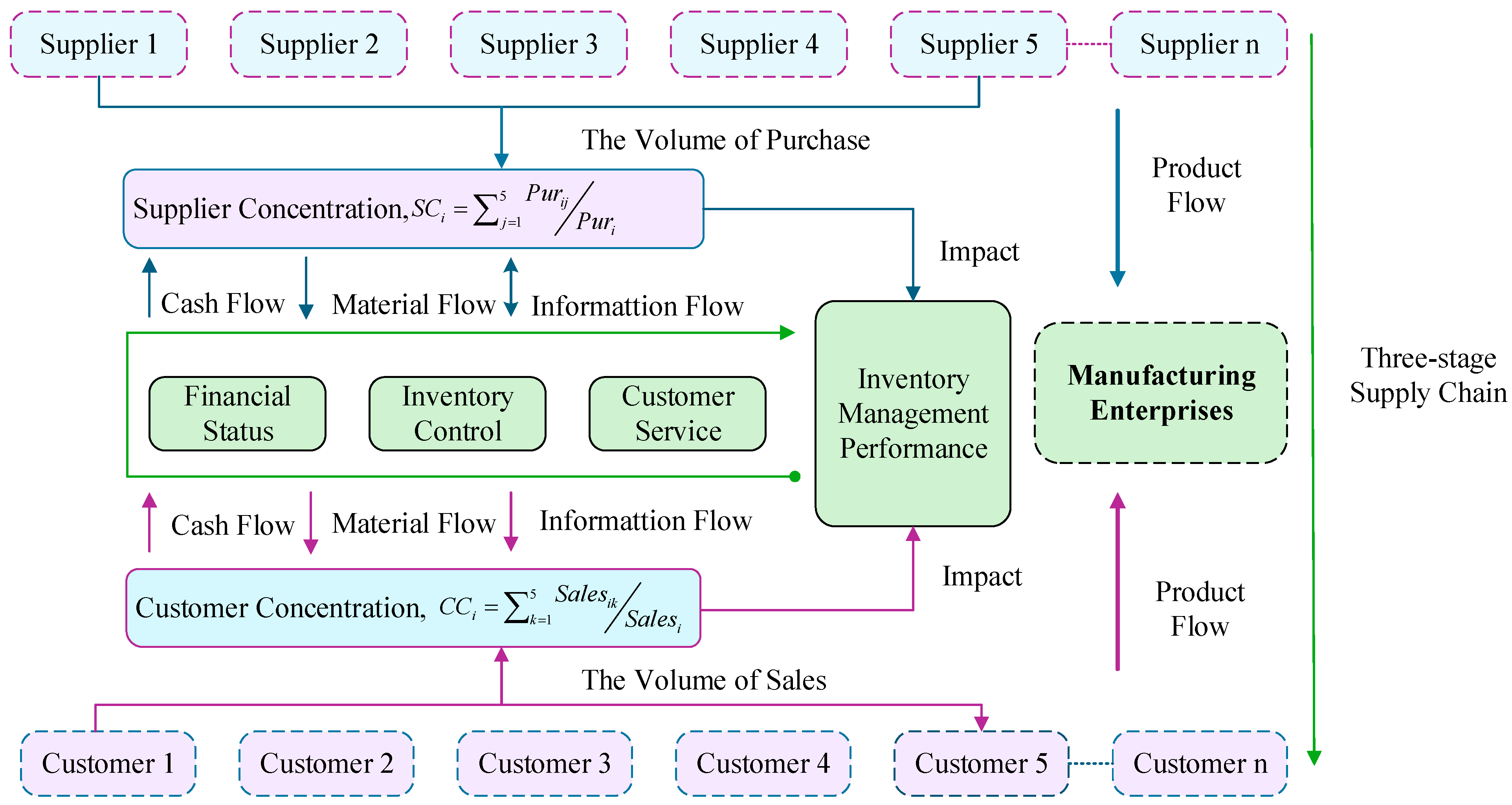
Prior to analysis, all indicator values were normalized to a [0, 1] range, using the extreme value method to minimize the impact of extreme values. The entropy values, difference coefficients and final weights for each indicator were then systematically computed. The resulting dimension weights are as follows: inventory control quality at 40.97%, financial performance at 39.80% and customer service level at 19.23%. The reasonableness of this weighting scheme was verified through sensitivity analysis, which incorporated a Monte Carlo simulation and subsystem contribution assessment in Figure 1.

3.1.3. Interaction Between SCC and IMP

This study models the interaction between the SCC and IMP as a feedback loop from a three-stage supply chain [32,33]. Figure 2 is a system dynamics diagram showing how the SCC exerts two counter effects on IMP at the same time. A better SC optimizes the efficiency of the interaction with key partners [34]. Thus, this optimization will flatten the material flow and perhaps reduce the level of finished goods inventory.

In the model formulation, SC directly controls information and financial flows, while SC controls logistics through intermediate information flows [35]. In contrast, high CC creates the demand for forecast complexity and hence, requires higher safety levels. It also reduces manufacturers’ bargaining power and margin flexibility [36]. More importantly, there are even two interacting loops in this relationship. Although high SCC may be a potential threat to the robustness of the whole supply chain [37], high IMP provides slack in operation and financial flexibility that allows the supplier and customer base to pursue strategic diversification paths. Therefore, the reverse causality relationship exists as a coevolutionary mechanism in which the network structure and operation performance adjust to each other over time. The SD methodology explores how the SCC and IMP reciprocally influence each other under different operational conditions and time horizons.

3.2. Construction of System Dynamics Model

3.2.1. Fundamental Assumptions

To clarify the research range and be consistent with the related modeling conventions, the SD model in this study about the relationship between the SCC and IMP has the following assumptions:

(1)

The model is treated as one kind of product converted from one kind of raw materials. The multiple materials situations can be decomposed into multi-BOMs and multi-sourcing strategies. The model is considered to be a product that is converted out of a single type of raw material. By this simplification, we can easily isolate the effects of SCC on inventory management without complicating the relationships with interactions with the multi-product, which can confound causal relationships. The multi-product situation would also be resolved in future research through the breakdown of the latter into multi-BOMs and multi-sourcing [38].

(2)

The possible decrease in demand can be avoided by early warnings and adjustable production strategies. It is assumed that the demand for products in the market will grow consistently with time. This assumption is differentiated by the trends in historical demands of the furniture producing business and guarantees model stability. It allows the simulation to replicate the effects of the SCC on IMP in normal operation conditions, and the effect of the sudden market shocks is not considered. In extended studies, a scenario analysis of the demand change can be implemented [24].

(3)

The model fails to consider such extreme situations as natural calamities or epidemics. It is concerned with the study of normal operation conditions and inherent feedback requirements between the SCC and IMP. Stochastic modeling would entail additional inclusion of extreme events, which are not within the borders of the current study [28].

(4)

The manufacturing enterprise communicates with upstream raw material suppliers and downstream customers, and the whole chain has a three-stage structure. The supply chain is presented in the form of a three-stage system, which includes upstream suppliers, manufacturers and downstream customers. Such a structure is reminiscent of the common countenance in the target industry, permitting the model to capture the major details and material and financial shifts and retain computational triviality. It also maintains the crucial feedback processes that are needed to investigate the coevolutionary processes between the SCC and IMP [39].

(5)

There is no significant regulatory or contractual anomaly in the operation of all enterprises and supply chain partners. The first assumption is that the modeled relationships will imply typical patterns of operations; the results of the simulation are more generalized in the framework of the manufacturing sphere [18].

(6)

The initial conditions of the system variables, such as a level of inventory, work-in-process and total business, are established through the historical data of the chosen Chinese manufacturers. This makes the model begin with real-world conditions and enables the findings to be produced by observations to be empirically checked against the results [11].

3.2.2. Model Parameters

The SD simulation requires a platform that supports transparent equation inspection, reliable continuous time computation and a clear construction of causal loop and stock and flow structures. Such features are essential for academic model validation and are not equally supported by other commercial SD tools, such as Stella or Powersim [30]. Therefore, Vensim PLE (Version 7.3.5, Ventana Systems, Inc., Harvard, MA, USA) is employed, because it provides a stable, rigorously validated modeling environment that is widely recognized in system dynamics studies. The SD model was coded and simulated with the Vensim PLE 7.3.5 program. The values of the parameters were established by using empirical studies, industry reports and historical data from manufacturers to represent the normally experienced opera-operational conditions. All the parameters of

Table 2. Key constants, set in the SD model of SCC and IMP.

Constants	Symbols	Values	Units	Bibliographic Support
Supplier Concentration	$\mathrm{SC}$	Simulation Settings	Dmnl	[18]
Customer Concentration	$\mathrm{CC}$	Simulation Settings	Dmnl	[17]
Initial In-Transit Inventory	$\mathrm{IITS}$	100,000	Pcs	[27]
Initial Work in Process	$\mathrm{IWIP}$	50,000	Pcs	[27]
Initial Inventory	$\mathrm{I}{\mathrm{I}}_{\mathrm{t}}$	120,000	Pcs	[27]
Linear Initial Demand	$\mathrm{Drp}$	75,000	Pcs	[27]
Set-Up Order Cost	$\mathrm{FC}$	100	Dmnl	[23]
Holding Cost Per Unit	$\mathrm{h}$	0.32	Dmnl	[27]
Delivery Delay	$\mathrm{Dd}$	1	week	[6]
Transportation Delay	$\mathrm{Td}$	2	week	[23]
Production Delay	$\mathrm{Pd}$	1	week	[23]
Thresholds for Supply Chain Stability	$\mathrm{Tscs}$	0.1	Dmnl	[9]
Raw Material Benchmark Prices	$\mathrm{Prm}$	9	Dmnl	[23]
Demand Forecast Benchmark	$\mathrm{Dfb}$	1	Dmnl	[27]
Maximum Price of Raw Materials	${\mathrm{Prm}}_{\max }$	9.5	Dmnl	[23]
Lowest Price for Raw Materials	${\mathrm{Prm}}_{\min }$	8.3	Dmnl	[23]
Product Benchmark Price	$\mathrm{Pm}$	18.5	Dmnl	[11]
Maximum Price of the Product	${\mathrm{Pm}}_{\max }$	20	Dmnl	[17]
Lowest Price for the Product	${\mathrm{Pm}}_{\min }$	17.5	Dmnl	[17]
Customer Churn Threshold	$\mathrm{Tcsi}$	0.9	Dmnl	[36]
Customer Churn	$\mathrm{Mac}$	0.5	Dmnl	[36]
Proportion of the Financial Performance	$\mathsf{\alpha }$	0.3	Dmnl	[11]
Proportion of Inventory Control	$\mathsf{\beta }$	0.4	Dmnl	[8]
Proportion of Customer Service	$\mathsf{\gamma }$	0.3	Dmnl	[8]
Impact Factor of SCC	$\mathrm{IFsc}$	0.38	Dmnl	[9]
Impact Factor of Operational Efficiency	$\mathrm{IFoe}$	1.125	Dmnl	[8]
Inventory Adjustments Coefficient	$\mathrm{IAC}$	1	Dmnl	[11]
Distributed Demand Coefficient	$\mathrm{Ddc}$	0.2	Dmnl	[9]

have a reference to where they were obtained, so there is full reproducibility of the model.

3.2.3. Causal Loop Diagram and Stock and Flow Diagram

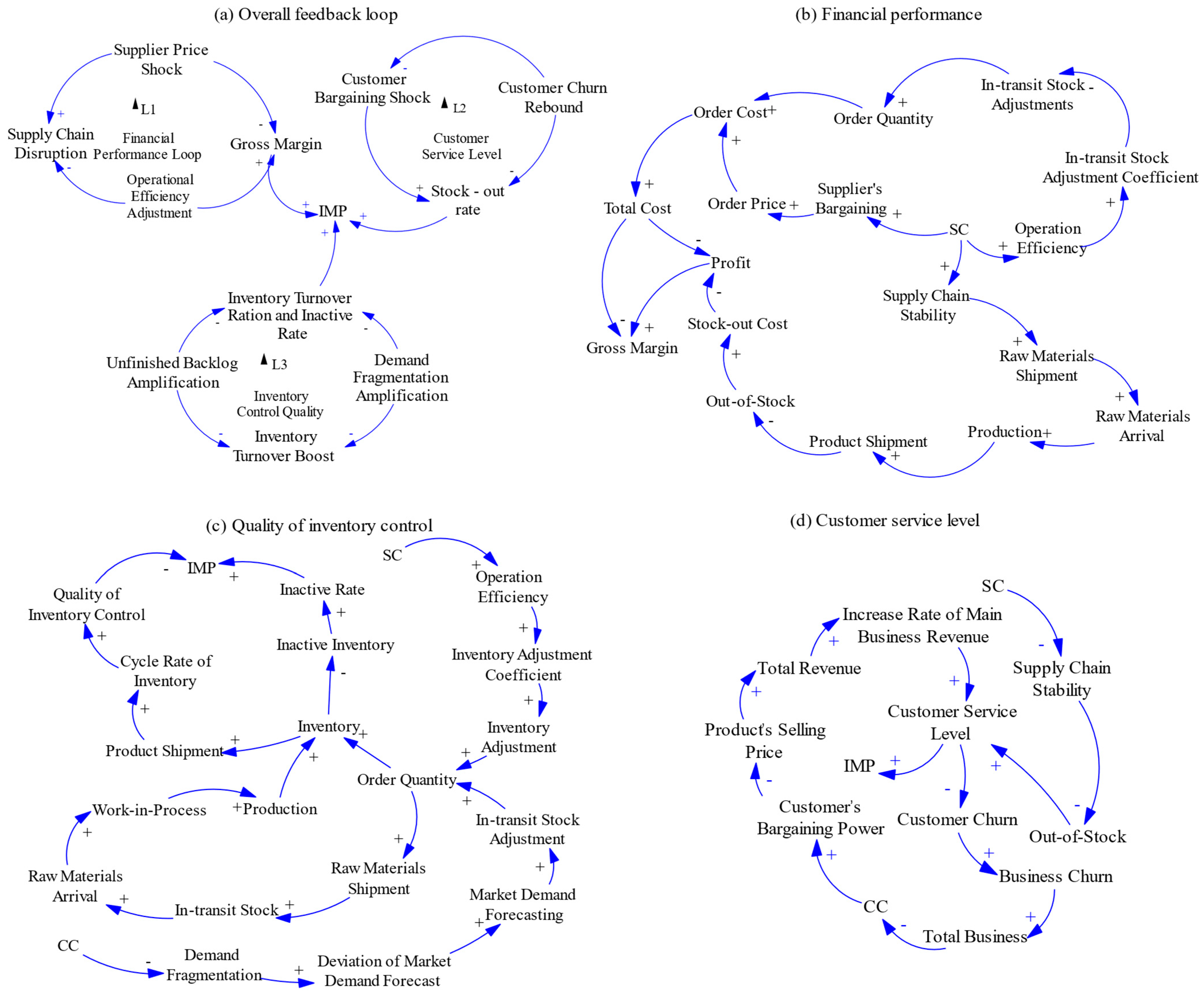
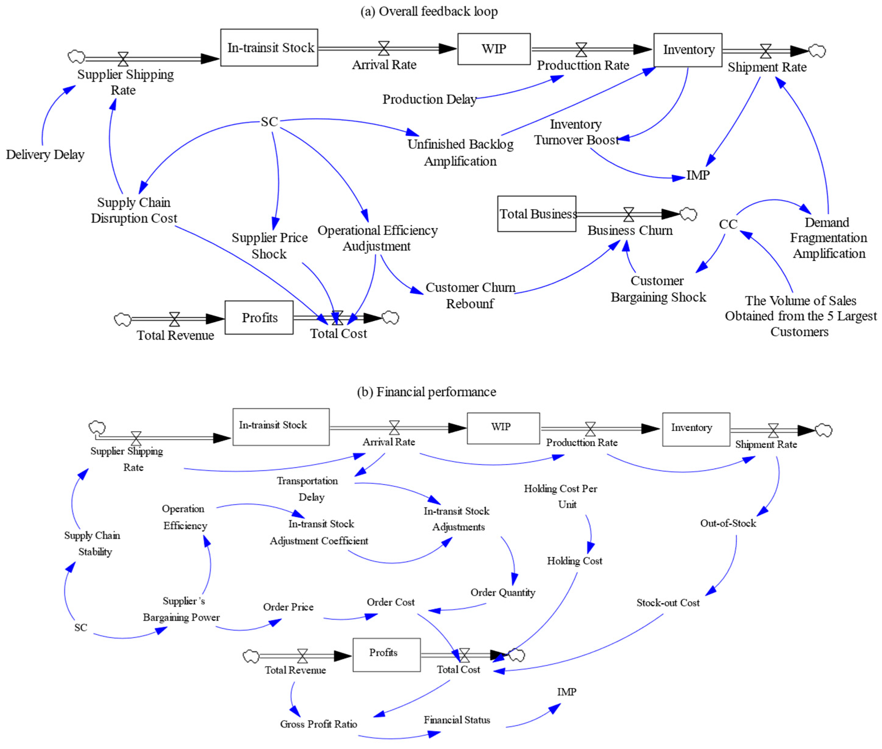
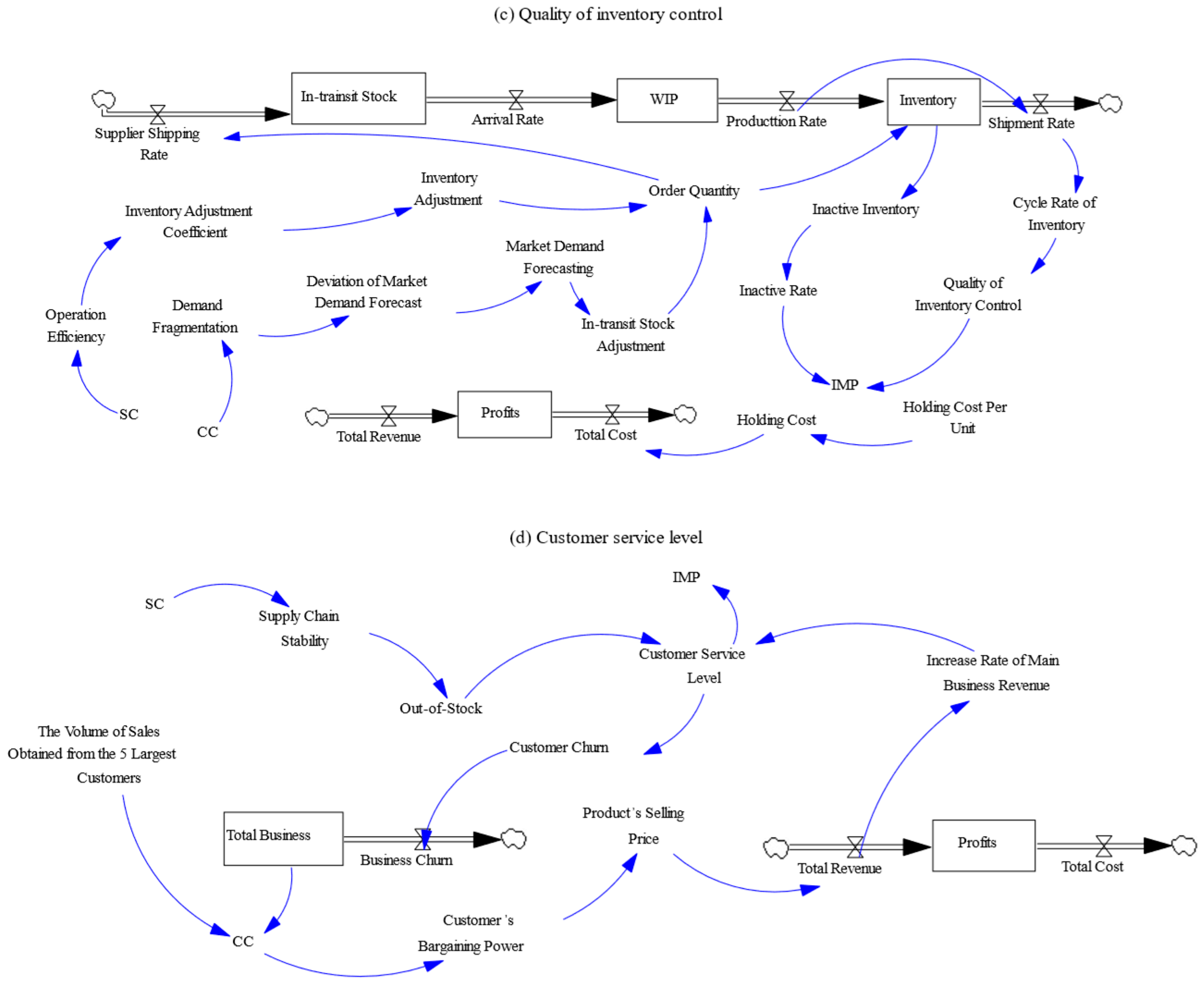
The causal loop diagram (CLD) shows the feedback loops that maintain the system’s behavior in a certain way (polarity signs). A polarity sign of “+” for a loop means that the two variables in the loop have the same reinforcing feedback relationship: both variables move in the same direction. A polarity sign of “–“ for a loop means that the two variables have an inverse relationship: one variable moves in the opposite direction to the other. There are eight feedback paths in total, categorized by the three dimensions of IMP. The pathways between variables are fully detailed in Appendix A. Paths 1–3 affect the gross margin through different mechanisms (Figure 3b), whereas Paths 4–6 affect the inventory control quality (Figure 3c) and Paths 7 and 8 affect the customer service level (Figure 3d). These feedback paths are generalized into an integrated view in Figure 3a.

Paths 1–3 affect the gross margin through different mechanisms. Path 1 connects the SC to the supplier’s bargaining power, which has a direct effect on the order price and procurement cost and, consequently, affects the gross margin [12]. In the global NAND Flash market, a 12% change in the ordering cost is found to affect the gross margin by 3.2% on average [40]. Path 2 goes from the SC to the gross margin, via the gross margin. When supply stability is small, the production throughput and distribution are affected by the supply stability, and the frequency of stock outings rises, which results in poor financial performance. For instance, when Typhoon Doksuri occurred in 2023, production and distribution were affected, and the gross margin dropped by 2.1%. Path 3 shows the effect of the SC on the gross margin via transit inventory efficiency. When the efficiency of the transit inventory improves, the work-in-process inventory decreases, and the ordering cycle is ideal [41]. When a manufacturing execution system was introduced into our company, the gross margin increased by 3%, due to better operational performance caused by the high efficiency of the transit inventory [42].

Paths 4–6 affect the inventory control quality. Path 4 takes turnover as an indicator of performance. The implementation of RFID in Inditex improved the turnover from 4.2% to 6.1% and reduced the proportion of slow-selling items by 20% [43]. Path 5 introduces the inventory adjustment coefficient as a stabilizing factor in negative feedback loops. When the inventory adjustment coefficient was improved with the help of AI adjustment, the number of backorders was reduced by 12% and the backlog rate was reduced from 9.2% to 8.5% [44]. Path 6 shows the adverse effect of demand fragmentation on demand forecasting as its starting point. With the help of AI forecasting, forecast errors have been reduced from 30% to 11% [45]. Meanwhile, the practice of synchronized replenishment improved inventory turnover by 25% [46].

Paths 7 and 8 are related to customers. The high CC increases the bargaining power of the buyer. In return, this increases pricing pressure and reduces revenue [47]. The results of the empirical analysis show that higher bargaining power of the buyer is significantly related to margin erosion [48]. Path 8 shows that supply disruption increases the probability of stock-out. Stock-outs impact service quality and cause churn of customers [49]. Churn increases the CC and causes dependency on key customers.

Although the CLD clearly shows the qualitative structure of the system and the nature of the feedback relationships within it, it cannot show the quantitative relationships between variables. We therefore introduce the stock and flow diagram, which uses two kinds of variables: flows, which show rates of change over time, and stocks, which show an accumulated state. In our model, four example stock variables are in-transit stock, work in process (WIP), inventory, total business and profits. In-transit stock is the number of materials or parts that have left the warehouse of their supplier but are now not at the location of the manufacturer. It stores the flow of the “raw material delivery rate” and empties it through the flow of the raw material receipt rate. Coordinating focus on these stocks is consonant with established inventory theory, which states that integrated control of these variables benefits IMP [50,51]. The full stock and flow diagram is shown in Figure 4.

3.2.4. Main Equations

Parametric equation determination is the next major step in the SD method. Each variable in the model is defined by a mathematical relationship to other variables. There are three types of relationships: level, rate or auxiliary. Level variables are the system inventories or amounts accumulated over time. They are the variables that “build up” over time. Each represents the accumulation of its previous value and its net change over each time step. Rate variables are the flows into or out of inventories, and their values directly determine the inflows and outflows that drive stock adjustments. Auxiliary variables are computed from other variables but are not themselves accumulations. The main variables and equations of the SD model are summarized in

Table 3. Variables and equations for the IMP SD model under the SCC.

The Type of Variable	Variables	Symbols	Equations	Serial Number
Level	In-Transit Stock	$\mathrm{ITS}$	$\mathrm{ITS}=\mathrm{INTEG}({\mathrm{Dss}}_{\mathrm{t}}-{\mathrm{A}}_{\mathrm{t}},\mathrm{IITS})$	(6)
	Work In Process	$\mathrm{WIP}$	$\mathrm{WIP}=\mathrm{INTEG}({\mathrm{A}}_{\mathrm{t}}-{\mathrm{Dp}}_{\mathrm{t}},\mathrm{IWIP})$	(7)
	Inventory	${\mathrm{I}}_{\mathrm{t}}$	${\mathrm{I}}_{\mathrm{t}}=\mathrm{INTEG}({\mathrm{Dp}}_{\mathrm{t}}-\mathrm{Ds},\mathrm{I}{\mathrm{I}}_{\mathrm{t}})$	(8)
	Profits	$\mathrm{Pr}$	$\mathrm{Pr}=\mathrm{INTEG}(\mathrm{Tr} -\mathrm{Tc},\mathrm{IPr})$	(9)
	Total Business	$\mathrm{Tb}$	$\mathrm{Tb}=\mathrm{INTEG}(-\mathrm{Bc},\mathrm{ITb})$	(10)
Rate	Raw Materials Shipment	${\mathrm{Dss}}_{\mathrm{t}}$	${\mathrm{Dss}}_{\mathrm{t}}=\mathrm{IF} \mathrm{THEN} \mathrm{ELSE}(\mathrm{Scs} \le \mathrm{Tscs}, 0,$ $\mathrm{DELAY}1({\mathrm{O}}_{\mathrm{t}},\mathrm{Dd}\left)\right)$	(11)
	Raw Materials Arrival	${\mathrm{A}}_{\mathrm{t}}$	${\mathrm{A}}_{\mathrm{t}}=\mathrm{DELAY}1({\mathrm{Dss}}_{\mathrm{t}},\mathrm{Td})$	(12)
	Production	${\mathrm{Dp}}_{\mathrm{t}}$	${\mathrm{Dp}}_{\mathrm{t}}=\mathrm{DELAY}1({\mathrm{A}}_{\mathrm{t}},\mathrm{Pd})$	(13)
	Product Shipment	$\mathrm{Ds}$	$\mathrm{Ds} = \mathrm{MAX}(0,\mathrm{MIN}(\mathrm{Dr} (\mathrm{or} \mathrm{Dl}),{\mathrm{I}}_{\mathrm{t}})$)	(14)
	Total Cost	$\mathrm{Tc}$	$\mathrm{Tc}=\mathrm{Ih}+{\mathrm{Sc}}_{\mathrm{t}}+{\mathrm{OC}}_{\mathrm{t}}$	(15)
	Total Revenue	$\mathrm{Tr}$	$\mathrm{Tr}=\mathrm{Ds} \times \mathrm{p}$	(16)
	Business Churn	$\mathrm{Bc}$	$\mathrm{Bc}=\mathrm{Ac}$	(17)
Auxiliary	Suppliers’ Bargaining Power	$\mathrm{Psb}$	$\mathrm{Psb}=\mathrm{SC}$	(18)
	Customers’ Bargaining Power	Pcb	$\mathrm{Pcb}=\mathrm{CC}$	(19)
	Order Price	$\mathrm{w}$	$\mathrm{w}=\mathrm{Prm}+\mathrm{Psb} \times \left({\mathrm{Prm}}_{\max }-\mathrm{Prm}\right)-\left(1 -\mathrm{Psb}\right)$ $\times (\mathrm{Prm} -{\mathrm{Prm}}_{\min })$	(20)
	Selling Price Per Unit	$\mathrm{p}$	$\mathrm{p}=\mathrm{Pm} -\mathrm{Pcb} \times \left({\mathrm{Pm}}_{\max }-\mathrm{Pm}\right)+(1$ $-\mathrm{Pcb}) \times (\mathrm{Pm}-{\mathrm{Pm}}_{\min })$	(21)
	Order Quantity	${\mathrm{O}}_{\mathrm{t}}$	${\mathrm{O}}_{\mathrm{t}}=\mathrm{Max}(0,{\mathrm{D}}_{\mathrm{t}}+{\mathrm{ITSA}}_{\mathrm{t}}+{\mathrm{IA}}_{\mathrm{t}})$	(22)
	Order Cost	${\mathrm{OC}}_{\mathrm{t}}$	${\mathrm{OC}}_{\mathrm{t}}=\mathrm{IF} \mathrm{THEN} \mathrm{ELSE}({\mathrm{O}}_{\mathrm{t}}=0,0,\mathrm{FC}+\mathrm{w} \times {\mathrm{O}}_{\mathrm{t}})$	(23)
	Holding Cost	$\mathrm{Ih}$	$\mathrm{Ih}=\mathrm{h} \times {\mathrm{I}}_{\mathrm{t}}$	(24)
	Stock-Out Cost	${\mathrm{Sc}}_{\mathrm{t}}$	${\mathrm{Sc}}_{\mathrm{t}}=(\mathrm{p} -\mathrm{w}) \times (\mathrm{Dr} \mathrm{or} \mathrm{Dl}-\mathrm{Ds})$	(25)
	Cycle Rate of Inventory	$\mathrm{Cri}$	$\mathrm{Cri}=\mathrm{Ds}/{\mathrm{I}}_{\mathrm{t}}$	(26)
	Customer Churn	$\mathrm{Ac}$	$\mathrm{Ac}=\mathrm{IF} \mathrm{THEN} \mathrm{ELSE}\left(\right(1-\mathrm{Sor}) \le \mathrm{Tcsi},\mathrm{Mac},0)$	(27)
	Stock-Out Rate	$\mathrm{Sor}$	$\mathrm{Sor}=\mathrm{Os}/\mathrm{Dr}(\mathrm{or} \mathrm{Dl})$	(28)
	Inventory Management Performance	$\mathrm{IMP}$	$\mathrm{IMP}=\mathsf{\alpha } \times \mathrm{Fs}+ \mathsf{\beta } \times \mathrm{Ic}+\mathsf{\gamma } \times \mathrm{Cs}$	(29)
	Operation Efficiency	$\mathrm{Oe}$	$\mathrm{Oe}=\mathrm{IFsc} \times \mathrm{SC}$	(30)
	In-Transit Stock Adjustment	${\mathrm{ITSA}}_{\mathrm{t}}$	${\mathrm{ITSA}}_{\mathrm{t}}=\mathrm{ITSAC} \times (\mathrm{Td} \times { \mathrm{D}}_{\mathrm{t}}-\mathrm{ITS})$	(31)
	In-Transit Stock Adjustment Coefficient	$\mathrm{ITSAC}$	$\mathrm{ITSAC}=\mathrm{IFoe} \times \mathrm{Oe}$	(32)
	Inventory Adjustment	${\mathrm{IA}}_{\mathrm{t}}$	${\mathrm{IA}}_{\mathrm{t}}=\mathrm{IAC} \times ({\mathrm{D}}_{\mathrm{t}}-{\mathrm{I}}_{\mathrm{t}})$	(33)
	Market Demand Forecasting	${\mathrm{D}}_{\mathrm{t}}$	${\mathrm{D}}_{\mathrm{t}}=\mathrm{SMOOTH}(\mathrm{Ds},{\mathrm{T}}_{\mathrm{a}}) \times { \mathrm{D}}_{\mathrm{b}}$	(34)
	Deviation of the Market Demand Forecast	${\mathrm{D}}_{\mathrm{b}}$	${\mathrm{D}}_{\mathrm{b}}=\mathrm{Dfb}+\mathrm{Df} \times \mathrm{Ddc}$	(35)
	Demand Fragmentation	$\mathrm{Df}$	$\mathrm{Df}=(\mathrm{Sales}-{\sum }_{\mathrm{j}=1}^5{\mathrm{Sales}}_{\mathrm{j}})/\mathrm{Sales}$	(36)
	Linear Demand	$\mathrm{Dl}$	$\mathrm{Dl}=(\mathrm{Drp} +\mathrm{Time} \times \mathrm{d}) \times (\mathrm{Tb}/10)$	(37)
	Random Demand	$\mathrm{Dr}$	$\mathrm{Dr}=\left(\mathrm{Da}+\mathrm{RANDOM} \left(\mathrm{a},\mathrm{b}, \mathrm{c} \right)\right) \times (\mathrm{Tb}/10)$	(38)
	Financial Performance	$\mathrm{Fp}$	$\mathrm{Fp}=\left(\mathrm{Tr}-\mathrm{Tc}\right)/\mathrm{Tr}$	(39)
	Inactive Rate	$\mathrm{Ir}$	$\mathrm{Ir}=\mathrm{Sp}/{\mathrm{I}}_{\mathrm{t}}$	(40)
	Increase Rate of Main Business Revenue	$\mathrm{Ibr}$	$\mathrm{Ibr}={(\mathrm{Tr}}_{\mathrm{t}}-{\mathrm{Tr}}_{\mathrm{t}-1})/{\mathrm{Tr}}_{\mathrm{t}-1}$	(41)
	Inventory Control	$\mathrm{Ic}$	$\mathrm{Ic}=\mathrm{Cri}/2+\mathrm{Ir}/2$	(42)
	Customer Service	$\mathrm{Cs}$	$\mathrm{Cs}=(1-\mathrm{Sor}) \times (2/3)+\mathrm{Ibr} \times (1/3)$	(43)
	Out-of-Stock	$\mathrm{Os}$	$\mathrm{Max}(0,\mathrm{Dr}(\mathrm{or} \mathrm{Dl})-\mathrm{Ds})$	(44)
	Inactive Inventory	$\mathrm{Sp}$	$\mathrm{Sp} = \mathrm{Max}(0,{\mathrm{I}}_{\mathrm{t}} - \mathrm{Dl} (\mathrm{or} \mathrm{Dr}))$)	(45)
	Supply Chain Stability	Scs	$\mathrm{Scs}=1-\mathrm{SC}$	(46)

[27,31,41].

Each functional relationship is designed so its logic is clear and can be reproduced. Stock variables use integrated formulations to take into consideration the state of natural accretion of material and monetary values. The rates of the materials are based on first-order delay structures that describe sequential processing steps and transportation steps of manufacturing systems. Inventory and in-transit corrections are based on proportional response theory, which is in line with classical system dynamics inventory control theory. Maximum, minimum and conditional functions are used to provide nonlinear expressions to model the effect of capacity limits, stock-out situations and bargaining effects under operational constraints. Demand forecasting is a combination of smoothing and random disturbances and considers both predictable and market uncertainty, which means the behavior of the model in response to disturbances is realistic.

In this study, we adopt the SCC as a proxy variable of bargaining power. It is assumed that an increase in the concentration would make manufacturers more dependent on their suppliers and customers and thus decrease their bargaining power [8]. However, it should be noted that concentration is only one of the factors that affect the bargaining power. In general, the SD approach is an appropriate analytical tool to use in the current study, in that it can capture the dynamic interaction and feedback loops included in supply chain management systems.

4. SD Model Validation

The model is considered to be valid when the deviation between simulated outputs and historical data remains within 10%. This study selects TIANCI and SOGAL for validation, due to their stable operations and significant market presence, which are representative for analyzing how supply SCC affects IMP. Based on their distinct data characteristics and customer industry profiles, the two enterprises are categorized into linear and random demand patterns. This methodological framework, however, can also be applied to other enterprises. However, it too has some limitations on its applicability. More specifically, the model assumes relatively steady production cycles, indicators of concentration that are measurable and consistent inventory accounting approaches. Model performance can be limited in other situations where the businesses are operating in a very dynamic environment, where reliable data are not available and in businesses where unconventional patterns of supply chain arrangement are in use.

4.1. Model Validation Under Linear Growth Demand Pattern

TIANCI has been the world’s leading electrolyte manufacturer since 2017. In recent years, the expansion of the new energy vehicle industry has caused a shortage of lithium hexafluorophosphate, which is the core material for electrolytes. Based on the variation in monthly sales volume from 2013 to 2022, derived from the latest publicly available data, the actual market demand of TIANCI is defined as a linear growth pattern, according to Equation (33).

The SD model of TIANCI is simulated using Vensim PLE, with initial operating data from the 2013–2022 period in

Table 4. The data from TIANCI, imported into the SD model.

Year	SC (%)	CC (%)	Raw Material Cost Per Unit (CNY)	Selling Price Per Unit (CNY)	Product Cost Per Unit (CNY)	Initial Demand (ton)	Added Demand (ton)
2013	30.89	22.83	8473.18	16,148.55	10,678.93	630.00	3.44
2014	30.32	21.28	7287.50	13,454.96	9324.50	770.71	9.85
2015	21.60	30.05	7827.37	14,126.50	9693.11	899.70	15.18
2016	39.31	37.76	10,500.02	20,635.68	12,492.39	1284.46	16.12
2017	33.31	37.74	10,704.31	19,567.56	12,834.61	1492.77	20.94
2018	31.56	38.38	10,357.13	16,633.85	12,495.43	2078.14	13.24
2019	31.56	41.99	10,146.35	17,991.49	13,347.21	2380.79	21.94
2020	37.14	43.47	9981.36	21,556.31	13,787.31	2067.24	64.18
2021	33.89	66.89	18,506.59	34,491.90	22,345.81	3642.09	98.59
2022	36.86	70.82	17,432.73	34,853.66	22,757.43	3465.73	87.46

Data resource: The data can be obtained from the Foresight Database (https://d.qianzhan.com/) and the Juchao Information Network (http://www.cninfo.com.cn/new/index) (accessed on 23 August 2025).

. The SC and CC values are obtained directly from the enterprise’s annual reports. The raw material cost and unit selling price are calculated based on manufacturing revenue and sales volume data. Detailed data from the 2013–2022 annual reports are provided in Appendix B, while TIANCI’s monthly sales volumes from 2015 to 2022 are included in Appendix C. The simulated IMP results are presented in

Table 5. Simulated values’ IMP of TIANCI from 2013 to 2022.

Year	Simulated Value	Year	Simulated Value
2013	0.6964	2018	0.6947
2014	0.6937	2019	0.6982
2015	0.6825	2020	0.7265
2016	0.7109	2021	0.7453
2017	0.7023	2022	0.7396

.

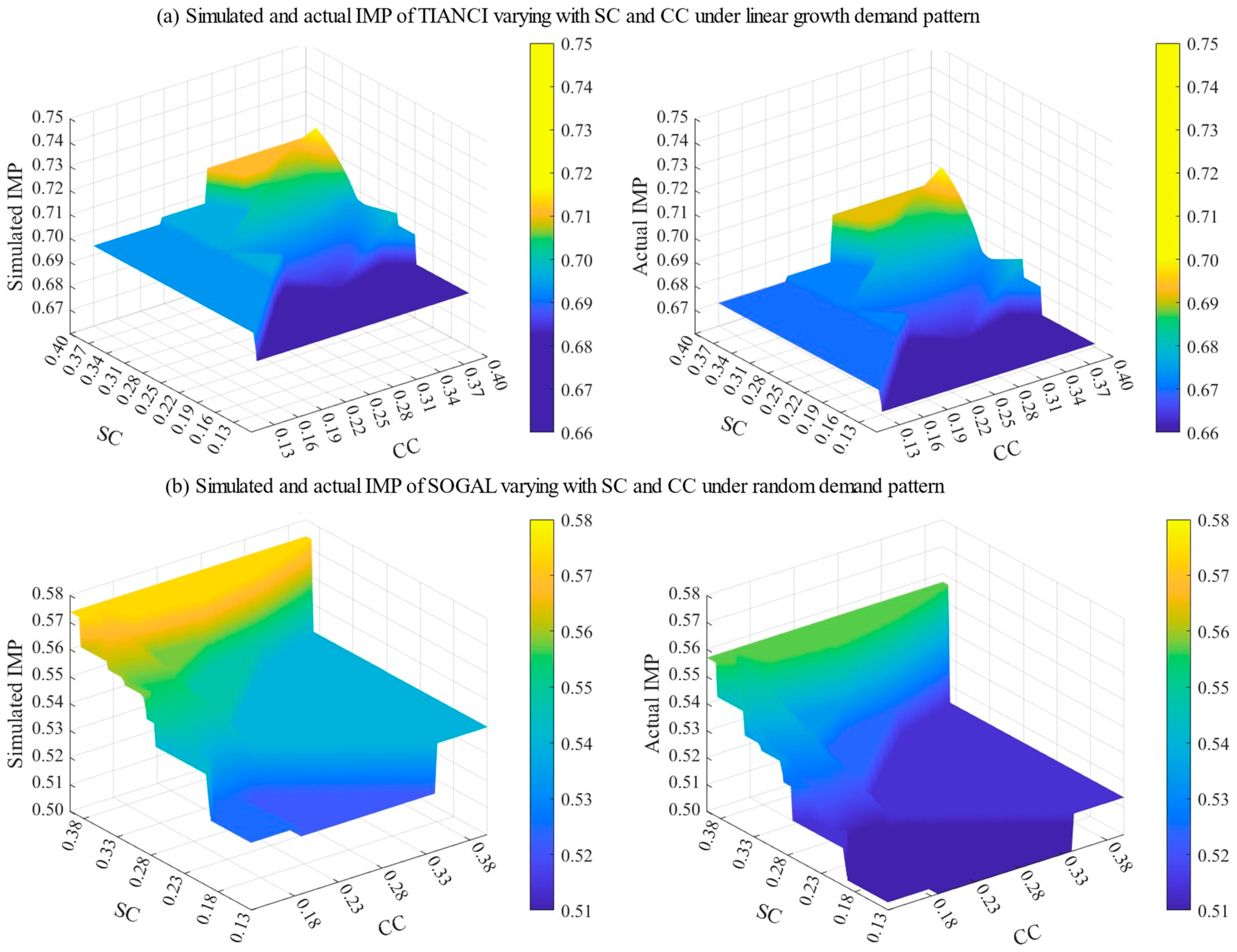
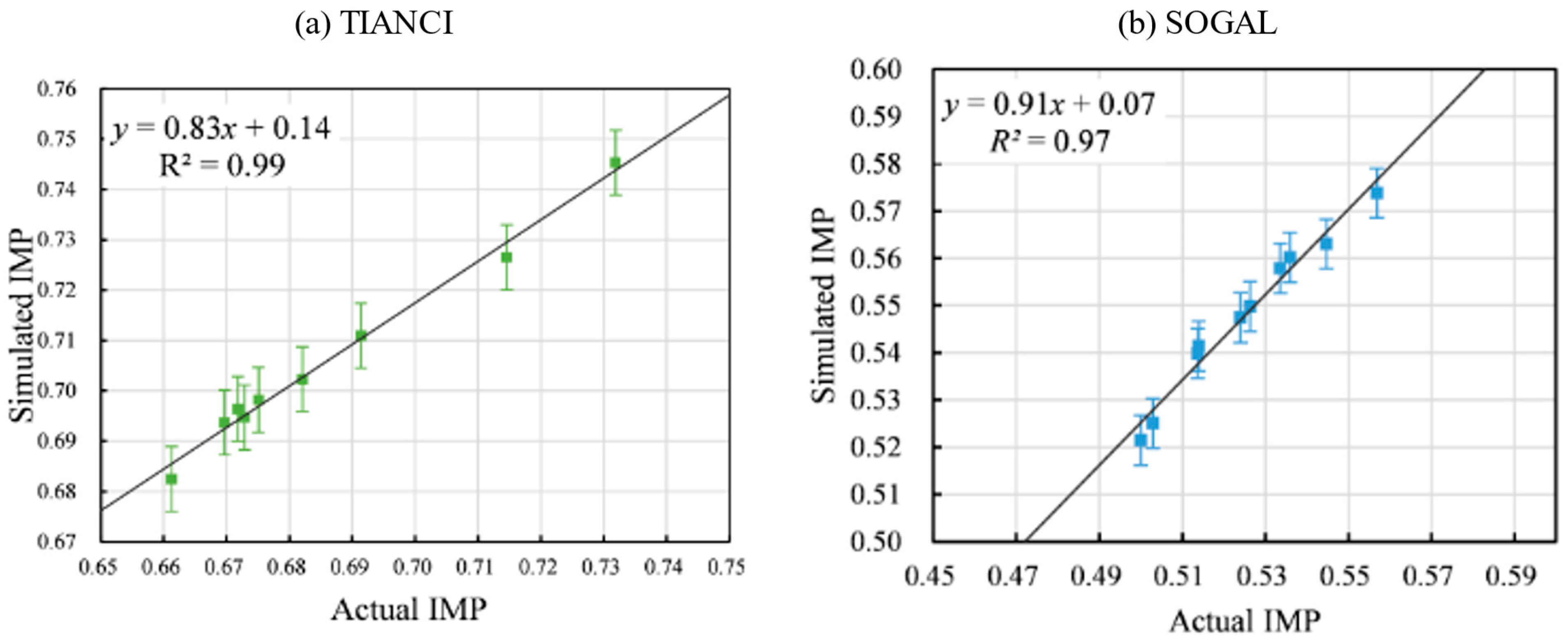
Based on the simulated IMP output under TIANCI’s linear demand pattern, the historical data test results show strong model validity. First, Figure 5a presents the surface plots of both simulated and actual IMP, demonstrating that the change in simulated IMP with SC and CC is highly consistent with the actual IMP in the three-dimensional surface plot. Second, a clear linear relationship between actual and simulated IMP in Figure 6a confirms that the SD model achieves high accuracy in simulated IMP. The actual IMP values are computed from the Appendix B data. Finally, as shown in

Table 6. Historical test of IMP-related data for TINCI from 2013 to 2022.

Year	SC (%)	CC (%)	IMP
			Actual Value	Simulated Value	Relative Error
2013	30.89	22.83	0.6718	0.6964	0.0366
2014	30.32	21.28	0.6697	0.6937	0.0358
2015	21.60	30.05	0.6613	0.6825	0.0321
2016	39.31	37.76	0.6914	0.7109	0.0282
2017	33.31	37.74	0.6821	0.7023	0.0296
2018	31.56	38.38	0.6729	0.6947	0.0324
2019	31.56	41.99	0.6751	0.6982	0.0342
2020	37.14	43.47	0.7146	0.7265	0.0167
2021	33.89	66.89	0.7319	0.7453	0.0183
2022	36.86	70.82	0.7239	0.7396	0.0217

, the relative error of the model remains less than 10%, meeting the error standard specified in this study. These comprehensive results confirm that the SD model has successfully passed the historical data test.

4.2. Model Validation Under Random Demand Pattern

SOGAL operates as a custom furniture enterprise, specializing in the research, development, production and sale of furniture products. Based on variations in its monthly sales volume, the actual market demand for SOGAL is characterized as following a random demand pattern.

For model validation, monthly sales data for SOGAL from 2012 to 2021 are provided in Appendix D, while the corresponding annual report data used to obtain the SC, CC and product selling price are presented in Appendix E. The SC and CC are directly extracted from these reports, while the order price and unit selling price are calculated based on the reported financial data. The average, maximum and minimum demand values are derived from monthly sales volumes, with specific parameter settings provided in

Table 7. Data from SOGAL, imported into the SD Model.

Year	SC (%)	CC (%)	Order Price (CNY)	Selling Price Per Unit (CNY)	Average Demand (m2)	Maximum Demand (m2)	Minimum Demand (m2)
2013	0.394	0.158	104.53	167.22	373,836	469,274	327,479
2014	0.354	0.134	100.40	159.37	397,737	473,997	337,758
2015	0.329	0.149	91.09	146.71	416,338	484,284	340,523
2016	0.274	0.180	98.87	155.46	557,408	660,819	421,209
2017	0.237	0.211	107.77	173.95	675,967	895,512	534,418
2018	0.218	0.198	111.11	177.96	785,221	1,051,149	636,552
2019	0.232	0.148	119.32	189.97	773,833	997,886	583,669
2020	0.217	0.166	131.71	208.27	767,900	1,120,094	286,708
2021	0.276	0.175	144.03	216.72	917,787	1,142,904	701,328
2022	0.231	0.132	139.27	225.31	872,473	1,097,427	694,737

Data resource: The data can be obtained from the Foresight Database (https://d.qianzhan.com/) and the Juchao Information Network (http://www.cninfo.com.cn/new/index) (accessed on 2 October 2025).

. The simulated IMP output is summarized in

Table 8. Simulated values for IMP of SOGAL from 2013 to 2022.

Year	Simulated Value	Year	Simulated Value
2013	0.5738	2018	0.5214
2014	0.5630	2019	0.5414
2015	0.5579	2020	0.5250
2016	0.5474	2021	0.5498
2017	0.5398	2022	0.5387

.

The historical data test results, based on the simulated IMP, are as follows. First, Figure 5b displays the surface plots of both simulated and actual IMP, showing that the simulated IMP varies with SC and CC, in close agreement with the actual IMP in the three-dimensional representation. Second, a strong linear relationship between the actual and simulated IMP is observed in Figure 6b, with a coefficient of determination (R²) of 0.97, indicating high simulation accuracy. Finally,

Table 9. Historical test of IMP-related data for SOGAL from 2013 to 2022.

Year	SC (%)	CC (%)	IMP
			Actual Value	Simulated Value	Relative Error
2013	39.40	15.80	0.5569	0.5738	0.0303
2014	35.45	13.44	0.5447	0.5630	0.0336
2015	32.96	14.97	0.5336	0.5579	0.0455
2016	27.45	18.07	0.5240	0.5474	0.0446
2017	23.79	21.19	0.5137	0.5398	0.0509
2018	21.88	19.80	0.5000	0.5214	0.0429
2019	23.26	14.82	0.5140	0.5414	0.0534
2020	21.73	16.66	0.5029	0.5250	0.0440
2021	27.57	17.52	0.5263	0.5498	0.0447
2022	23.08	13.39	0.5172	0.5390	0.0422

compares the simulated and actual IMP values from 2013 to 2022. The relative error of the model remains within the predefined acceptable range, confirming that the SD model has successfully passed the historical data test.

5. Simulation Results and Discussion

5.1. Simulation of Basic Scenario

A basic scenario is first established to have a reference benchmark for subsequent analyses. The values of CC and SC are set as 20% in the basic scenario, as most of the SCC values are about 20%, according to the SC and CC data of China’s top five listed furniture manufacturing enterprises in 2024 (

Table 10. The SC and CC data of five listed furniture enterprises, according to annual reports in 2024.

Enterprise’s Name	Supplier Concentration (%)	Customer Concentration (%)
SOGAL	21.37	11.97
OPPEIN	14.63	4.06
ZBOM	16.87	10.54
GOLDEN	19.89	7.00
HOLIKE	16.84	34.02

). Additionally, the model is simulated for 52 weeks. The step taken in the simulation is weekly, which balances the computing power with the requirement of giving an accurate representation of the dynamics of inventory and flow of information. The intervals can be weekly, as the supply chain reviews are carried out regularly during manufacturing, and realistic modeling of order placement, production and delivery processes can be performed. As described in Section 2.2, the IMP assessment system comprises three indicators: financial performance, inventory control quality and customer service level. To more clearly reveal the influence of the mechanism between the SCC and IMP, inventory and profit are selected as two significant level variables from the three subsystems for further observation and analysis.

5.1.1. Simulation of Basic Scenario Under Linear Growth Demand Pattern

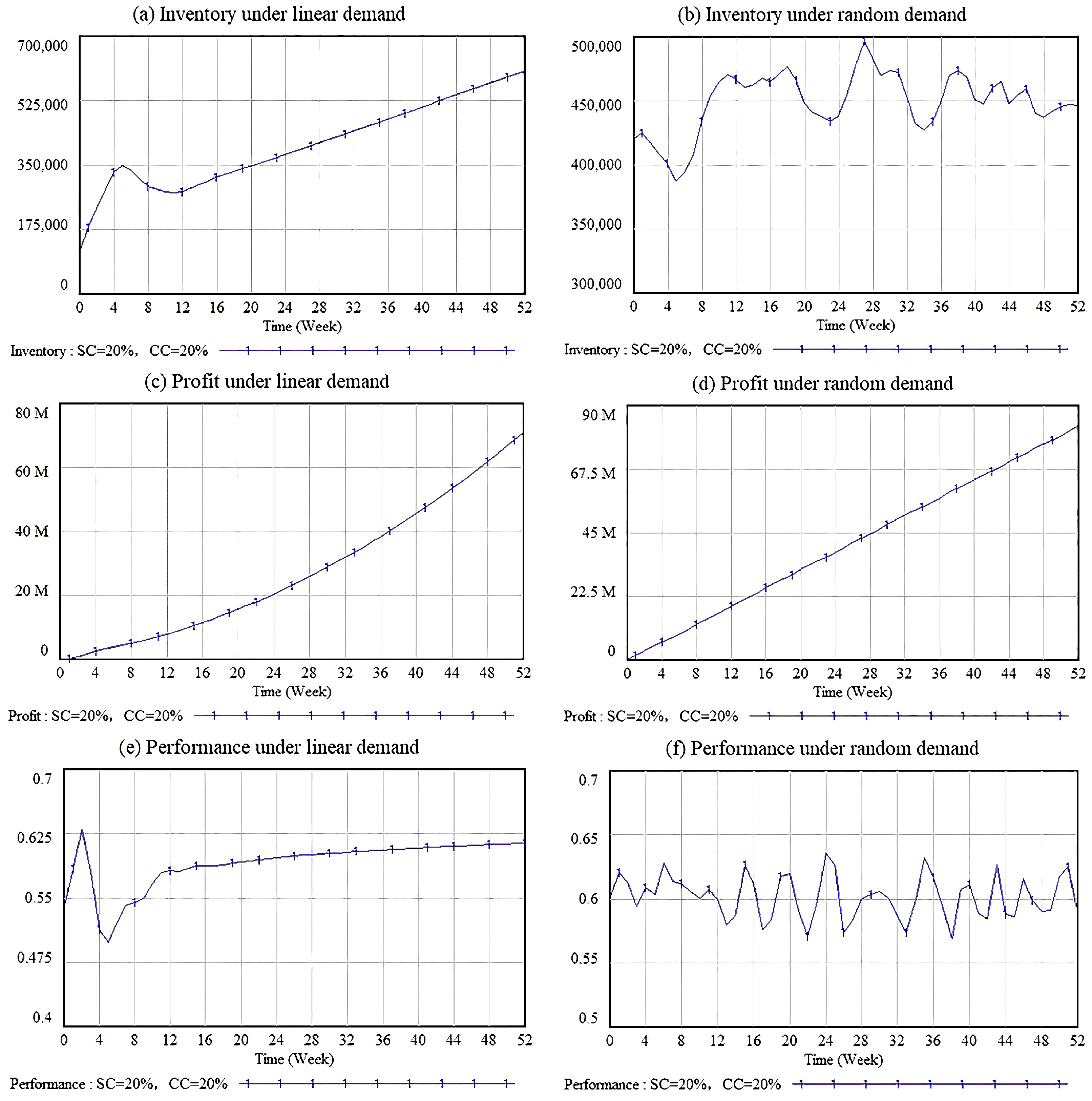
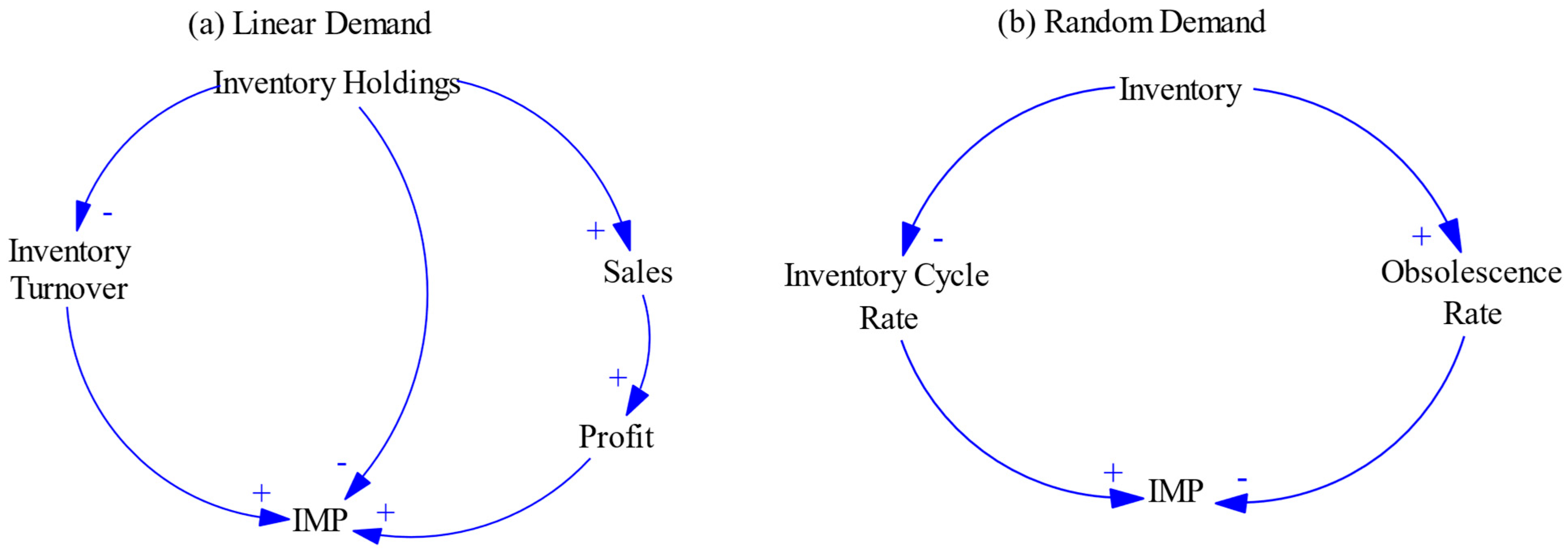
Under the linear growth demand pattern, with all other equations and parameters remaining unchanged, the actual market demand is configured according to Equation (33). Figure 7 presents the simulation results from the SD model, while Figure 8a illustrates the interrelationships among key variables.

Inventory levels increase rapidly in the first 5 weeks, then show slow linear growth after a small drop from Week 5 to Week 12 (Figure 7a). Typically, in manufacturing enterprises, future demand is forecasted based on historical order data, and production is arranged accordingly. In the first five weeks, the initial production is higher than the initial market demand, resulting in increased inventory. Then, inventory levels begin to fall (Weeks 5–12) as subsequent market demand grows rapidly, while forecasts remain low due to low initial demand and insufficient historical demand data. After Week 13, demand forecasts become equal to the actual demand because the demand information is enough to make the demand forecast. There are still some small differences between the forecast and the actual demand, due to the low CC. A low CC indicates dispersed customer demand. The accuracy of the demand forecast decreases, which causes a continuous increase in inventory. This tendency indicates that the interaction between production planning and demand forecasting is that early overproduction is accumulated and the discrepancies are corrected by subsequent adjustments as the forecasts become more accurately adjusted to the actual demand. A low CC enhances the pressure of the demand, decreasing the accuracy of the forecast, and thus leads to long-run inventory levels, and this is in line with the Demand Fragmentation Hypothesis [13].

Profits show a nonlinear increase, with an increasing slope over the simulation period (Figure 7c). In this case, profit means the accumulated profit. If more profit was made, it would mean more money would be available to the company. That is, accumulated profit means the total profit up to that specific moment. When the growing demand of the market was met, periodic profits increased with the sales volume, which drove the continuous increase in cumulative profit. The increase in profit shows that the interaction between operational efficiency gains and inventory management eventually affects the financial outcomes, and thus, the feedback loop between the production, sales and resource allocation in the SD model.

IMP exhibits a rapid upward trend in the first 2 weeks, a shaky upward trend after a sharp decline during Weeks 2–5 and levels off at the end (Figure 7e). IMP is influenced by three subsystems. Among these, the stock-out rate is low and stable during the simulation period, and the performance of the customer service subsystem exhibits little change. Thus, IMP is mainly influenced by changes in inventory and gross margins. In the first two weeks of simulation, initial inventory is low with relatively high inventory turnover and low inventory inactivity rate and IMP increases significantly. During Weeks 2–5, production exceeds the shipment volume, so IMP consequently decreases due to rising inventory and a sharp decrease in inventory turnover. IMP rebounds from Week 5 to Week 12, as inventory decreases and inventory turnover increases. After Week 12, the performance of the inventory and financial subsystems offset each other, due to the faster profit growth rate, resulting in IMP gradually plateauing. Mechanistically, IMP is largely influenced by the coordination between inventory and profit subsystems, which captures the dynamic effects of the SC and CC on supply chain stability and financial performance. A high SC enhances supplier coordination and a low CC leads to forecast uncertainty. These are in line with previous research on power in bargaining and fragmentation in demand [11,13].

5.1.2. Simulation of Basic Scenario Under Random Demand Pattern

Under the random demand pattern, the actual market demand is defined by Equation (34). The market demand for the manufacturing enterprise is simulated under this scenario and the resulting interactions among key variables are depicted in Figure 8b.

Inventory levels initially exhibit considerable fluctuation but gradually stabilize as the simulation progresses (Figure 7b). A notable inflection point emerges later in the simulation, which can be attributed to the inherently unpredictable nature of the random demand pattern.

Profits show a wavy growth trend over the simulation period (Figure 7d), since the weekly product revenue fluctuates with sales, highlighting that financial performance under stochastic conditions is tightly coupled with operational resilience and inventory flexibility.

IMP exhibits a fluctuating trend, with a decreasing fluctuation amplitude as the simulation period progressed (Figure 7f). Different from the linear growth demand model, IMP is mainly affected by inventory, as the changes in gross margin and stock-out rate were not large. The trend of IMP is opposite to that of inventory levels. When inventory levels increase, IMP decreases, due to lower inventory turnover and a higher obsolescence rate; the reverse is also true. Inventory and IMP exhibit higher volatility compared to the linear growth scenario. This demonstrates how demand uncertainty interacts with SCC, where SC mitigates the supply risk, but CC influences the forecast accuracy. Such dynamics align with empirical findings on supply chain risk and concentration effects [6].

The analysis of the linear and random demand conditions demonstrates that the SC and CC affect IMP in different ways. SC mostly influences the supply stability and efficiency in coordination, and CC influences the accuracy of the demand predictions and the manifestation of the bargaining power in the supply chain. In both demand environments, inventory dynamics dominate the cause of the evolution of IMP and, consequently, rely on the accuracy of the forecasts. As the Demand Fragmentation Hypothesis would suggest, a low CC causes dispersed customer demand and, in turn, lowers the forecasting accuracy and, as a result, increases the inventory variability. Based on these observations, the next section modifies the SCC to study how the SC and CC interact to determine the nature of IMP when different patterns of demand are taken.

5.2. Sensitivity Analysis

To examine the effects of the SC and CC on the IMP of manufacturing enterprises, we designed multiple simulation scenarios by adjusting the SC and CC values under both linear and random demand patterns. These scenarios, summarized in

Table 11. Simulation scheme for sensitivity analysis of SC and CC.

Simulation Scenarios	Scheme	SC (%)	CC (%)
Basic Scenario	Base	20	20
Scenarios for Different Levels of SC	A1	30	20
	A2	40	20
	A3	50	20
	A4	60	20
	A5	70	20
Scenarios for Different Levels of CC	B1	20	30
	B2	20	40
	B3	20	50
	B4	20	60
	B5	20	70
Scenarios for Different Levels of SCC	C1	30	20
	C2	20	30

, enable a systematic sensitivity analysis.

Additional tests show that when SC > 80%, inventory volatility exceeds 30%, further supporting the 50% threshold.

5.2.1. Sensitivity Analysis of the Model Under Linear Growth Demand

Under the linear growth demand pattern, market demand is defined by Equation (33). A sensitivity analysis is conducted under this pattern by simulating different scenarios outlined in Table 11.

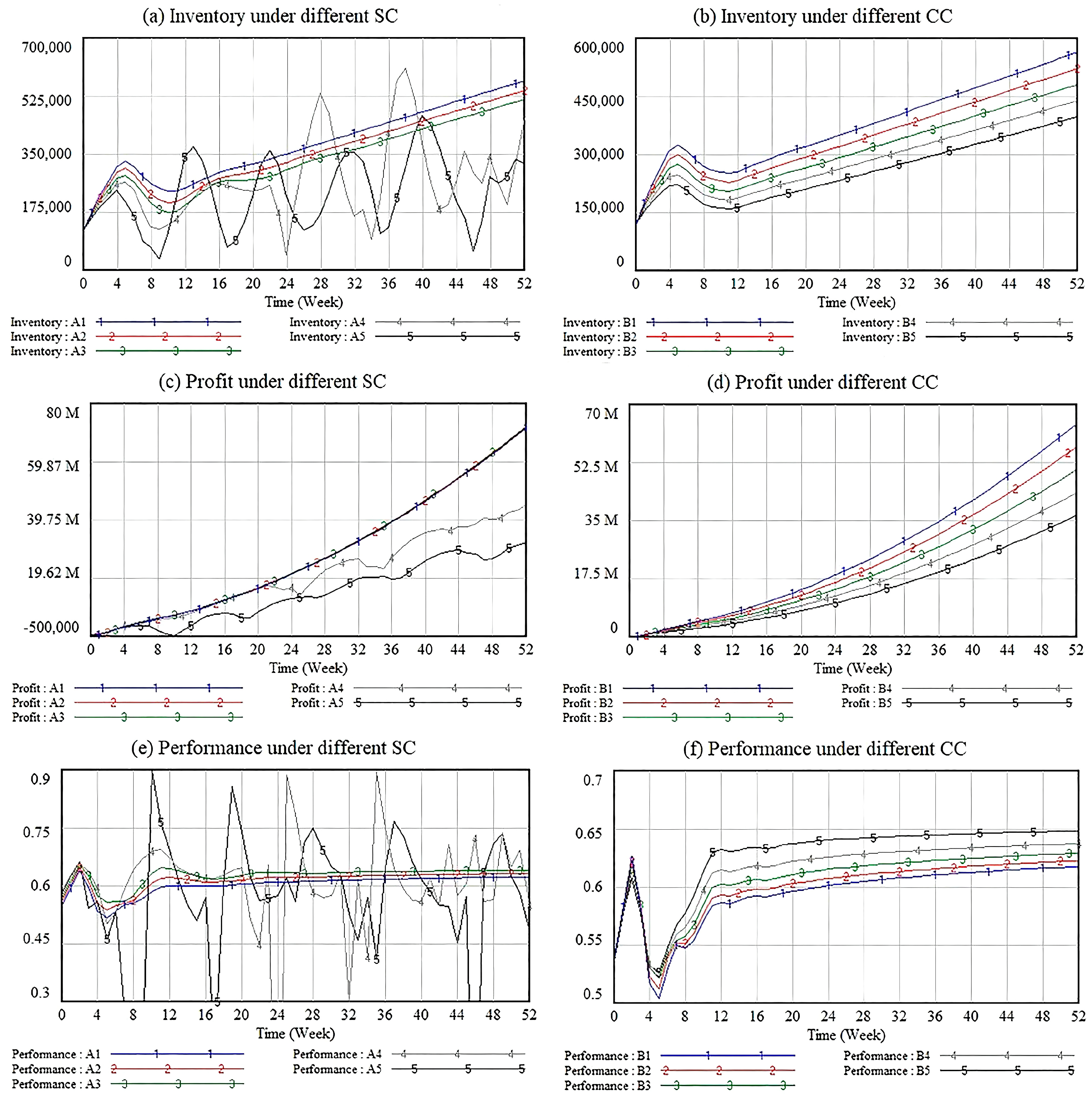
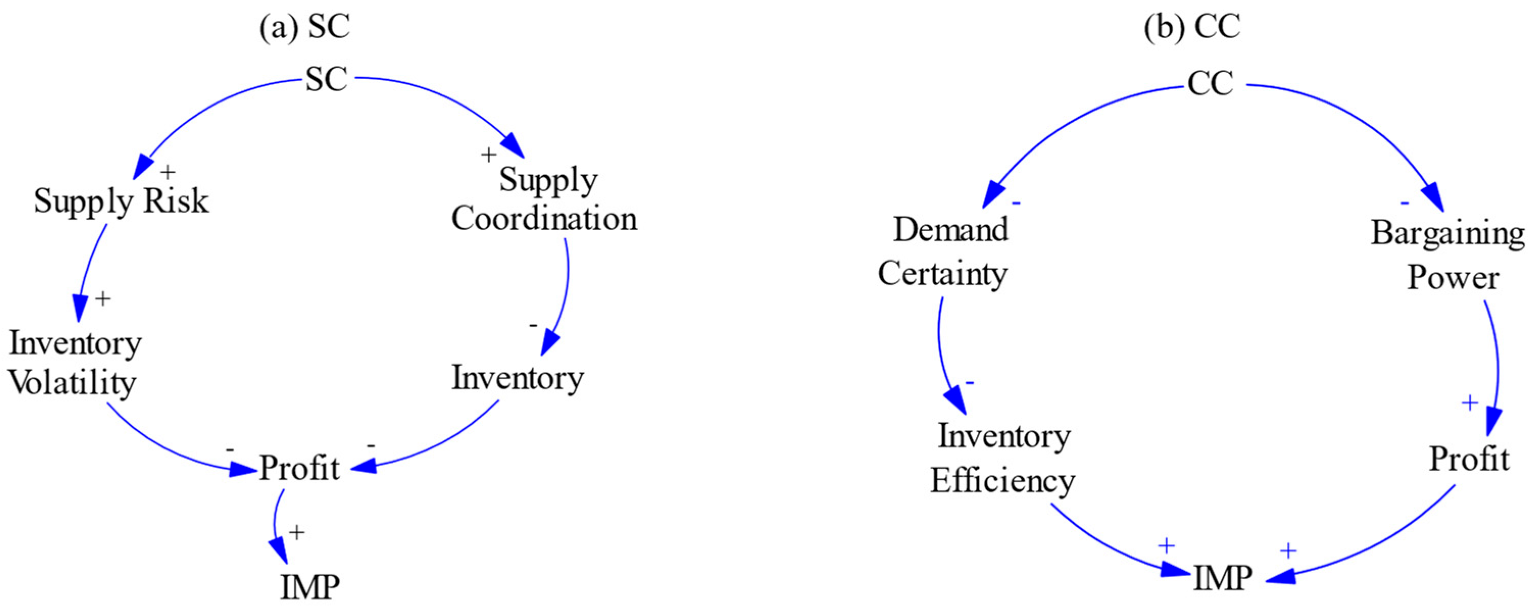
First, we analyze the sensitivity of inventory to different SC levels. Within the 30–50% interval, inventory decreases monotonically with an increasing SC (Figure 9a). Beyond the 50% level, the decreasing trend continues, but with much larger fluctuations: inventory repeatedly achieves close to zero levels (Weeks 9, 35, 46) but also increases substantially above the mean (Weeks 13, 28, 38). This result emerges because higher levels of SC allow for greater procurement concentration and faster material coordination, which systematically decrease inventory. Conversely, when the SC exceeds the threshold of 50%, it results in reduced supply chain redundancy and larger variability in material coordination from the two dominant suppliers, thus explaining the increased inventory fluctuations. Furthermore, we find that the SC has a significant inverted-U relationship with both profit and IMP: within the 30–50% range, both measures increase steadily with SC; beyond 50%, both measures decrease with increasing volatility (Figure 9c,e). The mechanism illustrated in Figure 10a shows that a moderate SC improves supply stability and efficiency; high procurement concentration further concentrates supply risks, which then reduce both profit and IMP.

Next, the influence of the CC is analyzed. The CC shows a significant U-shaped relationship with IMP, while inventory and profit decrease monotonically as CC increases (Figure 9b,d). Specifically, IMP first decreases (Weeks 0–4) and then increases consistently (Weeks 4–52; Figure 9f). The mechanism for this U-shaped effect is depicted in Figure 10b; in the early stage, a low CC confers advantages in bargaining power and profitability, but in the mature stage, a higher CC becomes beneficial, as closer customer relationships reduce demand uncertainty and enhance inventory efficiency.

Finally, the impact of different SCC schemes is examined. Figure 11a shows that the IMP of Scheme C1 is consistently higher than that of Scheme C2 (Table 11). Notably, adjusting the SC yields higher IMP than adjusting the CC, and the improvement magnitude of IMP from SC adjustment gradually diminishes as the enterprise’s operating time progresses, likely due to the gradual stabilization of supply chain operations.

5.2.2. Sensitivity Analysis of the Model Under Random Demand

Under the random demand pattern, the actual market demand is set according to Equation (34). Sensitivity analysis is performed, based on the scenarios defined in Table 11.

First, regarding the impact of different SC levels under a random demand, the simulation results show that the trends of inventory (Figure 12a), profit (Figure 12c) and IMP (Figure 12e) remain consistent with those under the linear growth demand pattern.

Next, regarding the impact of different CC levels under a random demand, the trends of inventory (Figure 12b) and profit (Figure 12d) are also consistent with those under a linear growth demand. As shown in Figure 12f, IMP varies greatly in the first 10 weeks and then increases with an increasing CC. The result indicates that the effect of a high CC on reducing inventory is not robust in the early period: the inventory level under a higher CC is not necessarily smaller than that under a lower CC, which further leads to the trend of IMP. Remarkably, the advantage of a high CC exists more remarkably after volatility. Therefore, the CC should be controlled in a certain range in the early stage to keep IMP at a relatively high level. In the late stage, more attention should be paid to the efficiency of inventory operation, instead of obtaining high and stable profitability. As shown in Figure 12f, fluctuation appears in IMP in the first 10 weeks and then continuously increases with the increase in CC. This means that the effectiveness of a high CC for reducing inventory is not very sensitive in the early operation stage: the IMP is not necessarily lower than that in the lower CC group for the early stage of the CC increasing; namely, the IMP is not always lower in the higher CC group than that in the lower CC group, and then the IMP presents the above fluctuation. Importantly, the relative advantage of a high CC appears after the early stage: namely, the CC should be controlled in the moderate range during the early stage, and then IMP can be kept at relatively high level. During the later stage, more attention should be paid to the efficiency of inventory.

Finally, regarding the impact of different SCC schemes, the results show that the IMP of Scheme C1 is slightly higher than that of Scheme C2. Additionally, higher IMP can be achieved by adjusting the SC rather than the CC. However, the efficiency of SC adjustment in improving IMP under a random demand is demonstrated to be lower than that under a linear growth demand (Figure 11b).

Overall, the sensitivity analysis implies that the SC and CC influence inventory behaviors, profit behavior and IMP, with the help of various pathways that differ according to demand patterns. The SC can be linked to supply stability and coordination efficiency, whereas the CC affects the accuracy of demand forecasts, with forecasts and inventory decisions varying accordingly. The analysis also defines obvious nonlinear features such as the threshold effects of SC and the U-shaped effects of CC. These trends assert the way inventory performance dynamically evolved through a modification in the design of suppliers and customers. Moderate levels of the SC enhance coordination and decrease the variability of the inventory, yet extreme high levels of the SC form a more susceptible system to the issues in the supply. This observation concurs with theoretical insights, as provided by the resource dependence theory, and the overall OM body of literature [8,11,13]. Combined, the findings conceptually justify the argument that changing supplier and customer relationships constitute an efficient strategy towards ameliorating supply chain organization when operating in a dynamic market environment.

6. Conclusions and Future Work

6.1. Main Results Summary and Implications

This study develops an SD model to examine how the SCC influences IMP in manufacturing enterprises under different demand environments. By constructing dynamic feedback loops and simulating linear and random demand scenarios, the analysis identifies nonlinear and threshold-based effects that static cross-sectional approaches cannot reveal. The results directly respond to the research questions by offering three key insights. First, the SD framework captures the evolving interaction between the SCC and IMP, highlighting its nonlinear feedback structure. Second, contrasting the two demand scenarios shows that the SCC does not exert uniform effects across environments, as both the SC and the CC vary in magnitude and direction with rising demand uncertainty. Third, incorporating enterprise lifecycle stages clarifies why the SCC affects IMP differently in early versus mature phases, providing a mechanism-based explanation for the heterogeneous impacts. These mechanisms jointly demonstrate that the conclusions of the study arise directly from the simulation outputs and are consistent with the established findings in the literature. The key conclusions are as follows:

(1) Under both linear growth and random demand patterns, the impact of the SC on IMP for manufacturing enterprises consistently exhibits an inverted U-shaped relationship. An optimal equilibrium point exists at SC = 50%, with a moderate interval of 30% to 50%. Before this equilibrium point, IMP increases with the rise in SC, which helps enterprises coordinate with core suppliers for raw material supply and decreases the finished goods inventory level. However, after this equilibrium point, the increase in the SC leads to a decrease in IMP. This decline occurs because higher SC increases supply chain dependence. When delays arise among concentrated suppliers, enterprises face difficulties with meeting customer demand and maintaining stable inventory control, ultimately reducing IMP. These results are directly supported by the model simulation outputs, confirming the theoretical expectation that excessive concentration raises vulnerability. This explanation contributes to a balanced discussion of both the positive and negative effects associated with SC.

(2) When demand grows in a linear form, the CC and IMP present a U-shaped relationship in the long run; when the demand is random, IMP will fluctuate when the CC exceeds 50% in the first ten weeks and then has a continuously positive effect afterwards. Therefore, when the CC enhances IMP in practice, the time-separation should be presented. The enterprise whose demand grows linearly should decrease the CC in the initial stage to enhance the bargaining power of the downstream; the enterprise whose demand is random should control the CC below 50% initially, to reduce fluctuation, and then increase the CC in a later stage to gain demand consolidation without a service-level decrease. These findings suggest that CC management should differentiate between demand types, with staged adjustment strategies applied to balance stability and bargaining power.

(3) Under either a linear growth or random demand, the SC has a more significant effect on IMP than the CC. Raw material procurement and supplier management should be prioritized for manufacturers to improve IMP. This conclusion is consistent with both the simulation evidence and the consensus view in the supply chain management literature, further supporting its robustness.

Based on the research conclusions, we provide practical directions for manufacturing listed enterprises to optimize IMP. Enterprises should establish a dynamic SC control mechanism, centered on the “top five procurement proportions,” and regularly review this ratio, deepen cooperation with core suppliers when it is low, reserve alternative suppliers when it is high and maintain it within the range of 30% to 50% to balance efficiency and risk. CC management should align with the “demand model and enterprise stage” framework: under a linear growth demand, newly established enterprises should focus on customer diversification to enhance bargaining power, while mature enterprises may moderately increase the CC to strengthen demand synergy. When the demand is randomly presented, the enterprise is suggested to firstly control the proportion of the top five buyers and then gradually advance the adjustment of the rest. Resource allocation should first prioritize procurement optimization and supplier structure design. On this basis, the real-time tracking system of the top five procurement and sales proportions should be established, with the early warning value specified in advance. It is expected that the SC and CC can be converted from static indicators into dynamic management tools, and the inventory efficiency and chain reliability will be improved accordingly.

6.2. Future Research

This study, in comparison to the existing literature, contributes to the literature because it shows that there is a nonlinear dynamic relationship between the SC and CC and IMP. Past empirical studies primarily use cross-sectional or panel-data designs and tend to indicate varied linear impacts of the SCC on operational results [11,17]. Such approaches often treat concentration indicators as fixed attributes, overlooking the evolving system-level interactions. Conversely, this paper uses a system dynamics model to indicate the internal feedback between the concentration and inventory performance. The findings indicate that the impacts of the supplier and the CC are different in varying demand environments and levels of the lifecycle of an enterprise, which gives a mechanism-based explanation of why the current research has largely heterogeneous results.

Irrespective of these contributions, there are several limitations which should be taken into consideration. Only using two patterns of demand used in the analysis, linear growth and random demand, does not allow for representing more complex market changes like seasonal, cyclical or promotion-driven changes [27]. The research is limited to manufacturing organizations, and the supply chain in the retail, service or digital platform sectors may have quite different designs [33]. Moreover, the models of the supplier and the CC are reduced to a simplistic level and do not reflect the heterogeneity, multi-tier relationships and different behavioral features of the real supply networks. Such simplifications can make the findings less applicable to more industrial-based situations.

These shortcomings offer some possible directions for further studies. Another potential area of extension is to include more demand patterns to check the strength of the nonlinear effects found in this study. The second direction is to use the model to test the relationship between the SCC and inventory performance on another industry to determine the influence of sector-specific factors. The next generation of work can be the introduction of additional empirical parameters, multi-level supply chain architecture or decision rules, which will enhance the realism and practical applicability of a model. Additionally, the mathematical modeling of systems with empirical studies like econometric analysis, case-based calibration or data-driven parameter optimization would help in enhancing the empirical base of the research and extending the theoretical contributions to the studies of SCC and IMP.

References

1. Ameh, B. Advancing national security and economic prosperity through resilient and technology driven supply chains. World J. Adv. Res. Rev. 2024, 24, 483–500. [Google Scholar] [CrossRef]
2. Tăbîrcă, A.I.; Radu, V.; Cozorici, A.N.; Tanase, L.C.; Radu, F. Professional Determinants in ESG Reporting for Sustainable Financial Assessment. Systems 2025, 13, 898. [Google Scholar] [CrossRef]
3. UNCTAD. Review of Maritime Transport 2023: Towards a Green and Just Transition; United Nations: Geneva, Switzerland, 2023; Available online: https://unctad.org/rmt2023 (accessed on 14 December 2024).
4. ECB. Geopolitical Fragmentation and Its Impact on Global Trade and Supply Chains. ECB Econ. Bull. 2023, 7, 2839. Available online: https://www.ecb.europa.eu/press/economic-bulletin/html/eb202307.en.html (accessed on 14 December 2024).
5. Ahmadini, A.A.H.; Modibbo, U.M.; Shaikh, A.A. Multi-objective optimization modelling of sustainable green supply chain in inventory and production management. Alex. Eng. J. 2021, 60, 5129–5146. [Google Scholar] [CrossRef]
6. Çömez-Dolgan, N.; Moussawi-Haidar, L.; Jaber, M.Y. A buyer-vendor system with untimely delivery costs: Traditional coordination vs. VMI with consignment stock. Comput. Ind. Eng. 2021, 154, 107009. [Google Scholar] [CrossRef]
7. Maly, L.O.; Avinadav, T. Smart allocation of a developer’s spending on product quality and non-salary employee benefits in a supply chain of apps. Oper. Res. Perspect. 2023, 10, 100261. [Google Scholar] [CrossRef]
8. Hofer, C.; Jin, H.; Swanson, R.D.; Waller, M.A.; Williams, B.D. The impact of key retail accounts on supplier performance: A collaborative perspective of resource dependency theory. J. Retail. 2012, 88, 412–420. [Google Scholar] [CrossRef]
9. Zhu, X.; Zhao Jeihoonian, M.; Kazemi Zanjani, M.; Gendreau, M. Dynamic reverse supply chain network design under uncertainty: Mathematical modeling and solution algorithm. Int. Trans. Oper. Res. 2020, 29, 3161–3189. [Google Scholar] [CrossRef]
10. Wang, J.; Zhang, Y.; Yao, X.; Zhu, X. Lean inventory and ESG performance: An inverted U-shaped relationship. J. Manuf. Technol. Manag. 2025, 36, 123–145. [Google Scholar] [CrossRef]
11. Casalin, F.; Pang, G.; Maioli, S.; Cao, T. Inventories and the concentration of suppliers and customers: Evidence from the Chinese manufacturing sector. Int. J. Prod. Econ. 2017, 193, 148–159. [Google Scholar] [CrossRef]
12. Ak, B.K.; Patatoukas, P.N. Customer-base concentration and inventory efficiencies: Evidence from the manufacturing sector. Prod. Oper. Manag. 2016, 25, 258–272. [Google Scholar] [CrossRef]
13. Olivares, M.; Cachon, G.P. Drivers of finished-goods inventory in the U.S. automobile industry. Manag. Sci. 2010, 56, 202–216. [Google Scholar] [CrossRef]
14. Lanier, D.; Wempe, W.F.; Zacharia, Z.G. Concentrated supply chain membership and financial performance: Chain- and firm-level perspectives. J. Oper. Manag. 2009, 28, 1–16. [Google Scholar] [CrossRef]
15. CATL. Study on the Profit Model of Power Battery Enterprises: CATL’s Customer Concentration Analysis; Report; CATL: Ningde, China, 2021; Available online: https://www.catl.com/static/upload/file/20220421/2021AnnualReport.pdf (accessed on 6 April 2025).
16. Johnson, W.C.; Kang, J.K.; Yi, S. The certification role of large customers in the new issues market. Financ. Manag. 2020, 39, 1425–1474. [Google Scholar] [CrossRef]
17. Patatoukas, P.N. Customer-base concentration: Implications for firm performance and capital markets. Account. Rev. 2012, 87, 363–392. [Google Scholar] [CrossRef]
18. Zhang, X.; Zou, M.; Liu, W.; Zhang, Y. Does a firm’s supplier concentration affect its cash holding? Econ. Model. 2020, 90, 527–535. [Google Scholar] [CrossRef]
19. Pan, J.; Yu, M.; Liu, J.; Fan, R. Customer concentration and corporate innovation: Evidence from China. N. Am. J. Econ. Financ. 2020, 54, 101281. [Google Scholar] [CrossRef]
20. Ren, Y.; Li, J.J.; Zhao, W.; Zhang, L. The delicate equilibrium: Unveiling the curvilinear nexus between supply concentration and organizational resilience. Br. J. Manag. 2024, 35, 1234–1250. [Google Scholar] [CrossRef]
21. Teerasoponpong, S.; Sopadang, A. Decision support system for adaptive sourcing and inventory management in small and medium-sized enterprises. Robot. Comput. Integr. Manuf. 2022, 73, 102226. [Google Scholar] [CrossRef]
22. Kim, D.Y.; Zhu, P.C.; Xiao, W.L.; Lin, Y.-T. Centrality and supplier performance: The moderate role of resource dependence. Oper. Manag. Res. 2021, 14, 22–38. [Google Scholar] [CrossRef]
23. Braglia, M.; Frosolini, M.; Gallo, M. SMED enhanced with 5-whys analysis to improve setup-reduction programs: The SWAN approach. Int. J. Adv. Manuf. Technol. 2016, 90, 1845–1855. [Google Scholar] [CrossRef]
24. Wang, Q.; Peng, Y.; Yang, Y. Solving inventory management problems through deep reinforcement learning. J. Syst. Sci. Syst. Eng. 2022, 31, 677–689. [Google Scholar] [CrossRef]
25. Lu, C.; Ye, Y.; Shi, Z. Optimization of Semi-Finished Inventory Management in Process Manufacturing: A Multi-Period Delayed Production Model. Systems 2025, 13, 879. [Google Scholar] [CrossRef]
26. Kim, S.; Na, J.; Kim, B. Strategic effects of supply chain inventories on sales performance. Eng. Manag. J. 2020, 32, 187–200. [Google Scholar] [CrossRef]
27. Akcay, A.; Corlu, C.G. Simulation of inventory systems with unknown input models: A data-driven approach. Int. J. Prod. Res. 2017, 55, 5826–5840. [Google Scholar] [CrossRef]
28. Qiu, R.Z.; Zhang, D.Q.; Sun, Y.M.; Guan, Z.M. A CVaR-based robust optimization model for retailers’ inventory under supply and demand uncertainty. Chin. J. Manag. Sci. 2020, 12, 98–107. [Google Scholar] [CrossRef]
29. Zhang, W.; Tao, Q.; Feng, Q.; Sun, Y. Supplier concentration and firm risk-taking: Transaction cost perspective. J. Financ. Res. 2024, 133, 106662. [Google Scholar] [CrossRef]
30. Barbrook-Johnson, P.; Penn, A.S. System Dynamics. In Systems Mapping; Springer Nature: Berlin/Heidelberg, Germany, 2022; pp. 113–128. [Google Scholar] [CrossRef]
31. Wu, J.Z.; Zhang, Q.A. Multicriteria decision making method based on intuitionistic fuzzy weighted entropy. Expert Syst. Appl. 2011, 38, 916–922. [Google Scholar] [CrossRef]
32. Li, W.; Chen, J. Manufacturer’s vertical integration strategies in a three-tier supply chain. Transp. Res. Part E Logist. Transp. Rev. 2020, 135, 101884. [Google Scholar] [CrossRef]
33. Wang, Y.; Jia, F.; Schoenherr, T.; Gong, Y.; Chen, L. Cross-border e-commerce firms as supply chain integrators: The management of three flows. Ind. Mark. Manag. 2020, 89, 72–88. [Google Scholar] [CrossRef]
34. Chen, M.; Tang, X.; Liu, H.; Gu, J. The impact of supply chain concentration on integration and business performance. Int. J. Prod. Econ. 2023, 257, 108781. [Google Scholar] [CrossRef]
35. Deng, S.; Xu, J.; Han, Y. A proprietary component manufacturer’s global supply chain design: The impacts of tax and organizational structure. Omega 2023, 115, 102777. [Google Scholar] [CrossRef]
36. Yli-Renko, H.; Denoo, L.; Janakiraman, R. A knowledge-based view of managing dependence on a key customer: Survival and growth outcomes for young firms. J. Bus. Ventur. 2020, 35, 106045. [Google Scholar] [CrossRef]
37. Li, Y.; Wang, H. Synchronized production and maintenance scheduling for turnover reliability. J. Manuf. Syst. 2022, 62, 726–736. [Google Scholar] [CrossRef]
38. Reddy, K.J.M.; Rao, A.N.; Krishnanand, L. Manufacturer performance modelling using system dynamics approach. Mater. Today Proc. 2020, 33, 142–146. [Google Scholar] [CrossRef]
39. Derwik, P.; Hellström, D. Successful competence development for retail professionals: Investigation of key mechanisms in informal learning. Int. J. Retail Distrib. Manag. 2023, 51, 33–46. [Google Scholar] [CrossRef]
40. Tencent News. Reasons for the Price Increase of Storage IC Chips and the Latest Market Forecast. Tencent News. 12 October 2023. Available online: https://news.qq.com/rain/a/20231012A07C5O00 (accessed on 11 August 2025).
41. Womack, J.P.; Jones, D.T. Lean Thinking: Banish Waste and Create Wealth in Your Corporation; Simon & Schuster: New York, NY, USA, 1996. [Google Scholar]
42. Siemens AG. Digital Enterprise Case Study: Amberg Plant; Siemens AG: Munich, Germany, 2023; Available online: https://techorange.com/2023/04/19/siemens-amberg/ (accessed on 11 August 2025).
43. Inditex Group. Annual Report 2023; Inditex: Arteixo, Spain, 2023; Available online: https://static.inditex.com/annual_report_2023/en/Inditex_Group_Annual_Accounts_2023.pdf (accessed on 11 August 2025).
44. Dell Technologies. Supply Chain Sustainability Report; Dell Technologies: Round Rock, TX, USA, 2022; Available online: https://www.delltechnologies.com/asset/de-at/solutions/business-solutions/briefs-summaries/delltechnologies-fy23-supply-chain-sustainability-summary.pdf (accessed on 11 August 2025).
45. Tencent Cloud. How P&G Uses EDI to Achieve Supply-Chain Integration. Tencent Developer Community. 18 August 2021. Available online: https://cloud.tencent.com/developer/article/1864228 (accessed on 11 August 2025).
46. Aljuhmani, A.I.; Alomari, M.A. Inventory Turnover and Firm Profitability: A Saudi Arabian Manufacturing Sector Perspective. Processes 2023, 11, 716. [Google Scholar] [CrossRef]
47. Anderson, E.W.; Fornell, C.; Lehmann, D. Customer satisfaction, market share, and profitability: Findings from Sweden. J. Mark. 1994, 58, 53–66. [Google Scholar] [CrossRef]
48. SiTime Corporation. Annual Report 2022; SiTime Corporation: Santa Clara, CA, USA, 2022; Available online: https://www.sgpjbg.com/baogao/564042.html (accessed on 11 August 2025).
49. Shanghui Certified Public Accountants (Special General Partnership). Reply to the Second Round of Review Inquiries Regarding the Initial Public Offering and Listing on the Growth Enterprise Market of Shandong SanYuan Biotechnology Co., Ltd. (Updated with 2021 Semi-Annual Report Data); Sina Finance: Beijing, China, 2021; Available online: https://vip.stock.finance.sina.com.cn/corp/view/vCB_AllBulletinDetail.php?id=7575845 (accessed on 11 August 2025).
50. Fonseca, L.; José Carlos, S.Á.; Lima, V. Evaluating the synergy between lean practices and sustainability in supply chains: A conceptual framework for supplier assessment. Sustain. Dev. 2025, 33, 1–18. [Google Scholar] [CrossRef]
51. Davizón, Y.A.; Hernández-Santos, C.; de la Cruz, N.; Garcia-Andrade, R.; Ramirez, A.F.; Hernández, A.; Tobías-Macías, F.F.; Rincón, E.; Reyes, A.-M.; Smith, E.D. Mathematical Methods for Inventory Management in Dynamic Supply Chains. Systems 2025, 13, 920. [Google Scholar] [CrossRef]
Figure 1. Comprehensive sensitivity analysis of IMP weights in SCC, based on Table 1.
Systems 13 01084 g001
Figure 2. SD model of the interaction between SCC and IMP via multi-flow coordination and bilateral feedback mechanisms.
Systems 13 01084 g002
Figure 3. Causal loop diagram of SCC and IMP with eight feedback paths.
Systems 13 01084 g003
Figure 4. Stock and flow diagram of SCC and IMP with eight feedback paths.
Systems 13 01084 g004aSystems 13 01084 g004b
Figure 5. Three-dimensional surface plots of simulated and actual IMP, varying with SC and CC.
Systems 13 01084 g005
Figure 6. Comparison of actual and simulated IMP with linear fitting for TIANCI and SOGAL.
Systems 13 01084 g006
Figure 7. SD simulation results for inventory, profit and IMP under different demand patterns.
Systems 13 01084 g007
Figure 8. Causal loop diagrams of inventory, profit and IMP under different demand patterns.
Systems 13 01084 g008
Figure 9. Sensitivity analysis of inventory, profit and IMP under linear growth demand pattern.
Systems 13 01084 g009
Figure 10. Causal loop diagrams for SC and CC’s impact on inventory and profit, with IMP.
Systems 13 01084 g010
Figure 11. Sensitivity analysis of IMP with different SCC, under different demand patterns.
Systems 13 01084 g011
Figure 12. Sensitivity analysis of inventory, profit and IMP under random demand pattern.
Systems 13 01084 g012