Predicting Protein–Protein Interactions Based on Ensemble Learning-Based Model from Protein Sequence

Simple Summary

Due to most traditional high-throughput experiments are tedious and laborious in identifying potential protein–protein interaction. To better improve accuracy prediction in protein–protein interactions. We proposed a novel computational method that can identify unknown protein–protein interaction efficiently and hope this method can provide a helpful idea and tool for proteomics research.

Abstract

Protein–protein interactions (PPIs) play an essential role in many biological cellular functions. However, it is still tedious and time-consuming to identify protein–protein interactions through traditional experimental methods. For this reason, it is imperative and necessary to develop a computational method for predicting PPIs efficiently. This paper explores a novel computational method for detecting PPIs from protein sequence, the approach which mainly adopts the feature extraction method: Locality Preserving Projections (LPP) and classifier: Rotation Forest (RF). Specifically, we first employ the Position Specific Scoring Matrix (PSSM), which can remain evolutionary information of biological for representing protein sequence efficiently. Then, the LPP descriptor is applied to extract feature vectors from PSSM. The feature vectors are fed into the RF to obtain the final results. The proposed method is applied to two datasets: Yeast and H. pylori, and obtained an average accuracy of 92.81% and 92.56%, respectively. We also compare it with K nearest neighbors (KNN) and support vector machine (SVM) to better evaluate the performance of the proposed method. In summary, all experimental results indicate that the proposed approach is stable and robust for predicting PPIs and promising to be a useful tool for proteomics research.

1. Introduction

Protein–protein interactions (PPIs) play a crucial role in almost all cellular processes and functions, such as DNA transcription and replication, immune response, signal transduction, and gene expression [1,2]. Thus, detecting and characterizing potential protein interactions correctly are significant for understanding the properties of biological processes. Recently, a number of innovative high-throughput biological experimental technologies, including yeast two-hybrid screen (Y2H) [3,4], protein chip [5], and tandem affinity purification tagging (TAP) [6], and other methods have been proposed to detect the interaction between proteins systematically. With the development of biotechnology, the number of PPI data is quickly accumulating. For this reason, multiple databases have been built to record PPI data efficiently. Biomolecular Interaction Network Database (BIND) [7], Database of Interacting Proteins (DIP) [8], and the Molecular Interaction database (MINT) [9] are mainly used databases by researchers. However, there still exist some drawbacks to traditional high-throughput methods, such as being costly and labor-intensive and it will raise a high rate of false positives. The known PPI pairs which have been validated through biological experiment methods only account for a small portion of the whole PPI network [10,11]. As a result, developing a novel computational method is conducive to inferring potential PPIs.

Up to now, a great number of computational techniques have been proposed for predicting potential PPIs [12,13,14]. Generally, some existing methods for predicting PPIs typically can be treated as binary classification problems which adopt different features to represent protein pairs [15,16,17]. Different feature sources or protein attributes like protein domains, phylogenetic profiles, and protein structure information are employed to detect potential protein interactions. There are also exist methods that utilize interaction information from several different protein features [18,19]. However, these approaches are not easy to implement unless pre-knowledge of protein pairs can be available.

Recently, a couple of computational methods mainly based on protein sequences have been proposed since protein sequences are the easiest to obtain [20,21,22]. Many researchers have engaged in the development of a sequence-based method for detecting potential PPIs [23,24,25,26], and a variety of experimental results indicated that it is sufficient to predict PPI using the information of amino acid sequences alone [27,28,29,30,31]. For instance, Xia et al. [32] proposed that the Moran autocorrelation descriptor can effectively depict the level of the correlation between two protein sequences of specific physicochemical property and use rotation forest to predict PPIs. Shen et al. [33] proposed a computational method that extracts features by utilizing the conjoint triad (CT) which considered the local environments of residues, and then using a support vector machine (SVM) to predict PPIs; this method achieved the result of average accuracy of 83.9%. You et al. [34] developed a novel computational method that used multi-scale continuous and discontinuous (MCD) to represent protein sequence and achieved an excellent result in the Yeast dataset. Chen et al. [35] reported an approach that uses XGBoost to reduce feature noise and adopts StackPPI that several ensemble classifiers to detect the interaction of protein pairs. Zhao et al. [36] proposed an ensemble method and the results of the proposed method obtained good performance. Yousef et al. [37] developed a sequence-based, fast, and adaptive PPIs prediction method, which employed principal component analysis (PCA) as a proper feature extraction method and utilized adaptive learning vector quantization (LVQ) to predict different PPI datasets. This method achieved an average accuracy of 93.88% and 90.03% on S. cerevisiae and H. pylori, respectively. Wang et al. [38] reported an approach only using the information of protein sequence; the approach combined continuous and discrete wavelet transforms and weight sparse representation-based classifier for predicting PPIs. Zahiri et al. [39] proposed a novel evolutionary-based algorithm called PPIevo, which extracts features from PSSM for predicting protein–protein interactions. In general, previous works illustrate that the feature extraction method and classification are the two most important steps to predicting PPIs.

In this paper, by fully using evolutionary information of protein sequence, we report a novel computational method, which obtaining numerical representation by Position Specific Scoring Matrix (PSSM), extracting feature vector by using locality preserving projections (LPP), and predicting by rotation forest (RF) classifier. More Specifically, the first step is transforming protein sequence into numerical representation, PSSM. Second, each PSSM can be extracted by LPP, and obtained a low-dimensional feature vector. Finally, the feature descriptors are fed into the RF classifier for inferring potential protein–protein interactions. Two datasets, Yeast and H. pylori, are applied in our proposed method; the five-fold cross-validation results of average accuracy are 92.81% and 92.56%, respectively. The performance of our proposed approach is better than the support vector machine (SVM), K nearest neighbors. We also performed extensive experiments on four cross-species independent datasets. Experimental results show that the proposed method outperforms other existing methods and we hope this approach can provide a solution for inferring potential PPIs.

2. Materials and Methods

2.1. Datasets

The dataset can help us know whether the performance of the proposed method is good or not. In this study, we adopt two benchmark datasets to evaluate the model. Firstly, from the DIP database [8], the Yeast PPI dataset was collected. For enhancing credibility, the length of protein pairs that were less than 50 residues and protein pairs that have more than forty percent sequence identity will be directly removed. Thus, the Yeast dataset was constructed by 11,888 protein pairs, including a positive dataset of 5594 protein pairs and a negative dataset of 5594 protein pairs. The second dataset—the H. pylori PPI dataset—is described by Martin et al. [40]; the whole dataset is constructed by 2916 protein pairs (1458 interacting pairs and 1458 non-interacting pairs).

2.2. Position Specific Scoring Matrix

Position-Specific Scoring Matrix (PSSM) [41] is widely used for transform biological sequence into numerical representation [42,43]. Given a protein sequence with length N, The PSSM can be represented as follows:

$$D=\left[\begin{array}{cccc}{\alpha }_{1,1}& {\alpha }_{1,2}& \cdots & {\alpha }_{1,20}\\ {\alpha }_{2,1}& {\alpha }_{2,2}& \cdots & {\alpha }_{2,20}\\ ⋮& ⋮& \ddots & ⋮\\ {\alpha }_{N,1}& {\alpha }_{N,2}& \cdots & {\alpha }_{N,20}\end{array}\right]$$

(1)

where ${\alpha }_{i,j}$ means the probability of the ith residue being mutated into type j of 20 native amino acids during the evolutionary process of the protein from multiple sequence alignments. In this step, employing the tool mentioned in [44] can convert each protein sequence into PSSM.

2.3. Locality Preserving Projections

We aim to extract the feature vectors, which mainly reduce the dimensional of the original matrix to reduce the influence of noise. In this section, Locality Preserving Projections (LPP) algorithm [45] is adopted for extracting feature vectors in each PSSM. It adopts a linear approximation to the Laplace characteristic map for obtaining the structure feature between neighboring. Thus, it is widely used for data processing and analysis application. Given a training sample $X={\left[x_1,x_2,\dots ,x_n\right]}^T\in R^D$, where D is the feature dimension, and n denotes the feature vectors of each sample. Then for projecting the high-dimensional input dataset X into a low-dimensional dataset $Y=\left[y_1,y_2,\dots ,y_n\right]$, it is necessary to seek a projection matrix W. The objective function of LPP is defined as

$$argmin{\displaystyle \sum }_{i,j=1}^m{\left(y_i-y_j\right)}^2{P}_{ij}$$

(2)

where

$$P_{ij}=\{\begin{array}{c}\exp \left(-\frac{{\Vert x_i-x_j\Vert }^2}{t}\right), x_i and x_j is linked \\ 0, x_i and x_j is not linked \end{array}$$

(3)

$$y_i=w^T{x}_i$$

(4)

where $P_{ij}$ is the heat kernel, w denotes a transformation vector, and in Equation (3), the parameter t means scale size. Thus, we can define the distance formula is shown as follows:

$$d(x_i,x_j)=\Vert x_i-x_j\Vert$$

(5)

Then, it is necessary to minimize the projection matrix W. The steps are defined as:

$$\begin{array}{c}\frac{1}{2}{\displaystyle \sum _{i,j}}{\left(y_i-y_j\right)}^2{P}_{ij}=\frac{1}{2}{\displaystyle \sum _{i,j}}{\left(w^T{x}_i-w^T{x}_j\right)}^2{P}_{ij}\\ =w^{T}X\left(D-W\right)X^{T}w=w^{T}XL{X}^{T}w\end{array}$$

(6)

where D is a diagonal matrix, $Dii={{\displaystyle \sum }}_{j=1}^n{W}_{ij}$ and $L=D-W$ represent the Laplacian matrix. The constraint is:

$$w^{T}XD{X}^{T}w=1$$

(7)

Finding a transfer matrix w, the following generalized eigenvalue problem:

$$XL{X}^{T}w=\lambda XD{X}^{T}w$$

(8)

Solving the question in Equation (8), we can obtain all the eigenvalues and eigenvectors corresponding, k eigenvalues: ${\lambda }_0,{\lambda }_1,\dots ,{\lambda }_{k-1}$ are sorted from small to large. $\{w_0,w_1,\dots ,w_{k-1}\}$ denotes the corresponding characteristic vectors. First, l eigenvectors are selected to form the projection matrix $W=[w_0,w_1,\dots ,w_{l-1}]$. As a result, the embedding descriptors are

$$x_i\to y_i=W^T{x}_i$$

(9)

2.4. Rotation Forest

Rodriguez et al. [46] proposed rotation forest (RF) is a typical ensemble learning algorithm that is widely used in the classification task. In the RF algorithm, it first divides the feature set into K subsets by randomly combining the features of the sample. Principal component analysis (PCA) is then used to transform the data and retain the accuracy of the original data. As a result, RF improves classification performance by amplifying the differences between base classifiers.

Let training sample set S be an $M\times m$ matrix. m represents the feature vector length of each training sample. Let X be the feature set, and $Y={\left(y_1,y_2,\dots ,y_n\right)}^T$ are corresponding labels. Assuming L decision tree, which can be denoted as $[Q_1,Q_2,\dots ,Q_L]$, respectively. In this algorithm, the complete feature set will be divided into K subsets equally and randomly. A single classifier $Q_i$ of processing steps can be summarized as follows:

(1)

Set X is randomly divided into K disjoint subsets; each subset contains the number of features is $C=M/K$.

(2)

Form a new matrix $S_{i,j}$ by choosing the corresponding column of the feature in the subset $Q_{i,j}$ from the training dataset S. And applying a bootstrap sampling technique from seventy-five percent of the original training dataset S to generate a new matrix $S_{j,j}^{\prime }$.

(3)

Employ C feature by adopting the PCA method in matrix $S_{j,j}^{\prime }$. The principal component coefficients are stored in $T_{i,j}$, which can be represented as ${\gamma }_{ij}^{\left(1\right)},\dots ,{\gamma }_{ij}^{\left(C_j\right)}$.

(4)

Construct a sparse rotation matrix $F_i$, in which matrix $S_{i,j}$ contain coefficients. The matrix $F_i$ can be defined as:

$$F_i=\left[\begin{array}{cccc}{\gamma }_{ij}^{\left(1\right)},\dots ,{\gamma }_{ij}^{\left(C_j\right)}& 0& \cdots & 0\\ 0& {\gamma }_{ij}^{\left(1\right)},\dots ,{\gamma }_{ij}^{\left(C_j\right)}& \cdots & 0\\ ⋮& ⋮& \ddots & ⋮\\ 0& 0& \cdots & {\gamma }_{ij}^{\left(1\right)},\dots ,{\gamma }_{ij}^{\left(C_j\right)}\end{array}\right]$$

(10)

Given a test sample x in the prediction phase, $d_{i,j}\left(x{F}_i^a\right)$ is the probability. The confidence of a class can be computed by the average combined method, and the formula is shown as:

$${\mu }_j=\frac{1}{L}{\displaystyle {\sum }_{i=1}^L}{d}_{i,j}\left(x{F}_i^a\right)$$

(11)

Thus, the greatest possible can be easily assigned, and the final predicted label can be obtained.

3. Results and Discussion

3.1. Evaluation Criteria

To more intuitively evaluate the predictive performance of the model, the criteria were evaluated using the classification precision (Prec.), accuracy (Accu.), Matthews correlation coefficient (MCC) and sensitivity (Sen.) these are defined respectively by

$$Accu.=\frac{TP+TN}{TP+TN+FP+FN}$$

(12)

$$Prec.=\frac{TN}{TN+FP}$$

(13)

$$Sen.=\frac{TP}{TP+FN}$$

(14)

$$MCC=\frac{TP\times TN-FP\times FN}{\sqrt{\left(TP+FN\right)\times \left(TN+FP\right)\times \left(TN+FN\right)\times \left(TP+FP\right)}}$$

(15)

where FP is false positive, TN is true negative, FN is false negative, and TP is true positive. The ROC curve is a curve that describes relative trade-offs between TP and FP. The x-axis of the ROC curve is defined as the false positives rate (FPR) or 1-specificity, and the y-axis is defined as the true positives rate (TPR) or sensitivity.

$$TPR=\frac{TP}{\left(TP+FN\right)}$$

(16)

$$FPR=\frac{FP}{\left(FP+FN\right)}$$

(17)

The ROC curve of the best possible contains a point very close to coordinate (0,1) or in the upper left corner of the ROC space, which represents the highest specificity and sensitivity. In our paper, the area under the ROC curve (AUC) is computed, which shows the performance of the proposed method in numerical form.

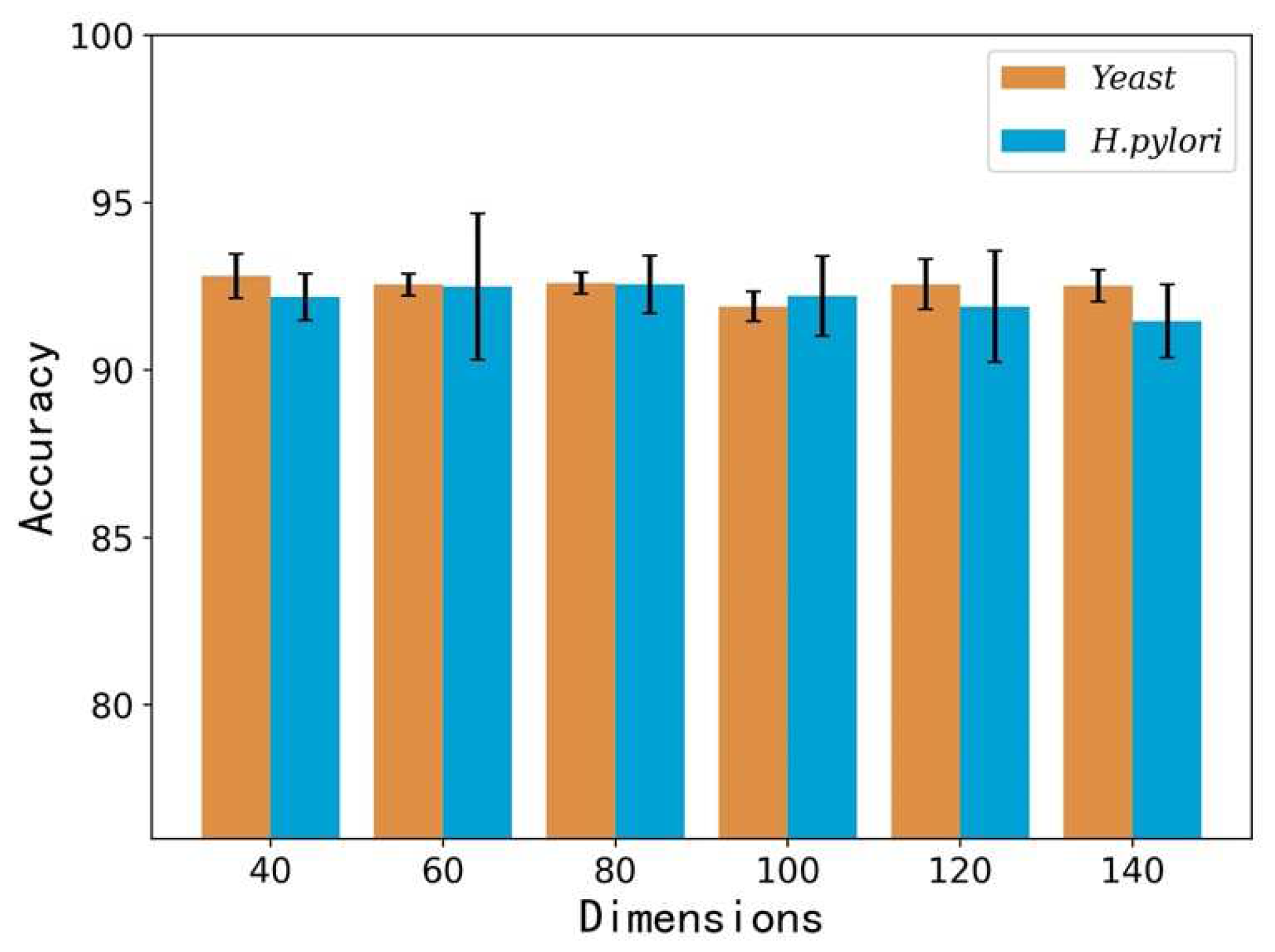
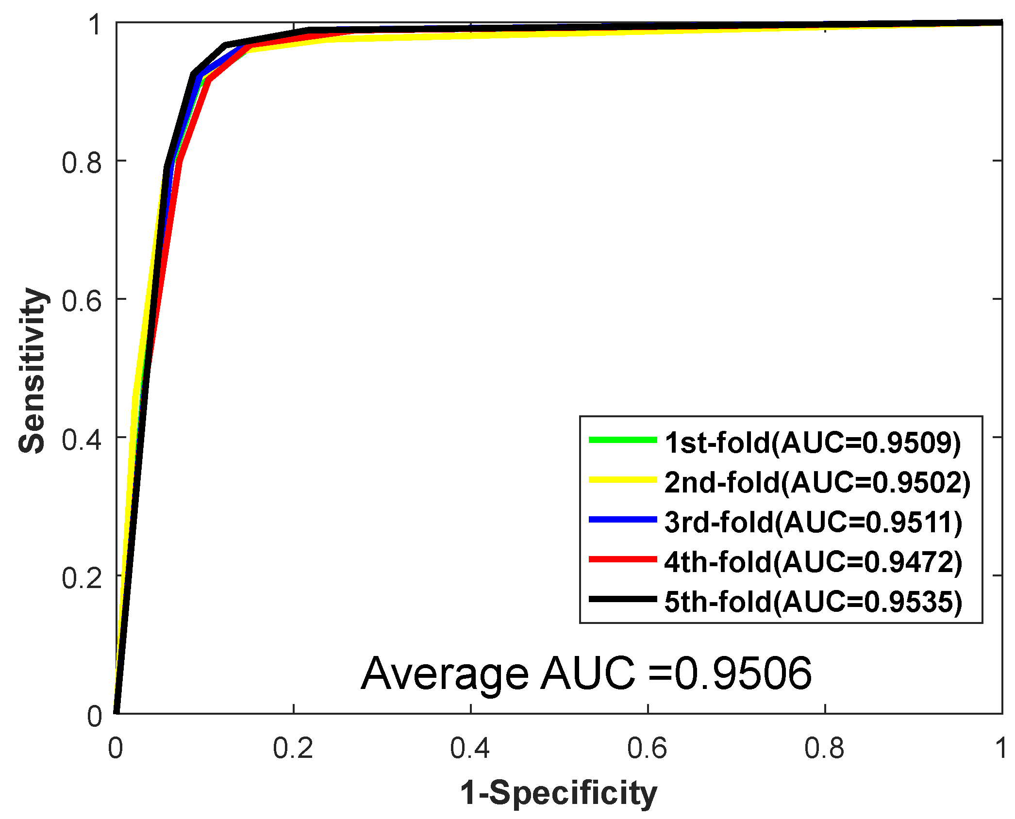
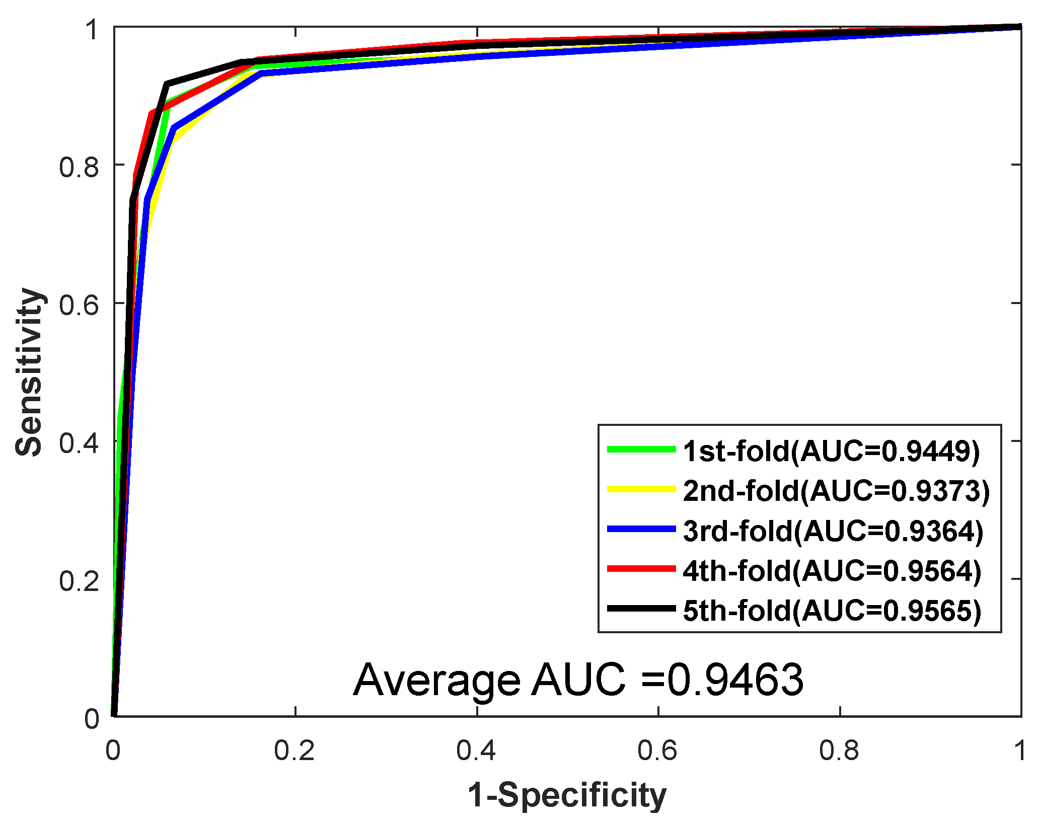
3.2. Prediction Ability Assess

In this section, we carried out our proposed method on two datasets: Yeast and H. pylori. Meanwhile, the 5-fold cross-validation method is also adopted to assess the reported method and avoid over-fitting in the experiments. By doing this, five training models would be generated on five groups of training datasets. To obtain the best feature vector representation in the LPP algorithm, we implement a variety of feature vectors with different dimensions (40-dimensional, 60-dimensional, 80-dimensional, 100-dimensional, 120-dimensional, and 140-dimensional) to predict protein interactions to obtain the best feature representation. We repeat this experiment several times and the optimization results can be seen in

Table 1. The results of different feature vectors on the Yeast and H. pylori datasets.

Feature Vectors	Dataset	Acc. (%)	Prec. (%)	Sen. (%)	MCC. (%)
40	Yeast	92.81 ± 0.66	96.80 ± 0.68	88.55 ± 0.95	86.61 ± 1.15
	H. pylori	92.18 ± 0.70	93.66 ± 2.21	90.56 ± 1.52	85.54 ± 1.15
60	Yeast	92.55 ± 0.32	96.56 ± 0.53	88.25 ± 0.81	86.16 ± 0.31
	H. pylori	92.49 ± 2.18	94.59 ± 2.13	90.12 ± 2.59	86.16 ± 3.67
80	Yeast	92.60 ± 0.32	96.37 ± 0.55	88.51 ± 0.54	86.23 ± 0.57
	H. pylori	92.56 ± 0.86	94.11 ± 0.99	90.82 ± 0.93	86.22 ± 1.47
100	Yeast	91.90 ± 0.44	94.94 ± 0.90	88.52 ± 0.46	85.08 ± 0.73
	H. pylori	92.21 ± 1.19	94.10 ± 1.74	90.12 ± 2.31	85.63 ± 2.03
120	Yeast	92.56 ± 0.75	96.44 ± 0.79	88.40 ± 0.93	86.19 ± 1.27
	H. pylori	91.90 ± 1.66	93.94 ± 1.14	89.56 ± 2.56	85.14 ± 2.81
140	Yeast	92.52 ± 0.48	95.96 ± 0.32	88.77 ± 0.79	86.12 ± 0.81
	H. pylori	91.46 ± 1.09	92.74 ± 2.54	89.89 ± 1.84	84.34 ± 1.84

. When adopting 40-dimensional feature vectors in the Yeast dataset, the result of accuracy achieved 92.81%, and when employing 80-dimensional feature vectors in the H. pylori dataset, the result of accuracy yielded 92.56%. We also plotted the accuracy performance of the Yeast and H. pylori datasets in Figure 1, which clearly illustrate that the best performance can be obtained by using 40-dimensional feature vectors on Yeast dataset and 80-dimensional feature vectors on the H. Pylori dataset. However, it is worth noting that there has been a decrease from 80-dimensional to 100-dimensional in the Yeast dataset. We thought that when we extract feature vectors from PSSM, 100-dimensional feature vectors have more redundant and noise information than 80-dimensional feature vectors. The accuracy gap between 80-dimensional and 100-dimensional is 0.70%. Moreover, the accuracy score is the main criteria we focused on. Thus, 40-dimensional feature vectors are selected on the Yeast dataset and 80-dimensional feature vectors are adopted on the H. pylori dataset.

In the rotation forest algorithm, there are two main parameters in the rotation forest classifier: K and L. where K represents the number of feature subsets, L denotes the number of decision trees. We select the best parameter after the experiment and set K, L as 5, 5, respectively. The results of the two datasets were shown in

Table 2. Prediction performance of the Yeast dataset based on five-fold cross-validation method.

Testing Set	Acc. (%)	Prec. (%)	Sen. (%)	MCC. (%)	AUC
1	92.58	97.34	88.14	86.23	0.9509
2	92.80	96.24	88.78	86.58	0.9502
3	92.85	97.39	88.35	86.68	0.9511
4	92.00	95.91	87.44	85.20	0.9472
5	93.83	97.13	90.02	88.37	0.9535
Average	92.81 ± 0.66	96.80 ± 0.68	88.55 ± 0.95	86.61 ± 1.15	0.9506 ± 0.0023

and

Table 3. Prediction performance of the H. pylori dataset based on five-fold cross-validation method.

Testing Set	Acc. (%)	Prec. (%)	Sen. (%)	MCC. (%)	AUC
1	92.80	93.50	91.52	86.61	0.9449
2	91.77	93.19	89.97	84.87	0.9373
3	91.60	93.49	90.10	84.59	0.9364
4	93.65	95.02	92.07	88.10	0.9564
5	92.97	95.32	90.44	86.91	0.9565
Average	92.56 ± 0.86	94.11 ± 0.99	90.82 ± 0.93	86.22 ± 1.47	0.9463 ± 0.0098

.

When predicting the PPIs of the Yeast dataset, the proposed method yielded results of average accuracy is 92.81%, precision is 96.80%, sensitivity is 88.55%, and MCC is 86.61%, respectively. The corresponding standard deviations are 0.66%, 0.68%, 0.95%, and 1.15%, respectively. When predicting the H. pylori, the average accuracy, precision, sensitivity, and MCC are 92.56%, 94.11%, 90.82%, and 86.22%, with the corresponding standard deviations of 0.86%, 0.99%, 0.93%, and 1.47%, respectively. Meanwhile, the values of AUC were also computed. The ROC curves of the two datasets are shown in Figure 2 and Figure 3. As shown in Figure 2 and Figure 3, for the dataset Yeast, the AUC value is 0.9506. For the dataset H. pylori, we could clearly see that the AUC value is 0.9463. In conclusion, promising results demonstrate that the method we proposed is stable and effective for predicting PPIs.

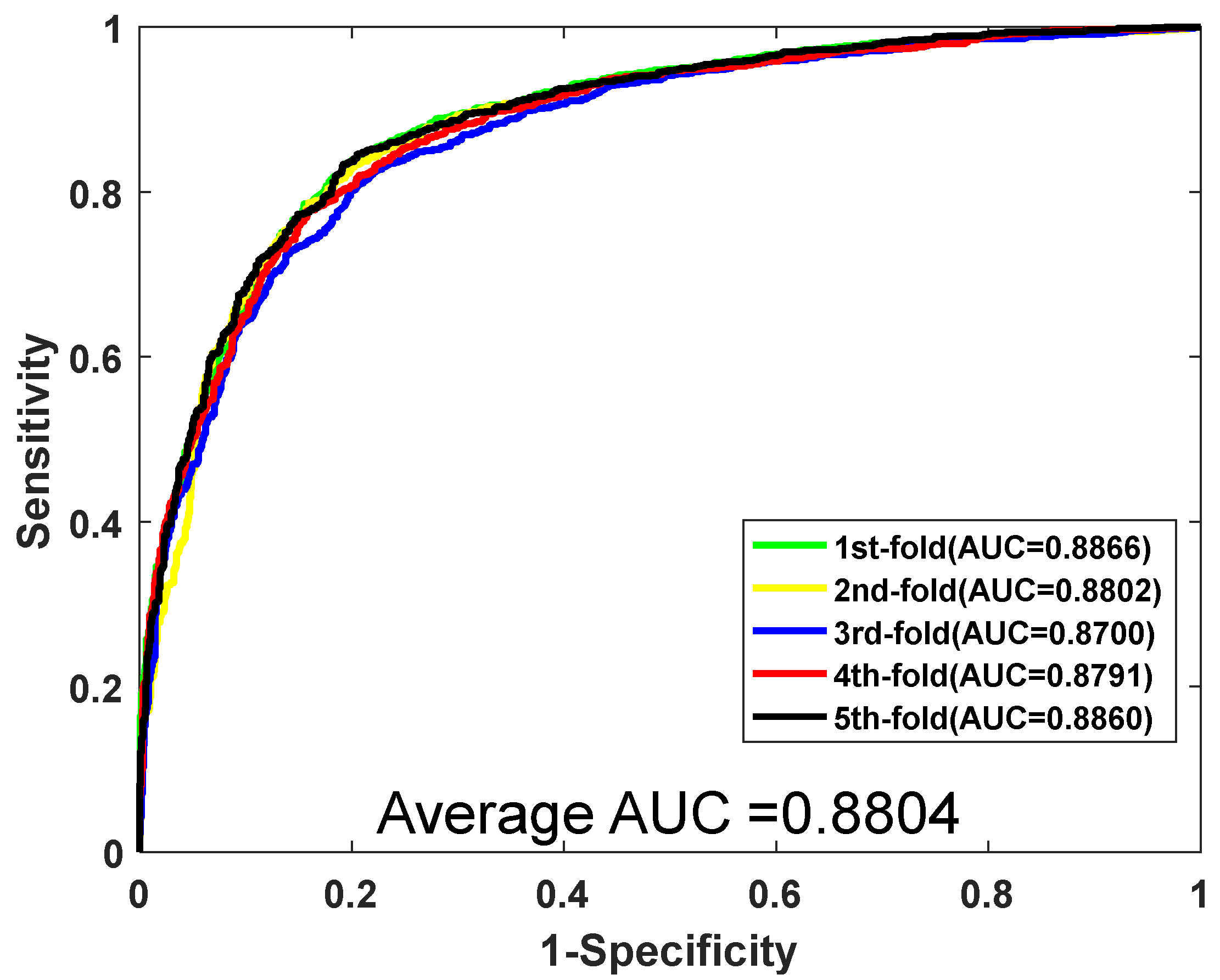
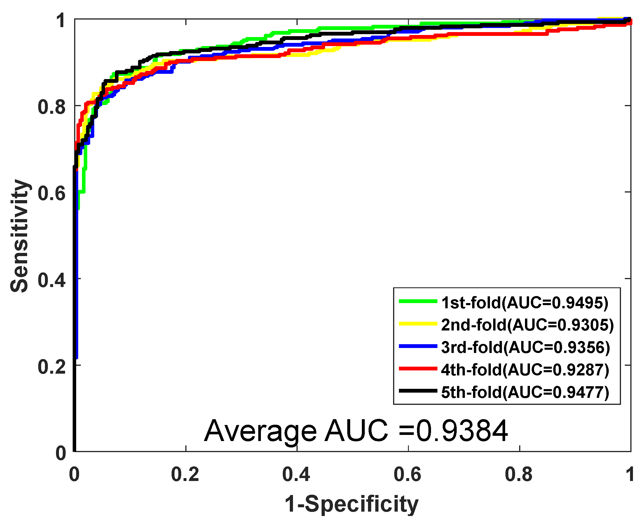
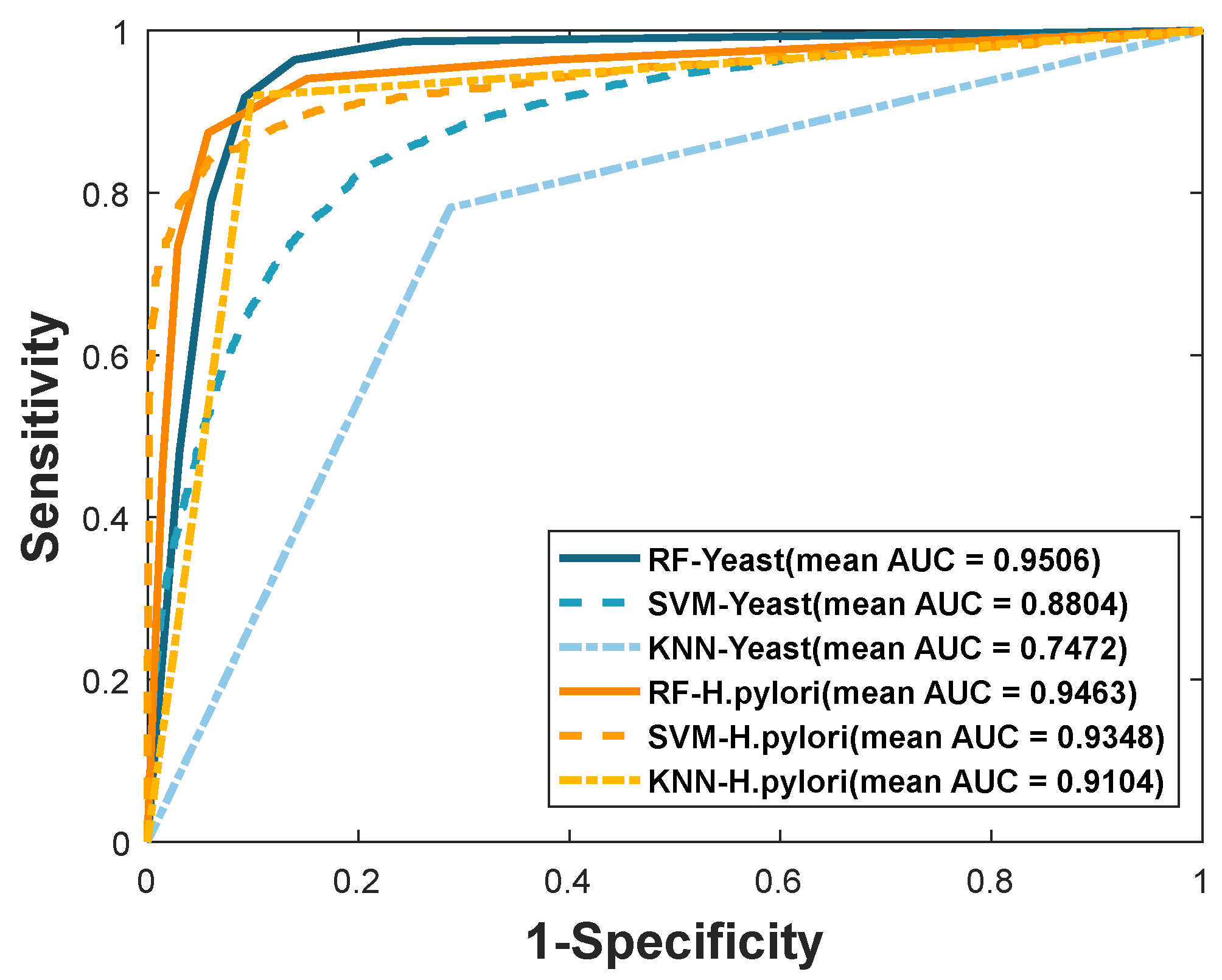
3.3. Performance Comparison of RF with Other Models

We compare the proposed method with K nearest neighbor (KNN) and support vector machine (SVM) classifier for further evaluating the proposed method. The algorithm of KNN is widely used in machine learning due to its efficiency and simplicity. The parameter k of KNN needs to be optimized to obtain the best performance. Here, the k is set to 2. When training the SVM model, the LIBSVM tool is adopted to predict PPIs. There are two corresponding parameters of c and g that need to be optimized in the SVM classifier. When we carried out the experiment using the same feature vectors, 40-dimensions in Yeast and 80-dimensions in H. pylori, in the SVM classifier, we optimized several parameters to find the best performance of the classifier. Thus, in the Yeast dataset, parameters c and g are set 1 and 4. In the H. pylori dataset, we optimize the parameter and finally, we set c = 5 and g = 0.1, respectively. The performance results of SVM can be seen in

Table 4. Prediction performance of the Yeast dataset based on five-fold cross-validation method.

Testing Set	Acc. (%)	Prec. (%)	Sen. (%)	MCC. (%)	AUC
1	81.27	83.41	79.90	69.53	0.8866
2	81.18	81.28	80.02	69.42	0.8802
3	79.48	80.85	78.37	67.37	0.8700
4	80.33	80.54	79.07	68.37	0.8791
5	81.36	80.88	80.95	69.65	0.8860
Average	80.72 ± 0.81	81.39 ± 1.16	79.66 ± 0.98	68.87 ± 0.98	0.8804 ± 0.0067

and

Table 5. Prediction performance of H. pylori dataset based on five-fold cross-validation method.

Testing Set	Acc. (%)	Prec. (%)	Sen. (%)	MCC. (%)	AUC
1	88.16	88.21	87.28	79.11	0.9495
2	89.37	92.83	85.12	80.91	0.9305
3	87.65	90.81	84.82	78.32	0.9356
4	88.85	94.47	82.41	80.02	0.9287
5	89.54	92.96	85.67	81.21	0.9477
Average	88.71 ± 0.80	91.86 ± 2.42	85.06 ± 1.76	79.91 ± 1.21	0.9384 ± 0.0097

. When using SVM for predicting the Yeast PPI dataset, the performance result of average accuracy is 80.72%, precision is 81.39%, sensitivity is 79.66%, MCC is 68.87%, and AUC becomes 0.8804, respectively. The corresponding standard deviations are 0.81%, 1.16%, 0.98%, 0.98%, and 0.0067, respectively. When the SVM is adopted to predict H. pylori, the prediction results of average accuracy, precision, sensitivity, MCC, and AUC are 88.71%, 91.86%, 85.06%, 79.91%, and 0.9438, respectively. The ROC curves of the SVM classifier on the Yeast and H. pylori datasets are shown in Figure 4 and Figure 5.

Furthermore, the prediction experiment of KNN has been carried out and the average results are obtained by adopting the same feature extraction method.

Table 6. The experimental results compared with other prediction models in the Yeast and H. pylori datasets.

Dataset	Model	Accu. (%)	Prec. (%)	Sen. (%)	MCC. (%)	AUC
Yeast	RF	92.81 ± 0.66	96.80 ± 0.68	88.55 ± 0.95	86.61 ± 1.15	0.9506 ± 0.0023
	SVM	80.72 ± 0.81	81.39 ± 1.16	79.66 ± 0.98	68.87 ± 0.98	0.8804 ± 0.0067
	KNN	74.73 ± 1.38	76.57 ± 2.18	71.28 ± 1.18	62.15 ± 1.31	0.7472 ± 0.0139
H. pylori	RF	92.56 ± 0.86	94.11 ± 0.99	90.82 ± 0.93	86.22 ± 1.47	0.9463 ± 0.0098
	SVM	88.71 ± 0.80	91.86 ± 2.42	85.06 ± 1.76	79.91 ± 1.21	0.9384 ± 0.0097
	KNN	91.05 ± 1.01	91.85 ± 1.72	90.12 ± 0.94	83.70 ± 1.64	0.9104 ± 0.0101

summarizes the prediction result of the different prediction models. The results of RF are significantly better than SVM and KNN on the Yeast dataset. For example, the accuracy gaps between RF and SVM are 12.09% in the Yeast dataset and 3.85% in the H. pylori dataset. Similarly, the accuracy gaps between RF and KNN are 18.08% in the Yeast dataset and 1.51% in the H. pylori dataset. As a result, we can conclude that the RF classifier is more accurate and outstanding than SVM and KNN.

To evaluate the method performance more intuitively, we plotted the ROC curves of RF, SVM, and KNN, which can be seen in Figure 6. It can be known that the higher the AUC value, the better the performance of the experimental method. For instance, the AUC values gaps between RF and SVM are 0.0702 in the Yeast dataset and 0.0025 in the H. pylori dataset. Similarly, the AUC values gaps between RF and KNN are 0.2034 in the Yeast dataset and 0.0359 in the H. pylori dataset.

Given more thinking in this section, we adopt the same feature vectors in different classifiers: KNN, SVM, and RF. SVM shows many unique advantages in solving small samples and nonlinear and high-dimensional pattern recognition. It always shows the state-of-the-art performance in many previous works. In addition, KNN is a commonly supervised learning method in which K is usually selected manually. In this study, RF obtained better accuracy results than KNN and SVM; it also demonstrates when predicting the protein–protein interactions, RF can capture more useful information and have less noise influence than SVM and KNN. Thus, we conclude that the method we proposed has better prediction performance for predicting PPIs.

3.4. Performance on Independent Dataset

Although our method has achieved satisfactory results, we carried out an extensive experiment on our proposed method. Four independent PPI datasets, including H. pylori, H. sapiens, C. elegans, and M. musculus, were selected to evaluate the predictive capacity of the proposed model. The experiment is based on the hypothesis that a large number of interacting proteins in an organism evolve in a related way, and their respective orthologs in other organisms also interact. Specially, we first adopted the Yeast PPI dataset as the training set after optimizing the parameters. The same feature extraction method was applied to four independent PPI datasets, and then these feature vectors of the independent dataset would be treated as test data. The results are summarized in

Table 7. Prediction results were obtained on four independent datasets.

Species	Test Pairs	Accu. (%)
H. sapiens	1412	88.60
M. musculus	313	97.44
H. pylori	1420	94.44
C. elegans	4013	93.60

.

When applying our proposed method to predict PPIs on four cross-species, we achieved the average values of accuracy varying from 88.60% to 97.44% in Table 7. Moreover, based on our hypothesis, the accuracy result for the H. sapiens dataset is 88.60% and 97.44% for M. musculus dataset. We can suppose that when we employ the Yeast dataset as the training set, the H. sapiens dataset shows a lower correlation; on the contrary, the M. musculus dataset shows a higher correlation. All in all, it demonstrates that our proposed model has good predictive and generalization capabilities in predicting PPIs and can be applied to different protein interaction prediction problems.

3.5. Comparison with Other Methods

There have been proposed many related works for improving the prediction performance. To compare whether our method is efficient or not, we make a comparison between our method and the previous works on the Yeast and H. pylori PPI datasets.

Table 8. Comparison results of different methods on H. pylori.

Model	Acc. (%)	Prec. (%)	Sen. (%)	MCC. (%)
Ensemble of HKNN [47]	86.60	85.00	86.70	N/A
HKNN [48]	84.00	84.00	86.00	N/A
Ensemble ELM [49]	87.50	88.95	86.15	78.13
Signature products [40]	83.40	85.70	79.90	N/A
Phylogenetic bootstrap [50]	75.80	80.20	69.80	N/A
Boosting [51]	79.52	81.69	80.37	70.64
Proposed method	92.56	94.11	90.82	86.22

and

Table 9. Comparison results of different methods on Yeast.

Method	Model	Acc. (%)	Prec. (%)	Sen. (%)	MCC. (%)
You’s work [49]	PCA-EELM	87.00 ± 0.29	87.59 ± 0.32	86.15 ± 0.43	77.36 ± 0.44
Zhou’s work [52]	SVM+LD	88.56 ± 0.33	89.50 ± 0.60	87.37 ± 0.22	77.15 ± 0.68
Yang’s work [53]	Cod1	75.08 ± 1.13	74.75 ± 1.23	75.81 ± 1.20	N/A
	Cod2	80.04 ± 1.06	95.44 ± 0.30	96.25 ± 1.26	N/A
	Cod3	80.41 ± 0.47	65.50 ± 1.44	97.90 ± 1.06	N/A
	Cod4	86.15 ± 1.17	90.24 ± 1.34	81.03 ± 1.74	N/A
Guo’s work [54]	ACC	89.33 ± 2.67	88.87 ± 6.16	89.93 ± 3.68	N/A
	AC	87.36 ± 1.38	87.82 ± 4.33	87.30 ± 4.68	N/A
Proposed method	RF	92.81 ± 0.66	96.80 ± 0.68	88.55 ± 0.95	86.61 ± 1.15

list the comparison result on two datasets.

Table 8 clearly illustrates that our proposed method achieved the best results in accuracy, precision, sensitivity, and MCC, respectively. Especially in the criteria of the MCC, our method is 8.09% higher than the ensemble ELM method, and our model is 5.06% higher in accuracy than ensemble ELM. Generally, the result of our method is ranked first that our model obtained the highest prediction accuracy on the H. pylori.

In Table 9, the results of previous work are listed. Our approach achieved the highest result in several criteria. Specifically, the proposed method achieved 92.81% on accuracy, which is 3.48% higher than the first highest in Guo’s work. The results yielded from our model on sensitivity only achieved 88.55%, which was 9.35% lower than the third-highest in Yang’s work. It is worth noting that the feature extraction method and classifier make a great contribution to achieving excellent performance. Generally speaking, the performance of the method we proposed is superior to other methods in the table and is effective in predicting PPIs.

4. Conclusions

In this article, we reported a novel computational method by combining locality-preserving projections and rotation forest for inferring potential PPIs. It is worth noting that the feature extraction method is conducive to predicting PPIs. The main improvement in this work is that the locality preserving projections (LPP) are insensitive to anisotropic values and can better maintain fixed local structure information internally. Then obtaining the final prediction result by employing rotation forest. The method achieved an average prediction accuracy of 92.81% on Yeast and 92.56% on H. pylori. We also further compare the prediction performance among the rotation forest, support vector machine, and K nearest neighbor. Extensive experiments were also carried out on four independent datasets. The experiment results show that the performance of our model is appropriate. However, the computational method still has some drawbacks, the feature vectors extracted by LPP have potential noise, and evolutionary information cannot be retained completely. In future studies, we will continue to study the use of more efficient descriptors to predict PPIs.

References

1. Wang, L.; You, Z.H.; Chen, X.; Li, J.Q.; Yan, X.; Zhang, W.; Huang, Y.A. An ensemble approach for large-scale identification of protein-protein interactions using the alignments of multiple sequences. Oncotarget 2017, 8, 5149–5159. [Google Scholar] [CrossRef] [Green Version]
2. Braun, P.; Gingras, A.C. History of protein-protein interactions: From egg-white to complex networks. Proteomics 2012, 12, 1478–1498. [Google Scholar] [CrossRef]
3. Takashi, I.; Tomoko, C.; Ritsuko, O.; Mikio, Y.; Masahira, H.; Yoshiyuki, S. A comprehensive two-hybrid analysis to explore the yeast protein interactome. Proc. Natl. Acad. Sci. USA 2001, 98, 4569–4574. [Google Scholar]
4. Tarassov, K.; Messier, V.; Landry, C.R.; Radinovic, S.; Molina, M.M.S.; Shames, I.; Malitskaya, Y.; Vogel, J.; Bussey, H.; Michnick, S.W. An in Vivo Map of the Yeast Protein Interactome. Science 2008, 320, 1465–1470. [Google Scholar] [CrossRef] [Green Version]
5. Zhu, H.; Snyder, M. Protein chip technology. Curr. Opin. Chem. Biol. 2003, 7, 55–63. [Google Scholar] [CrossRef]
6. Gavin, A.C.; Bosche, M.; Krause, R.; Grandi, P.; Marzioch, M.; Bauer, A.; Schultz, J.; Rick, J.M.; Michon, A.M.; Cruciat, C.M.; et al. Functional organization of the yeast proteome by systematic analysis of protein complexes. Nature 2002, 415, 141–147. [Google Scholar] [CrossRef]
7. Bader, G.D.; Doron, B.; Hogue, C.W. BIND: The biomolecular interaction network database. Nucleic Acids Res. 2003, 31, 248–250. [Google Scholar] [CrossRef]
8. Xenarios, I.; Salwinski, L.; Duan, X.J.; Higney, P.; Kim, S.M.; Eisenberg, D. DIP, the Database of Interacting Proteins: A research tool for studying cellular networks of protein interactions. Nucleic Acids Res. 2002, 30, 303–305. [Google Scholar] [CrossRef] [Green Version]
9. Licata, L.; Briganti, L.; Peluso, D.; Perfetto, L.; Iannuccelli, M.; Galeota, E.; Sacco, F.; Palma, A.; Nardozza, A.P.; Santonico, E.; et al. MINT, the molecular interaction database: 2012 update. Nucleic Acids Res. 2012, 40, D857–D861. [Google Scholar] [CrossRef]
10. Zhu, L.; You, Z.H.; Huang, D.S.; Wang, B. T-LSE: A Novel Robust Geometric Approach for Modeling Protein-Protein Interaction Networks. PLoS ONE 2013, 8, e58368. [Google Scholar] [CrossRef] [Green Version]
11. Cui, G.Y.C.; Chen, Y.; Huang, D.S.; Han, K. An algorithm for finding functional modules and protein complexes in protein-protein interaction networks. J. Biomed. Biotechnol. 2008, 2008, 860270. [Google Scholar] [CrossRef] [PubMed] [Green Version]
12. Xia, J.F.; Zhao, X.M.; Huang, D.S. Predicting protein-protein interactions from protein sequences using meta predictor. Amino Acids 2010, 39, 1595–1599. [Google Scholar] [CrossRef] [PubMed]
13. Li, J.J.; Huang, D.S.; Wang, B.; Chen, P. Identifying Protein-Protein Interfacial Residues in Heterocomplexes Using Residue Conservation Scores. Int. J. Biol. Macromol. 2006, 38, 241–247. [Google Scholar] [CrossRef] [PubMed]
14. Shi, M.G.; Xia, J.F.; Li, X.L.; Huang, D.S. Predicting protein-protein interactions from sequence using correlation coefficient and high-quality interaction dataset. Amino Acids 2010, 38, 891–899. [Google Scholar] [CrossRef]
15. Chen, P.; Wang, B.; Wong, H.S.; Huang, D.S. Prediction of protein B-factors using multi-class bounded SVM. Protein Pept. Lett. 2007, 14, 185–190. [Google Scholar] [CrossRef]
16. Zhao, X.M.; Cheung, Y.M.; Huang, D.S. A novel approach to extracting features from motif content and protein composition for protein sequence classification. Neural Netw. 2005, 18, 1019–1028. [Google Scholar] [CrossRef]
17. Zhu, L.; Deng, S.P.; You, Z.H.; Huang, D.S. Identifying spurious interactions in the protein-protein interaction networks using local similarity preserving embedding. IEEE/ACM Trans. Comput. Biol. Bioinform. 2017, 14, 345–352. [Google Scholar] [CrossRef]
18. Bao, W.Z.; Yuan, C.A.; Zhang, Y.H.; Han, K.; Nandi, A.K.; Honig, B.; Huang, D.S. Mutli-features prediction of protein translational modification sites. IEEE/ACM Trans. Comput. Biol. Bioinform. 2018, 15, 1453–1460. [Google Scholar] [CrossRef] [Green Version]
19. Xia, J.F.; Zhao, X.M.; Song, J.N.; Huang, D.S. APIS: Accurate prediction of hot spots in protein interfaces by combining protrusion index with solvent accessibility. BMC Bioinform. 2010, 11, 174. [Google Scholar] [CrossRef] [Green Version]
20. Wang, Y.B.; You, Z.H.; Li, L.P.; Huang, D.S.; Zhou, F.F.; Yang, S. Improving prediction of self-interacting proteins using stacked sparse auto-encoder with PSSM profiles. Int. J. Biol. Sci. 2018, 14, 983–991. [Google Scholar] [CrossRef]
21. Deng, S.P.; Huang, D.S. SFAPS: An R package for structure/function analysis of protein sequences based on informational spectrum method. Methods 2014, 69, 207–212. [Google Scholar] [CrossRef] [PubMed]
22. Huang, D.S.; Zhang, L.; Han, K.; Deng, S.P.; Yang, K.; Zhang, H.B. Prediction of protein-protein interactions based on protein-protein correlation using least squares regression. Curr. Protein Pept. Sci. 2014, 15, 553–560. [Google Scholar] [CrossRef] [PubMed]
23. Wang, B.; Huang, D.S.; Jiang, C.J. A new strategy for protein interface identification using manifold learning method. IEEE Trans. Nano-Biosci. 2014, 13, 118–123. [Google Scholar] [CrossRef] [PubMed]
24. Lei, Y.K.; You, Z.H.; Ji, Z.; Zhu, L.; Huang, D.S. Assessing and predicting protein interactions by combining manifold embedding with multiple information integration. BMC Bioinform. 2012, 13, 1–18. [Google Scholar] [CrossRef] [PubMed] [Green Version]
25. You, Z.H.; Lei, Y.K.; Huang, D.S.; Zhou, X.B. Using manifold embedding for assessing and predicting protein interactions from high-throughput experimental data. Bioinformatics 2010, 26, 2744–2751. [Google Scholar] [CrossRef] [Green Version]
26. Alguwaizani, S.; Park, B.; Zhou, X.; Huang, D.S.; Han, K. Predicting interactions between virus and host proteins using repeat patterns and composition of amino acids. J. Healthc. Eng. 2018, 2018, 1391265. [Google Scholar] [CrossRef] [Green Version]
27. Yi, H.C.; You, Z.H.; Huang, D.S.; Li, X.; Jiang, T.H.; Li, L.P. A deep learning framework for robust and accurate prediction of ncRNA-protein interactions using evolutionary information. Mol. Ther. Nucleic Acids 2018, 11, 337–344. [Google Scholar] [CrossRef] [Green Version]
28. Huang, D.S.; Zhao, X.M.; Huang, G.B.; Cheung, Y.M. Classifying protein sequences using hydropathy blocks. Pattern Recognit. 2006, 39, 2293–2300. [Google Scholar] [CrossRef]
29. Wang, B.; Chen, P.; Huang, D.S.; Li, J.J.; Lok, T.M.; Lyu, M.R. Predicting protein interaction sites from residue spatial sequence profile and evolution rate. FEBS Lett. 2006, 580, 380–384. [Google Scholar] [CrossRef] [Green Version]
30. Zhao, X.M.; Huang, D.S.; Cheung, Y.M. A novel hybrid GA/RBFNN technique for protein classification. Protein Pept. Lett. 2005, 12, 383–386. [Google Scholar] [CrossRef]
31. Wang, B.; Wong, H.S.; Huang, D.S. Inferring protein-protein interacting sites using residue conservation and evolutionary information. Protein Pept. Lett. 2006, 13, 999–1005. [Google Scholar] [CrossRef] [PubMed]
32. Xia, J.F.; Han, K.; Huang, D.S. Sequence-based prediction of protein-protein interactions by means of rotation forest and autocorrelation descriptor. Protein Pept. Lett. 2010, 17, 137–145. [Google Scholar] [CrossRef] [PubMed]
33. Shen, J.; Zhang, J.; Luo, X.; Zhu, W.; Yu, K.; Chen, K.; Li, Y.; Jiang, H. Predicting protein–protein interactions based only on sequences information. Proc. Natl. Acad. Sci. USA 2007, 104, 4337–4341. [Google Scholar] [CrossRef] [Green Version]
34. You, Z.H.; Zhu, L.; Zheng, C.H.; Yu, H.J.; Deng, S.P.; Ji, Z. Prediction of protein-protein interactions from amino acid sequences using a novel multi-scale continuous and discontinuous feature set. BMC Bioinform. 2014, 15, S9. [Google Scholar] [CrossRef] [Green Version]
35. Chen, C.; Zhang, Q.; Yu, B.; Yu, Z.; Lawrence, P.J.; Ma, Q.; Zhang, Y. Improving protein-protein interactions prediction accuracy using XGBoost feature selection and stacked ensemble classifier. Comput. Biol. Med. 2020, 123, 103899. [Google Scholar] [CrossRef] [PubMed]
36. Zhao, L.J.; Yuan, D.C.; Chai, T.Y.; Tang, J. KPCA and ELM ensemble modeling of wastewater effluent quality indices. Procedia Eng. 2011, 15, 5558–5562. [Google Scholar] [CrossRef] [Green Version]
37. Yousef, A.; Charkari, N.M. A novel method based on new adaptive LVQ neural network for predicting protein–protein interactions from protein sequences. J. Theor. Biol. 2013, 336, 231–239. [Google Scholar] [CrossRef]
38. Wang, T.; Li, L.; Huang, Y.A.; Zhang, H.; Ma, Y.; Zhou, X. Prediction of protein-protein interactions from amino acid sequences based on continuous and discrete wavelet transform features. Molecules 2018, 23, 823. [Google Scholar] [CrossRef] [Green Version]
39. Zahiri, J.; Yaghoubi, O.; Mohammad-Noori, M.; Ebrahimpour, R.; Masoudi-Nejad, A. PPIevo: Protein–protein interaction prediction from PSSM based evolutionary information. Genomics 2013, 102, 237–242. [Google Scholar] [CrossRef]
40. Martin, S.; Roe, D.; Faulon, J.L. Predicting protein–protein interactions using signature products. Bioinformatics 2005, 21, 218–226. [Google Scholar] [CrossRef]
41. Gribskov, M.; McLachlan, A.D.; Eisenberg, D. Profile analysis: Detection of distantly related proteins. Proc. Natl. Acad. Sci. USA 1987, 84, 4355–4358. [Google Scholar] [CrossRef] [PubMed] [Green Version]
42. Huang, C.; Yuan, J. Using radial basis function on the general form of Chou’s pseudo amino acid composition and PSSM to predict subcellular locations of proteins with both single and multiple sites. Biosystems 2013, 113, 50–57. [Google Scholar] [CrossRef] [PubMed]
43. Verma, R.; Varshney, G.C.; Raghava, G.P.S. Prediction of mitochondrial proteins of malaria parasite using split amino acid composition and PSSM profile. Amino Acids 2010, 39, 101–110. [Google Scholar] [CrossRef] [PubMed]
44. Altschul, S.F.; Madden, T.L.; Schaffer, A.A.; Zhang, J.; Zhang, Z.; Miller, W.; Lipman, D.J. Gapped BLAST and PSI-BLAST: A new generation of protein database search programs. Nucleic Acids Res. 1997, 25, 338–3402. [Google Scholar] [CrossRef] [PubMed] [Green Version]
45. He, X.; Niyogi, P. Locality preserving projections. Adv. Neural Inf. Process. Syst. 2004, 16, 153–160. [Google Scholar]
46. Rodriguez, J.J.; Kuncheva, L.I.; Alonso, C.J. Rotation forest: A new classifier ensemble method. IEEE Trans. Pattern Anal. Mach. Intell. 2006, 28, 1619–1630. [Google Scholar] [CrossRef]
47. Nanni, L.; Lumini, A. An ensemble of K-local hyperplanes for predicting protein–protein interactions. Bioinformatics 2006, 22, 1207–1210. [Google Scholar] [CrossRef]
48. Nanni, L. Hyperplanes for predicting protein–protein interactions. Neurocomputing 2005, 69, 257–263. [Google Scholar] [CrossRef]
49. You, Z.H.; Lei, Y.K.; Zhu, L.; Xia, B.; Wang, B. Prediction of protein-protein interactions from amino acid sequences with ensemble extreme learning machines and principal component analysis. BMC Bioinform. 2013, 14, S10. [Google Scholar] [CrossRef] [Green Version]
50. Bock, J.R.; Gough, D.A. Whole-proteome interaction mining. Bioinformatics 2003, 19, 125–134. [Google Scholar] [CrossRef] [Green Version]
51. Liu, B.; Yi, J.; Aishwarya, S.V.; Lan, Y.; Ma, Y.; Huang, T.H.; Leone, G.; Jin, V.X. QChIPat: A quantitative method to identify distinct binding patterns for two biological ChIP-seq samples in different experimental conditions. BMC Genom. 2013, 14, S3. [Google Scholar] [CrossRef] [PubMed] [Green Version]
52. Zhou, Y.Z.; Gao, Y.; Zheng, Y.Y. Prediction of protein-protein interactions using local description of amino acid sequence. Adv. Comput. Sci. Educ. Appl. 2011, 202, 254–262. [Google Scholar]
53. Yang, L.; Xia, J.F.; Gui, J. Prediction of protein-protein interactions from protein sequence using local descriptors. Protein Pept. Lett. 2010, 17, 1085–1090. [Google Scholar] [CrossRef] [PubMed]
54. Guo, Y.Z.; Yu, L.Z.; Wen, Z.N.; Li, M.L. Using support vector machine combined with auto covariance to predict protein-protein interactions from protein sequences. Nucleic Acids Res. 2008, 36, 3025–3030. [Google Scholar] [CrossRef] [PubMed] [Green Version]
Figure 1. The accuracy performance of the Yeast and H. pylori datasets.
Biology 11 00995 g001
Figure 2. ROC curves yielded by RF on Yeast.
Biology 11 00995 g002
Figure 3. ROC curves yielded by RF on H. pylori.
Biology 11 00995 g003
Figure 4. The ROC curve of the SVM classifier on the Yeast dataset.
Biology 11 00995 g004
Figure 5. The ROC curve of the SVM classifier on the H. pylori dataset.
Biology 11 00995 g005
Figure 6. Comparison of ROC curves for different classifiers of RF, SVM, and KNN on two datasets: Yeast and H. pylori.
Biology 11 00995 g006