Numerical Method for Coupled Nonlinear Schrödinger Equations in Few-Mode Fiber

Abstract

This paper discusses novel approaches to the numerical integration of the coupled nonlinear Schrödinger equations system for few-mode wave propagation. The wave propagation assumes the propagation of up to nine modes of light in an optical fiber. In this case, the light propagation is described by the non-linear coupled Schrödinger equation system, where propagation of each mode is described by own Schrödinger equation with other modes’ interactions. In this case, the coupled nonlinear Schrödinger equation system (CNSES) solving becomes increasingly complex, because each mode affects the propagation of other modes. The suggested solution is based on the direct numerical integration approach, which is based on a finite-difference integration scheme. The well-known explicit finite-difference integration scheme approach fails due to the non-stability of the computing scheme. Owing to this, here we use the combined explicit/implicit finite-difference integration scheme, which is based on the implicit Crank–Nicolson finite-difference scheme. It ensures the stability of the computing scheme. Moreover, this approach allows separating the whole equation system on the independent equation system for each wave mode at each integration step. Additionally, the algorithm of numerical solution refining at each step and the integration method with automatic integration step selection are used. The suggested approach has a higher performance (resolution)—up to three times or more in comparison with the split-step Fourier method—since there is no need to produce direct and inverse Fourier transforms at each integration step. The key advantage of the developed approach is the calculation of any number of modes propagated in the fiber.

1. Introduction

This article is a continuation of our previous work [1], where we suggested a novel solution of CNSES for simulation of ultra-short optical pulse propagation in birefringent fibers. The introduction of our previous work [1] completely reveals the reasons, importance, and necessity of the problem formulation. The main motive of our study was because the designers of fiber optic transmitting and receiving devices lack the tools to determine the shape of distortion of a signal that is transmitted at high power or transmitted over very long distances. Even the commonly-used split-step Fourier method, which gives quite satisfactory results, provides a general solution for the task at hand without particularities. The difference between our previous publication [1] and the current is in a number of propagation modes in the fiber. Birefringent fibers propose propagating two wave modes while few-mode fibers propose propagating up to nine modes. Our goal was to propose a method to solve the system of Schrödinger equations, which allows obtaining more detailed information on the shape of distortions of the signal propagating in the few-mode fiber under various conditions.

It is necessary to emphasize that pulse propagation in fibers with abnormal dispersion is an important investigation theme as femtosecond lasers have an influential position in industrial field [2,3,4,5]. Special optical fibers are developed for transmission of high-power ultrashort pulses [6,7] with accent to polarization maintaining fibers. The negative role of chromatic dispersion appears with increase in the length of the optical fiber communication line. The physical reason for dispersion is the frequency dependence of the phase velocity or phase delay during propagation of electromagnetic waves in the medium. This leads to a violation of the phase vectors in the wave package. When these negative effects are studied, only envelope distortion is usually considered. However, phase distortions are also important for certain classes of problems. For example, the problem of chirping during the propagation of an optical signal in an optical fiber with nonlinear dispersion is one of them.

The first part of the work is devoted to the computing of complex envelop calculations, the second is devoted to the phase velocity or phase delay calculation during the propagation of optical waves in the fibers.

2. Computing Method for Complex Envelopes of Optical Wave Calculation

2.1. CNSES for Few Modes in Dimensionless Form

The evolution of optical waves in a fiber can be described by the CNSES as:

$$\{\begin{array}{l}\frac{\partial W^{(i)}}{\partial z}=-\frac{{\alpha }^{(i)}}{2}{W}^{(i)}-{\mathsf{\beta }}_1^{(i)}\frac{\partial W^{(i)}}{\partial t}-j\frac{{\mathsf{\beta }}_2^{(i)}}{2}\frac{{\partial }^2{W}^{(i)}}{\partial t^2}+\frac{{\mathsf{\beta }}_3^{(i)}}{6}\frac{{\partial }^3{W}^{(i)}}{\partial t^3}+\\ +j{\gamma }^{(i)}{W}^{(i)}{\displaystyle \sum _{m=1}^M{C}_{i,m}{\left|W^{(m)}\right|}^2}-\frac{{\gamma }^{(i)}}{{\mathsf{\omega }}_0^{(i)}}{\displaystyle \sum _{m=1}^M{B}_{i,m}\frac{\partial }{\partial t}\left({\left|W^{(m)}\right|}^2{W}^{(i)}\right)}-j{\gamma }^{(i)}{T}_R{W}^{(i)}{\displaystyle \sum _{m=1}^M{B}_{i,m}\frac{\partial }{\partial t}\left({\left|W^{(m)}\right|}^2\right)},\\ i=\overline{1,M},\end{array}$$

(1)

with the initial and boundary conditions for each propagation mode:

$$W^{(i)}(z,0)=0, \frac{\partial W^{(i)}(z,0)}{\partial t}=0, W^{(i)}(z,T_N)=0,\forall z\in [0,L], W^{(i)}(0,t)=f^{(i)}(t), 0\le t\le T_N, i=\overline{1,M},$$

(2)

The definitions are used in Equations (1) and (2): W_i—the complex envelope of the optical wave of the i-th mode, α⁽ⁱ⁾—attenuation of the i-th mode; β⁽ⁱ⁾₁, β⁽ⁱ⁾₂, β⁽ⁱ⁾₃—the first, second and third order dispersion of the i-th mode respectively; γ⁽ⁱ⁾—parameter of nonlinearity for the i-th mode; C_i,m, B_i,m—coupling coefficients between the i-th and m-th modes; T_R—Raman scattering parameter; ω⁽ⁱ⁾₀—angular frequency of the i-th mode; z—coordinate along an optical fiber; t—time, j—imaginary one, T_N—final time, and f⁽ⁱ⁾(t)—known functions at the initial time.

To transfer Equation (1) into dimensionless form, the specific values of the process are used, namely L— length, T_N— time, and P—power, by relations:

$$\xi =z/L, \mathsf{\tau }=t/T_N, x^{(i)}=W^{(i)}/\sqrt{P},$$

(3)

Replacement of Equation (3) into Equation (1) transforms it into a dimensionless form:

$$\{\frac{\partial x^{(i)}}{\partial \xi }=-\left[a^{(i)}+\Phi 1^{(i)}\right]\cdot x^{(i)}-\left[b_1^{(i)}+\Phi 2^{(i)}\right]\cdot \frac{\partial x^{(i)}}{\partial \mathsf{\tau }}-j{b}_2^{(i)}\frac{{\partial }^2{x}^{(i)}}{\partial {\mathsf{\tau }}^2}+b_3^{(i)}\frac{{\partial }^3{x}^{(i)}}{\partial {\mathsf{\tau }}^3}, i=\overline{1,M},$$

(4)

where the dimensionless coefficients:

$$a^{(i)}=\frac{{\alpha }^{(i)}L}{2},b_1^{(i)}={\mathsf{\beta }}_1^{(i)}\frac{L}{T},b_2^{(i)}=\frac{{\mathsf{\beta }}_2^{(i)}}{2}\frac{L}{T^2},b_3^{(i)}=\frac{{\mathsf{\beta }}_3^{(i)}}{6}\frac{L}{T^3},u^{(i)}={\gamma }^{(i)}LP,v^{(i)}=\frac{u^{(i)}}{{\mathsf{\omega }}_{0}T},w^{(i)}=u^{(i)}\frac{T_R}{T_N},$$

(5)

and the definitions for the non-linear component:

$$\Phi 1^{(i)}=(v^{(i)}+j{w}^{(i)})\cdot {\displaystyle \sum _{m=1}^M{B}_{i,m}\frac{\partial }{\partial \mathsf{\tau }}\left({\left|x^{(m)}\right|}^2\right)}-j{u}^{(i)}{\displaystyle \sum _{m=1}^M{C}_{i,m}{\left|x^{(m)}\right|}^2},\Phi 2^{(i)}=v^{(i)}{\displaystyle \sum _{m=1}^M{B}_{i,m}{\left|x^{(m)}\right|}^2},$$

(6)

are used.

Equation (1) is specially separated on linear and nonlinear terms, it allows us to realize the numerical integration algorithm based on computing scheme, where all linear terms are written in implicit and all nonlinear terms are written in explicit finite-difference form.

2.2. The Finite-Difference Scheme and Computing Scheme

The Equation system (4) can be simplified by using F⁽ⁱ⁾(x) terms to denote the right parts of Equation (4):

$$\{\frac{\partial x^{(i)}}{\partial \xi }=F^{(i)}, i=\overline{1,M}.$$

(7)

The finite-difference equivalences for Equation (7), according to [1], have the form:

$$\{\frac{\left(x_{k+1,n}^{(i)}+x_{k+1,n-1}^{(i)}\right)-\left(x_{k,n}^{(i)}+x_{k,n-1}^{(i)}\right)}{2\Delta \xi }=\mathsf{\theta }\cdot F_{k+1,n-1/2}^{(i)}+(1-\mathsf{\theta })\cdot F_{k,n-1/2}^{(i)}, i=\overline{1,M}, n=\overline{3,N-1}, k=\overline{1,K},$$

(8)

where bottom index k is used to denote the mesh points along the length ξ_k = Δξ⋅(k − 1) and n is used to denote the dimensionless time mesh points τ_n = Δτ⋅(n − 1). The dimensionless parameter θ allows to attribute the value of right part of Equation (8) to an arbitrary mesh point with fractional indexes (k + θ, n − ½). The parameter θ ∈ [0, 1], defines the explicit θ = 0 or implicit θ ∈ (0, 1] finite-difference computing scheme. The recommendation for θ parameter choosing was given in [1]. There, it was approved that θ = ½, which leads to stable and reasonable results.

All variables with the k-index in Equation (8) are known as well as all variables with the (k + 1) indexes are known at n equal to 0, 1, 2, and N from Equation (2). The values of F⁽ⁱ⁾ are attributed to middleware virtual mesh points between (k+ θ, n − ½).

The nonlinearity in Φ1⁽ⁱ⁾ and Φ2⁽ⁱ⁾, and a third-order partial derivative by time in Equation (4), require modification of Crank–Nicolson’s method [1,8]. The aim is to use implicit form for linear terms, and explicit form for nonlinear ones. Thus, we separate the F⁽ⁱ⁾ on the sum of linear and nonlinear terms:

$$F_{k,n-1/2}^{(i)}=L_{k,n-1/2}^{(i)}+N_{k,n-1/2}^{(i)},$$

(9)

with the definitions for linear L⁽ⁱ⁾ and non-linear N⁽ⁱ⁾ terms at the k-layer:

$$\begin{gathered} L_{k,n-1/2}^{(i)}=-a{x}_{k,n-1/2}^{(i)}-b_1^{(i)}{\left(\frac{\partial x^{(i)}}{\partial \mathsf{\tau }}\right)}_{k,n-1/2}-j{b}_2^{(i)}{\left(\frac{{\partial }^2{x}^{(i)}}{\partial {\mathsf{\tau }}^2}\right)}_{n-1/2,k}+b_3^{(i)}{\left(\frac{{\partial }^3{x}^{(i)}}{\partial {\mathsf{\tau }}^3}\right)}_{k,n-1/2}, \\ {N}_{k,n-1/2}^{(i)}=-\Phi 1_{k,n-1/2}^{(i)}{x}_{k,n-1/2}^{(i)}-\Phi 2_{k,n-1/2}^{(i)}{\left(\frac{\partial x^{(i)}}{\partial \mathsf{\tau }}\right)}_{k,n-1/2} \end{gathered}$$

(10)

For the calculation of the linear terms L⁽ⁱ⁾ on the (k + 1)-th layer, we can just replace k on (k + 1) in Equation (10). For the nonlinear terms on (k + 1)-th layer, we must use finite-difference definition in explicit form:

$$N_{k+1,n-1/2}^{(i)}=-\Phi 1_{k,n-1/2}^{(i)}{x}_{k+1,n-1/2}^{(i)}-\Phi 2_{k,n-1/2}^{(i)}{\left(\frac{\partial x^{(i)}}{\partial \mathsf{\tau }}\right)}_{k+1,n-1/2}.$$

(11)

Hence, the explicit form in Equation (8) is used only for Φ1⁽ⁱ⁾ and Φ2⁽ⁱ⁾, while the implicit form is used for the linear terms. The nonlinear terms Φ1⁽ⁱ⁾ and Φ2⁽ⁱ⁾ in virtual grid point (k, n − ½) are written as:

$$\begin{gathered} \Phi 1_{k,n-1/2}^{(i)}=-\frac{j{u}^{(i)}}{2}{\displaystyle \sum _{m=1}^M{C}_{i,m}\left({\left|x_{k,n}^{(m)}\right|}^2+{\left|x_{k,n-1}^{(m)}\right|}^2\right)}+\frac{v^{(i)}+j{w}^{(i)}}{\Delta \mathsf{\tau }}{\displaystyle \sum _{m=1}^M{B}_{i,m}\left({\left|x_{k,n}^{(m)}\right|}^2-{\left|x_{k,n-1}^{(m)}\right|}^2\right)}, \\ \Phi 2_{k,n-1/2}^{(i)}=\frac{v^{(i)}}{2}{\displaystyle \sum _{m=1}^M{B}_{i,m}\left({\left|x_{k,n}^{(m)}\right|}^2+{\left|x_{k,n-1}^{(m)}\right|}^2\right)}. \end{gathered}$$

(12)

The desired function values in (k, n − ½) point are written as an average of two adjacent values. The partial derivative from this functions in the mentioned point can be written as central finite-differences with second-order accuracy. It gives the linear equation system for each mode at each integration step:

$$\{\begin{array}{l}\frac{x_{k+1,n}^{(i)}+x_{k+1,n-1}^{(i)}}{2\cdot \Delta \xi \cdot \mathsf{\theta }}+\frac{a+\Phi 1_{k,n-1/2}^{(i)}}{2}\left(x_{k+1,n}^{(i)}+x_{k+1,n-1}^{(i)}\right)+\frac{b_1^{(i)}+\Phi 2_{k,n-1/2}^{(i)}}{\Delta \mathsf{\tau }}\left(x_{k+1,n}^{(i)}-x_{k+1,n-1}^{(i)}\right)+\\ +\frac{j{b}_2^{(i)}}{2\Delta {\mathsf{\tau }}^2}\left(x_{k+1,n+1}^{(i)}-x_{k+1,n}^{(i)}-x_{k+1,n-1}^{(i)}+x_{k+1,n-2}^{(i)}\right)-\frac{b_3^{(i)}}{\Delta {\mathsf{\tau }}^3}\left(x_{k+1,n+1}^{(i)}-3x_{k+1,n}^{(i)}+3x_{k+1,n-1}^{(i)}-x_{k+1,n-2}^{(i)}\right)=\\ =\frac{x_{k,n}^{(i)}+x_{k,n-1}^{(i)}}{2\cdot \Delta \xi \cdot \mathsf{\theta }}+\frac{(1-\mathsf{\theta })}{\mathsf{\theta }}\left(L_{k,n-1/2}^{(i)}+N_{k,n-1/2}^{(i)}\right)\\ n=\overline{2,N-1}, i=\overline{1,M}\end{array}.$$

(13)

It is very important to note that the linear Equation system (13) for the i-th mode depends only on x⁽ⁱ⁾_k+1,n unknowns and does not depend on unknowns from other wave modes. It allows solving the linear equation system for the each i-th mode independently. The index n for each linear equation system for the i-th mode begins from 2 up to the N − 1, because the values of x_k+1,1, x_k+1,2, and x_k+1,N are known due to Equation (2).

It should be highlighted that the Equation system (13) decomposes into M independent line equation systems, according to grid node variables x⁽ⁱ⁾_k+1,n (where n begins from 3 and increases to N − 1). Each equation system can be solved separately. These linear equation systems have four-diagonal matrix form, where in addition to the main diagonal, there are one “upper” and two “sub” diagonals. We use the modified Thomas tridiagonal algorithm, which allows us to transform this matrix to triangular form. The described refinement algorithm is used at each integration step. The definition of nonlinear terms (from previous k-th integration layer) explicitly contributes to the error in calculating the values of the new (k + 1)-th layer. The main goal of the proposed refinement algorithm is to introduce iteration of the computation process at each integration step, which corrects the explicit form of nonlinear terms [1].

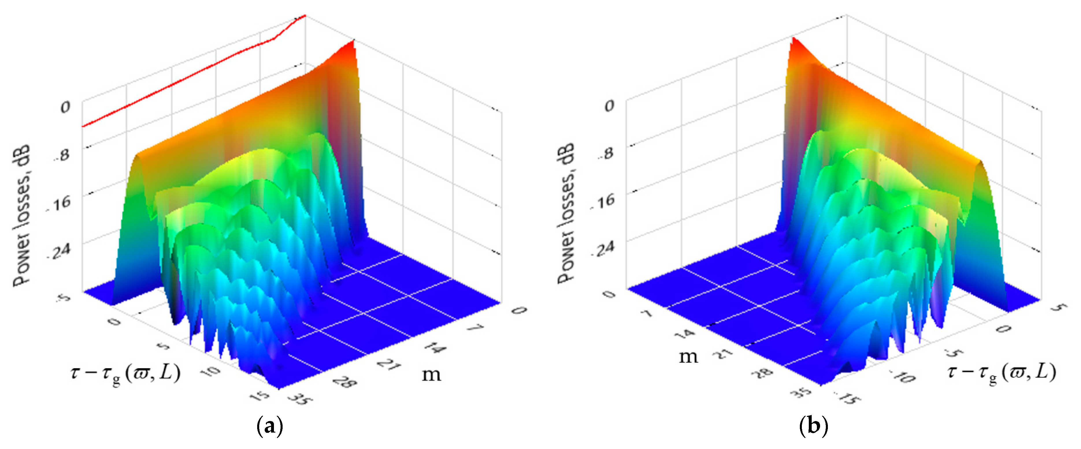
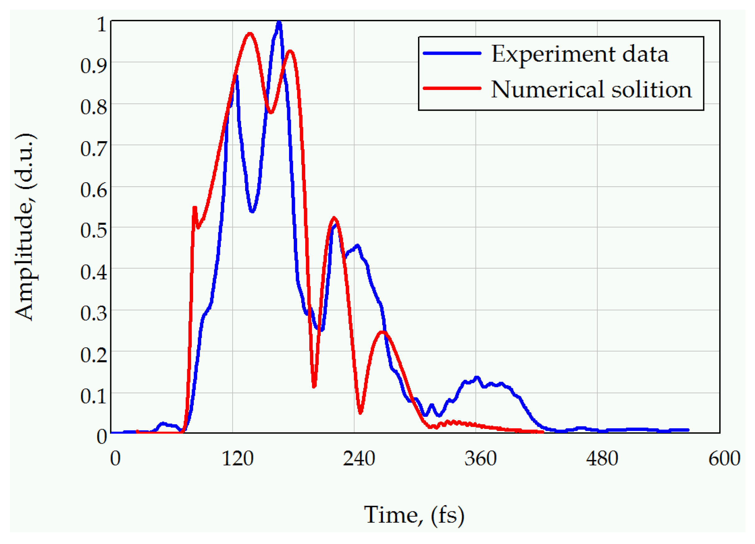
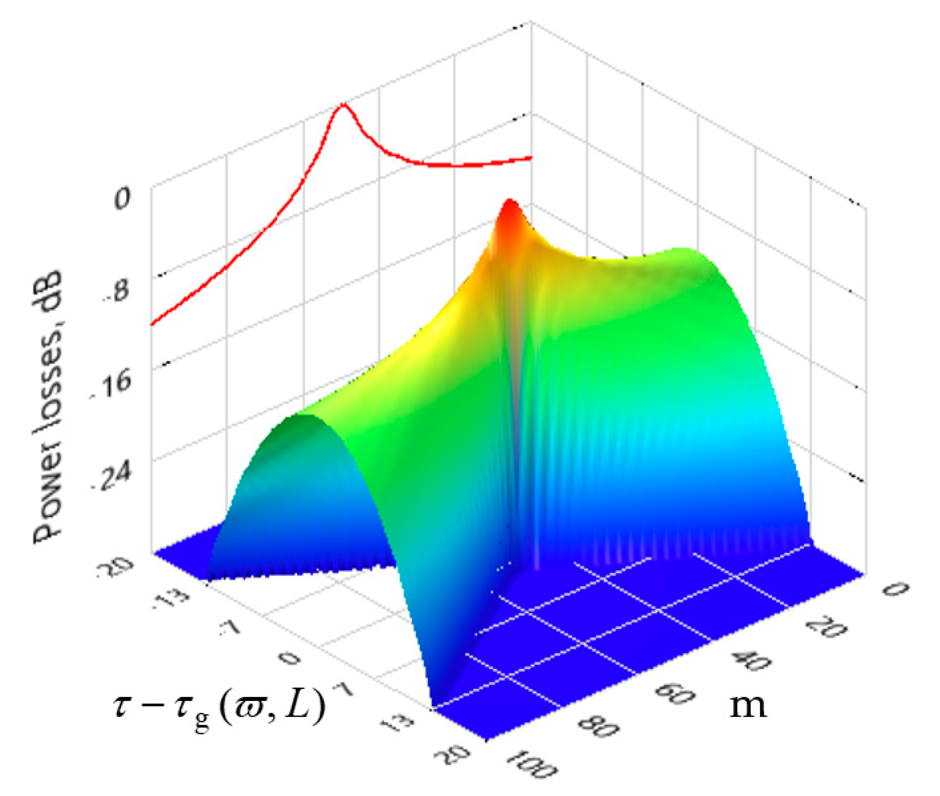
2.3. The Ultra-Short Pulse Evolution in Fiber

The ultra-short pulse propagation in optical fiber including third-order dispersion and Raman scattering is described by complete CNSES. The initial data for the calculations were taken from [9,10,11,12,13,14,15,16]: α⁽¹⁾ = α⁽²⁾ = 0.2 dB∙m/km, β⁽¹⁾ = 4.294 × 10⁻⁹ s/m, β⁽²⁾₁ = 4.290 × 10⁻⁹ s/m, β⁽¹⁾₂ = 3.600 × 10⁻²⁶ s²/m, β⁽²⁾₂ = 3.250 × 10⁻²⁶ s²/m, β⁽¹⁾₃ = β⁽²⁾ = 2.750 × 10⁻⁴¹ s³/m, γ⁽¹⁾ = γ⁽²⁾ = 3.600 × 10⁻² (m⋅W)⁻¹, T_R = 4.000 × 10⁻¹⁵ s, ω⁽¹⁾₀ = ω⁽²⁾₀ =2.3612 × 10⁻¹⁵ s⁻¹ (λ = 798 nm). The single chirped Gauss pulse (chirp C = −0.4579) was put into the fiber−s input; pulse duration is 12 fs, peak power is P = 1.75 × 10⁵ W. The pulse form is described as:

$$f(t)=A\cdot \exp \left(-\frac{(1-j\cdot C){(t-T_N)}^2}{2\cdot {\mathsf{\tau }}^2}\right).$$

(14)

20,000 grid points along dimensionless time was chosen; approximately 720,000 integration with initial step Δξ = 1∙10⁻⁴ d.u. were made. Usage of the automatic integration step correction algorithm was included, allowing to calculate the pulse evolution length up to ~2.5 mm. The maximum error was set as 10⁻³⁰ d.u. All calculations were made using a processor with double precision and 64-bit architecture.

A comparison of the pulses’ forms calculated by our method (red line) and experiment data from [9,10,11,12,13,14,15,16] is shown in Figure 1.

The numerical result (red line in Figure 1) fits well with the experimental result (blue line in Figure 1). It shows that the proposed method is effective and can be used for solving similar nonlinear tasks.

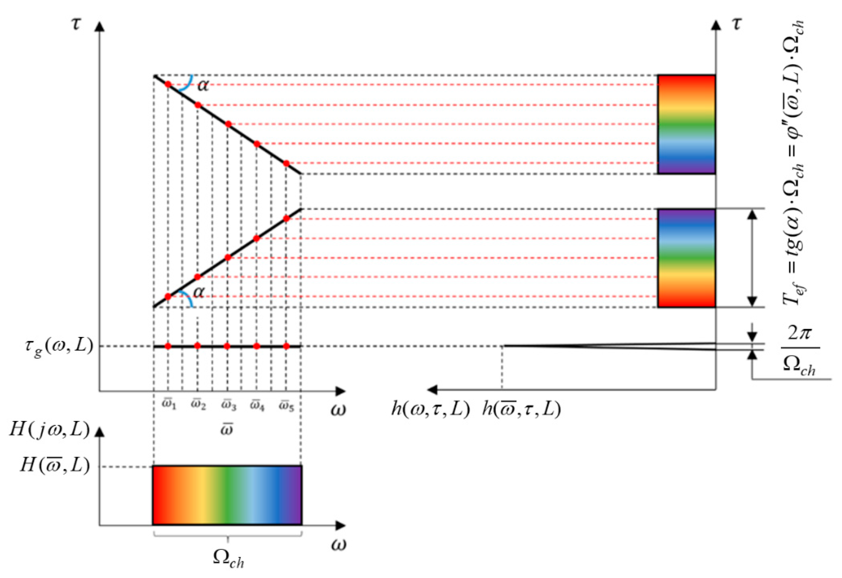
3. The Phase Velocity or Phase Delay Calculation during the Wave Propagation

Recently, the channel model, based on equivalence principle [17,18,19], was used for description of propagation of wave packages in media. According to this model, the task of wave package propagation was replaced by the task of wave package passing through line system with frequency H(jω) and h(τ) impulse characteristics:

$$\begin{gathered} H(j\mathsf{\omega },L)=\left|H(j\mathsf{\omega },L)\right|\exp \left[-j\mathsf{\phi }(\mathsf{\varpi }+\Omega ,L)\right],\mathsf{\phi }(\mathsf{\omega },L)=-Arg\left(H\left(j\mathsf{\omega },L\right)\right), \\ H(j\mathsf{\omega },L)=F\left[h(\mathsf{\tau },L)\right],h(\mathsf{\tau },L)=F^{-1}\left[H(j\mathsf{\omega },L)\right], \end{gathered}$$

(15)

where φ(ω) is phase incursion in media or phase-frequency characteristic of the line system, where the frequency set of the package ω can be presented as the sum of average ϖ and difference Ω package frequencies as ω = ϖ + Ω. The F[] and F⁻¹[] denote direct and inverse Fourier transform operator.

It is convenient to use the expression of time delays instead of velocities of propagation while studying the dispersion. Therefore, the phase delay τ_p and group delay τ_g (fast time) terms are involved into consideration, which are defined from phase-frequency characteristics of the system [20]:

$${\mathsf{\tau }}_{\mathrm{p}}(\mathsf{\omega },L)=\frac{\mathsf{\phi }(\mathsf{\omega },L)}{\mathsf{\omega }}, {\mathsf{\tau }}_{\mathrm{g}}(\mathsf{\omega },L)=\frac{\mathrm{d}\mathsf{\phi }(\mathsf{\omega },L)}{\mathrm{d}\mathsf{\omega }}.$$

(16)

The minus sign “–“ ahead of the phase φ(ω, L) of frequency characteristic in Equation (15) is introduced because the derivative of phase defines the phase delay. Group delay is a differential characteristic of phase incursion in the media (in the neighborhood of the selected frequency), and phase delay is an integrated characteristic.

The most common approach in the investigation of dispersion is related to the differential characteristic definition, where frequency characteristic covers the frequency range Ω_ch with average frequency ϖ, and amplitude-frequency and phase-frequency characteristics (Equation (15)) are presented by Taylor power series of deferential frequencies (ω − ϖ) = Ω at the ϖ average frequency point:

$$H(\mathsf{\varpi }+\Omega )\approx H(\mathsf{\varpi })\equiv const.$$

(17)

$$\mathsf{\phi }(\mathsf{\varpi }+\Omega )\approx \mathsf{\phi }(\mathsf{\varpi })+{\mathsf{\phi }}^{\prime }(\mathsf{\varpi })\cdot \Omega +\frac{1}{2}{{\mathsf{\phi }}^{\prime }}^{\prime }(\mathsf{\varpi })\cdot {\Omega }^2+\frac{1}{6}{{{\mathsf{\phi }}^{\prime }}^{\prime }}^{\prime }(\mathsf{\varpi })\cdot {\Omega }^3+\mathrm{o}({\Omega }^4),\forall \Omega \in \left[-{\Omega }_{\mathrm{ch}}/2,{\Omega }_{\mathrm{ch}}/2\right]$$

(18)

For a homogeneous medium, among which there is optical fiber, the phase-frequency characteristic is related to the refractive index of a fiber n(ω) and fiber length L by the relation:

$$\mathsf{\phi }(\mathsf{\omega },L)=\frac{L}{c}\mathsf{\omega }\cdot n(\mathsf{\omega })$$

(19)

The coefficients at frequencies in the Taylor power series of phase-frequency characteristic Equation (18) are the parameters of phase dispersion of appropriate order. Thus, the dispersion parameters evolve by increasing the length L in dispersal systems. When some critical length is achieved, dispersal distortions occur due to non-linear term effects on phase-frequency characteristic.

It is convenient to use the group phase delay as a function of frequency for phase dispersion analysis in the channel model:

$${\mathsf{\tau }}_{\mathrm{g}}(\mathsf{\varpi }+\Omega ,L)=\frac{d\mathsf{\phi }(\mathsf{\omega },L)}{d\mathsf{\omega }}={\mathsf{\tau }}_{\mathrm{g}}(\mathsf{\varpi },L)+{{\mathsf{\tau }}^{\prime }}_{\mathrm{g}}(\mathsf{\varpi },L)\cdot \Omega +\frac{1}{2}{{{\mathsf{\tau }}^{\prime }}^{\prime }}_{\mathrm{g}}(\mathsf{\varpi },L)\cdot {\Omega }^2+\mathrm{o}({\Omega }^3).$$

(20)

The φ″(ϖ, L) = τ′_g(ϖ, L) parameter is commonly referred to as Group-Delay Dispersion (GDD), and the τ″_g(ϖ, L) = φ′′′(ϖ, L) = TOD parameter is commonly referred to as Third-Oder Dispersion (TOD).

The complex frequency characteristic is proportional to the non-zero function in the frequency channel in case of phase incursion described by Equation (18) without third-order dispersion (φ′′′(ϖ,L) = 0):

$$H(j(\mathsf{\varpi }+\Omega ),L)\propto \exp \left[-j\frac{{\mathsf{\phi }}^{″}(\mathsf{\varpi },L)}{2}{\Omega }^2\right].$$

(21)

The chirplet with rectangular duration window T_ef in the time domain corresponds to the function exp(–jφ″(ϖ, L)Ω²/2) in the frequency domain at Ω_chT_ef >> 1 (where T_ef ≈ φ″(ϖ,L)⋅Ω_ch), according to Fourier transform property:

$$h(\mathsf{\varpi },\mathsf{\tau },L)\propto \exp \left[j\frac{\upsilon (\mathsf{\varpi },L)}{2}{\mathsf{\tau }}^2\right],\mathrm{where}\upsilon (\mathsf{\varpi },L)=1/{\mathsf{\phi }}^{″}(\mathsf{\varpi },L).$$

(22)

The chirplets with a rectangular duration window are shown in Figure 1 when Ω_chT_ef >> 1. The low frequencies are shown by red lines, and high frequencies are shown by blue lines.

The picture in Figure 2 shows that second-order frequency dispersion leads to chirping of impulse, characterised by fast time. In the case of normal dispersion, the low frequencies outrun high frequencies and the chirp sign is positive (υ(ϖ, L) > 0), in the case of anomalous dispersion, the chirp sign is negative (υ(ϖ, L) < 0).

The analytical solution for chirplets with a rectangular window for second-order dispersion has the form [20]:

$$h(\mathsf{\varpi },\mathsf{\tau },L)=\frac{H(\mathsf{\varpi },L)\exp \left(j\mathsf{\theta }\right)}{\sqrt{2\pi {\mathsf{\phi }}^{″}(\mathsf{\varpi },L)}}\left[\left(C(z_2)-C(z_1)\right)-i\left(S(z_2)-S(z_1)\right)\right]\approx \frac{H(\mathsf{\varpi },L)\exp \left(j(\mathsf{\theta }-\pi /4)\right)}{2\sqrt{\pi {\mathsf{\phi }}^{″}(\mathsf{\varpi },L)}}$$

(23)

where C(z), S(z) is Fresnel integrals, θ₀ = const, and:

$$z_1=\frac{\mathsf{\tau }-{\mathsf{\tau }}_{\mathrm{g}}(\mathsf{\varpi },L)}{\sqrt{\pi {{\mathsf{\phi }}^{\prime }}^{\prime }(\mathsf{\varpi },L)}}-{\Omega }_{\mathrm{ch}}\sqrt{{{\mathsf{\phi }}^{\prime }}^{\prime }(\mathsf{\varpi },L)/\pi },z_2=\frac{\mathsf{\tau }-{\mathsf{\tau }}_g(\mathsf{\varpi },L)}{\sqrt{\pi {{\mathsf{\phi }}^{\prime }}^{\prime }(\mathsf{\varpi },L)}},\mathsf{\theta }={\mathsf{\theta }}_0+\mathsf{\varpi }(\mathsf{\tau }-{\mathsf{\tau }}_{\mathrm{g}}(\mathsf{\varpi },L))+\frac{1}{2{{\mathsf{\phi }}^{\prime }}^{\prime }(\mathsf{\varpi },L)}{(\mathsf{\tau }-{\mathsf{\tau }}_{\mathrm{g}}(\mathsf{\varpi },L))}^2$$

(24)

The rough equilibrium in Equation (23) is true at Ω_chT_ef >> 1 and other than zero at delays τ ∈ [τ_g(ϖ, L) − T_ef/2; τ_g(ϖ, L) + T_ef/2).

According to Equation (23), the pulse characteristic of the channel is a chirplet by fast time τ, that is second-order dispersion leads to chirping of impulse characteristic. The rate of the frequency changing in the chirplet is positive for normal dispersion and negative for anomalous dispersion.

The chirp effect can lead to the compactification of linear modulated pulse in the medium with second-order dispersion. Optical pulse with Gauss form with line frequency modulation ω = ϖ + ω′t, as well as frequency characteristic of communication line has a phase with quadratic dependence from frequency φ″(ϖ, L)Ω²/2. Therefore, if the condition Ω²/2ω′ + φ″(ϖ, L_a)·Ω²/2 = 0 is fulfilled at given communication line length L = L_a, the linear frequency modulated pulse is matched with dispersal radio channel and it compresses over the fast time. This condition can be rewritten in the form ω′·φ″(ϖ, L_a) = −1. It means that the submitted derivatives must be reciprocal in magnitude and opposite in signs. Thus, for fiber with normal dispersion φ″(ϖ, L) > 0, the frequency changing rate of the optical pulse must be negative ω′ < 0, while for the fiber with anomalous dispersion, it must have a positive sign.

With the increase of line length at different signs of derivatives, the dispersion parameter φ″(ϖ, L) increases by the module. Therefore, the correlation with line frequency-modulated pulse with dispersion in optical fiber is fulfilled for certain line length L = L_a.

The computing experiments for the effect were carried out, considering that the phase-frequency characteristic of the channel, given as the line system, is dimensionless. Therefore, the terms in Equation (18) are also dimensionless; it allows to present each term as the product of dimensionless values.

Let us get the coherence range of the channel Ω_c2 with second-order dispersion from the equivalence |φ″(ϖ, L)(Ω_c2/2)²| = 1, choosing as the line length L = L_e2 the value, for which Ω_c2 = Ω_ch. Therefore, the communication line length can be evaluated by the relation:

$$L_{\mathrm{e}2}=\frac{2c}{{(\mathsf{\varpi }\cdot n(\mathsf{\varpi }))}^{″}}\cdot {\left(\frac{2}{{\Omega }_{\mathrm{c}2}}\right)}^2,\mathrm{where}{\Omega }_{\mathrm{c}2}=2\cdot \sqrt{2/|{{\mathsf{\phi }}^{\prime }}^{\prime }(\mathsf{\varpi },L)|}$$

(25)

Thus, it gives the equations for dimensionless values (dimensionless length m = L/L_e2, dimensionless second-order dispersion coefficient, and dimensionless frequency η = 2Ω/Ω_ch), where second-order dispersion is described by the following relation:

$$\frac{1}{2}{\mathsf{\phi }}^{″}(\mathsf{\varpi },L)\cdot {\Omega }^2=m\cdot \mathsf{\eta }$$

(26)

The computing results of the compression of line frequency-modulated pulse with the Gauss form in the fiber with second-order dispersion in dimensionless values are presented in Figure 3. The real part of its envelope is given in the form, where its duration defines the frequency range of the channel:

$$U_{\mathrm{T}}(\Omega )=\exp \left(-2{\left(\frac{2\Omega }{{\Omega }_{\mathrm{ch}}}\right)}^2\right)=\exp \left(-2{\mathsf{\eta }}^2\right)$$

(27)

The increase in amplitude and increase in optical loss due to second-order dispersion have similar values (the curve is symmetrical about the maximum). To prevent second-order dispersion, methods of pre-distortion of a light pulse during transmission or correction of dispersion during reception are used. This effect illustrates a technique for overcoming second-order dispersion by transmitting an optimal chirp pulse to the channel.

With an increase in the length of the optical fiber, the third-order dispersion can be of fundamental importance. It can be shown that in this case, the analytical solution for the impulse response has the form:

$$h\left(\mathsf{\varpi },\mathsf{\tau },L\right)=\frac{H(\mathsf{\varpi },L)}{\sqrt[3]{{\mathsf{\phi }}^{‴}(\mathsf{\varpi },L)/2}}\exp \left(j\mathsf{\varpi }\mathsf{\tau }\right)\cdot \{\mathrm{Ai}\left(-\frac{\mathsf{\tau }-{\mathsf{\tau }}_{\mathrm{g}}(\mathsf{\varpi },L)}{\sqrt[3]{{\mathsf{\phi }}^{‴}(\mathsf{\varpi },L)/2}},-\frac{{\Omega }_{\mathrm{ch}}}{4\pi }\right)-\mathrm{Ai}\left(-\frac{\mathsf{\tau }-{\mathsf{\tau }}_{\mathrm{g}}(\mathsf{\varpi },L)}{\sqrt[3]{{\mathsf{\phi }}^{‴}(\mathsf{\varpi },L)/2}},\frac{{\Omega }_{\mathrm{ch}}}{4\pi }\right)\}$$

(28)

where:

$$\mathrm{Ai}\left(u,t\right)=\frac{1}{2\pi }{\displaystyle \underset{t}{\overset{\infty }{\int }}\exp \left(j\left(\frac{x^3}{3}+xu\right)\right)dx}$$

(29)

are incomplete Airy integrals.

In the dimensionless variables, the line length was chosen under conditions that a channel with third-order dispersion coherence bandwidth is equal to its frequency bandwidth Ω_C3 = Ω_ch: L_e3 = 6c/|(ϖn(ϖ))″′|(Ω_ch/2)³. In this case, the dimensionless communication line length is m = L/L_e3, the dimensionless dispersion coefficient is p_e3 = Ω_ch/Ω_C3 = 1, and dimensionless frequency is η = 2Ω/Ω_ch ∈ [−1, 1]. The third-order nonlinear component at given dimensionless values for phase equals:

$$\frac{1}{6}{{{\mathsf{\phi }}^{\prime }}^{\prime }}^{\prime }(\mathsf{\varpi },L)\cdot {\Omega }^3=\left(\frac{L}{L_{\mathrm{e}3}}\right)\cdot {\left(\frac{2\Omega }{{\Omega }_{\mathrm{ch}}}\right)}^3=m\cdot {\mathsf{\eta }}^3$$

(30)

It must be noted that dimensionless length differs from the length, which was taken for second-order dispersion.

The results of calculating the Gaussian pulse distortion for TOD > 0 and TOD < 0 are shown in Figure 4a,b, respectively. In both cases, starting from a certain length of the optical path, the effect of pulse collapse is observed when it disintegrates into many short pulses. The number of additional pulses depends on the path length (the value of the TOD parameter). At TOD > 0, the collapse appears behind the main pulse and at TOD < 0—in front of it. Obviously, the collapse is described by Airy integrals (28).

In the case of second- and third-order dispersion, as the line length increases, in the beginning, pulse broadening is observed, then its asymmetry appears, and then collapse occurs.

4. Conclusions

This paper shows the effectiveness of the proposed method in solving the CNSES for modeling the propagation of pulses formed by a group of highly coupled modes. Developing the results obtained in [1], it is shown that the decomposition of the CNSES at each integration step into a set of independent systems of linear equations makes it possible to include an arbitrary number of propagation modes in the equations and study their mutual influence. A positive comparison of the results obtained using the proposed algorithm with the works of other authors has shown its viability and prospects in order to further improve its characteristics.

Within the framework of the channel model, an analytical solution is obtained. It describes the propagation of an optical pulse in an optical fiber with a varying length. It is shown that the second-order frequency dispersion can lead to the effect of compression of the optical chirp pulse if the dispersion parameter GDD and the rate of change of the frequency ω′ differ in sign, and if their modules are inversely proportional, then the maximum compression takes place, i.e., such a pulse is optimal for a fiber of a given length. This effect can be used for optical pulse pre-distortion. The third-order dispersion increasing with length at the beginning leads to an asymmetry of a pulse with a Gaussian envelope, and then to a collapsing effect when it decays into many short adjacent pulses. At TOD > 0, the collapse appears behind the main pulse, and at TOD < 0, in front of it. In the case of second and third-order dispersion, as the cable length increases, in the beginning, pulse broadening is observed, then its asymmetry appears, and then collapse occurs.

References

1. Sakhabutdinov, A.Z.; Anfinogentov, V.I.; Morozov, O.G.; Burdin, V.A.; Bourdine, A.V.; Gabdulkhakov, I.M.; Kuznetsov, A.A. Original Solution of Coupled Non-linear Schrödinger Equations for Simulation of Ultrashort Optical Pulse Propagation in a Birefringent Fiber. Fibers 2020, 8, 34. [Google Scholar] [CrossRef]
2. Samad, R.; Courrol, L.; Baldochi, S.; Vieira, N. Ultrashort Laser Pulses Applications, Coherence and Ultrashort Pulse Laser Emission; Duarte, F.J., Ed.; IntechOpen: London, UK, 2010; pp. 663–688. [Google Scholar] [CrossRef] [Green Version]
3. Sugioka, K.; Cheng, Y. Ultrafast lasers—Reliable tools for advanced materials processing. Light Sci. Appl. 2014, 3, e149. [Google Scholar] [CrossRef]
4. Sugioka, K. Progress in ultrafast laser processing and future prospects. Nanophotonics 2017, 6, 393–413. [Google Scholar] [CrossRef] [Green Version]
5. Hodgson, N.; Laha, M. Industrial Femtosecond Lasers and Material Processing; Industrial Laser Solutions, PennWell Publishing: Tulsa, OK, USA, 2019. [Google Scholar]
6. Göbel, W.; Nimmerjahn, A.; Helmchen, F. Distortion-free delivery of nanojoule femtosecond pulses from a Ti:sapphire laser through a hollow-core photonic crystal fiber. Opt. Lett. 2004, 29, 1285–1287. [Google Scholar] [CrossRef] [PubMed]
7. Michieletto, M.; Lyngsø, J.K.; Jakobsen, C.; Lægsgaard, J.; Bang, O.; Alkeskjold, T.T. Hollow-core fibers for high power pulse delivery. Opt. Express 2016, 24, 7103–7119. [Google Scholar] [CrossRef] [PubMed] [Green Version]
8. Sakhabutdinov, A.Z.; Anfinogentov, V.I.; Morozov, O.G.; Gubaidullin, R.R. Numerical approaches to solving a nonlinear system of Schrödinger equations for wave propagation in an optical fiber. Comput. Technol. 2020, 25, 42–54. [Google Scholar] [CrossRef]
9. Karasawa, N.; Nakamura, S.; Morita, R.; Shigekawa, H.; Yamashita, M. Comparison between theory and experiment of non-linear propagation for 4.5-cycle optical pulses in a fused-silica fiber. Nonlinear Opt. 2000, 24, 133–138. [Google Scholar]
10. Nakamura, S.; Li, L.; Karasawa, N.; Morita, R.; Shigekawa, H.; Yamashita, M. Measurements of Third-Order Dispersion Effects for Generation of High-Repetition-Rate, Sub-Three-Cycle Transform-Limited Pulses from a Glass Fiber. Jpn. J. Appl. Phys. 2002, 41, 1369–1373. [Google Scholar] [CrossRef] [Green Version]
11. Nakamura, S.; Koyamada, Y.; Yoshida, N.; Karasawa, N.; Sone, H.; Ohtani, M.; Mizuta, Y.; Morita, R.; Shigekawa, H.; Yamashita, M. Finite-difference time-domain calculation with all parameters of Sellmeier’s fitting equation for 12-fs laser pulse propagation in a silica fiber. IEEE Photonics Technol. Lett. 2002, 14, 480–482. [Google Scholar] [CrossRef] [Green Version]
12. Nakamura, S.; Takasawa, N.; Koyamada, Y. Comparison between finite-difference time-domain calculation with all parameters of Sellmeier’s fitting equation and experimental results for slightly chirped 12-fs laser pulse propagation in a silica fiber. J. Light. Technol. 2005, 23, 855–863. [Google Scholar] [CrossRef]
13. Nakamura, S.; Takasawa, N.; Koyamada, Y.; Sone, H.; Xu, L.; Morita, R.; Yamashita, M. Extended Finite Difference Time Domain Analysis of Induced Phase Modulation and Four-Wave Mixing between Two-Color Femtosecond Laser Pulses in a Silica Fiber with Different Initial Delays. Jpn. J. Appl. Phys. 2005, 44, 7453–7459. [Google Scholar] [CrossRef]
14. Nakamura, S. Comparison between Finite-Difference Time-Domain Method and Experimental Results for Femtosecond Laser Pulse Propagation. Coherence Ultrashort Pulse Laser Emiss. 2010, 442–449. [Google Scholar] [CrossRef] [Green Version]
15. Burdin, V.A.; Bourdine, A.V. Simulation results of optical pulse non-linear few-mode propagation over optical fiber. Appl. Photonics 2016, 3, 309–320. (In Russian) [Google Scholar] [CrossRef]
16. Burdin, V.A.; Bourdine, A.V. Model for a few-mode nonlinear propagation of optical pulse in multimode optical fiber. In Proceedings of the OWTNM, Warsaw, Poland, 20–21 May 2016. [Google Scholar]
17. Ivanov, V.A.; Ivanov, D.V.; Ryabova, N.V.; Ryabova, M.I.; Chernov, A.A.; Ovchinnikov, V.V. Studying the Parameters of Frequency Dispersion for Radio Links of Different Length Using Software-Defined Radio Based Sounding System. Radio Sci. 2019, 54, 34–43. [Google Scholar] [CrossRef] [Green Version]
18. Agrawal, G.P. Nonlinear Fiber Optics, 4th ed.; Academic Press: San Diego, CA, USA, 2006. [Google Scholar]
19. Xiao, Y.; Maywar, D.N.; Agrawal, G.P. New approach to pulse propagation in nonlinear dispersive optical media. J. Opt. Soc. Am. B 2012, 29, 2958–2963. [Google Scholar] [CrossRef]
20. Ivanov, D.V. Methods and Mathematical Models for Studying Propagation of Spread Spectrum Signals in the Ionosphere and Correction for Their Dispersion Distortions: Monograph; MarSTU: Yoshkar-Ola, Russia, 2006; 268p. (In Russian) [Google Scholar]
Figure 1. The pulse form evolution in fiber. Numerical calculation results of coupled nonlinear Schrödinger equations system are marked by the red line and the experimental results obtained by [9,10,11,12,13,14,15,16] are marked by the blue line.
Fibers 09 00001 g001
Figure 2. The chirplets with rectangular duration window in the case of normal and anomalous dispersions and its pulse characteristics at soliton mode during propagation in the medium.
Fibers 09 00001 g002
Figure 3. The computing results of the compression of line frequency-modulated pulse with the Gauss form in the fiber with second-order dispersion in dimensionless values. The effect reaches its maximum at communication link length L = 50⋅Le2, with 10 dB gain.
Fibers 09 00001 g003
Figure 4. The short pulse collapse in fiber: (a) TOD > 0; (b) TOD < 0.
Fibers 09 00001 g004
Publisher’s Note: MDPI stays neutral with regard to jurisdictional claims in published maps and institutional affiliations.