Abstract
A new method of Brillouin spectra post-processing, which could be applied in modern distributed optical sensors: Brillouin optical time domain analyzers/reflectometers (BOTDA/BOTDR), has been demonstrated. It operates by means of the correlation analysis performed with special technique («backward-correlation»). It does not need any additional data for time or space averaging and operates with the single spectrum only. We have simulated the method accuracy dependence on signal-to-noise ratio (SNR) and other parameters. It is shown that the new method produces better results at low SNRs than conventional technique, based on finding of Brillouin spectrum maximum, do. These results are in a good agreement with the experiment. Finally, we have estimated the performance of the new method for its application in polarization-BOTDA set-up for a polarization maintaining (PM) fiber modal birefringence distributed study.
1. Theoretical Background
Nowadays, distributed fiber optic sensors are a well-established and dynamically developing technical solution for a wide range of applications in the scientific, technical and engineering fields. A significant part of the developer’s efforts is focused on the accuracy of obtaining the desired physical quantities. Brillouin reflectometry, in which the accuracy of deformations and temperatures determining depends on the accuracy of detecting the Brillouin gain spectra (BGS) [1] (preferably with the maximum signal-to-noise ratio (SNR)) and determining the frequency coordinate of its maximum value (Brillouin frequency shift (BFS)), is no exception. A lot of works [2,3,4,5] have been devoted to the sources of noise of the BGS and methods for their suppression.
The methods known to the authors for revealing the real value of the maximum of the BGS can be divided into two possible approaches:
1. The first one involves the use of hardware measures and/or digital filters designed to minimize the noise component, with the subsequent finding of a maximum at already processed signal. For example, in [6,7,8], the use of low-pass filtering, modulation of the intensity of the pump wave and the probe wave, and also modulation of the wavelength of the probe signal is considered. The successful application of the wavelet-filtering of BGS was described in [9,10]. The methods considered in the framework of the first approach are quite effective, but due to their complexity (the use of atypical algorithms and a big amount of tuning parameters and coefficients) and, in some cases, the need to modify the hardware of typical Brillouin optical time domain analyzers/reflectometers (BOTDA/BOTDR), they cannot be used for a number of applications.
2. The second approach is to reconstruct the Brillouin scattering spectrum. The use of well-known analytical functions for approximating the spectrum is a good solution for some technical applications [11]. Later, in [12], the method for reconstructing the BGS by the Lorentzian function is described in detail. It has allowed the authors of [12] to double the accuracy of determining the BFS (by 3 dB) in comparison with traditional methods. The application of this method seems to be justified when the scale coefficients of this function are precisely determined, and the Lorentzian distribution fits its shape with a high reliability. In this case, practice shows that, due to digitalization failures, noise of a non-standard nature, and other reasons, including those related to the photon—phonon interaction in specific fibers, the BGS can be significantly distorted [13,14]. The same restrictions are generally applicable to the wavelet-filtering methods described in the first approach, where a previously known function that is not adapted for each individual implementation of the BGS is used as a mother-wavelet.
Despite all the advantages of existing methods, the authors see the possibility of creating and developing a new approach that gives some advantages. Among them—one-stage operation: The preliminary signal cleaning is not needed (search for the maximum is performed directly in the raw data); application of a simple standard algorithm suitable for fast hardware calculations in real time; no need for additional data from outside for spatial and/or temporal averaging; and work with highly noisy signals obtained at small frequency scanning steps, without strict requirements for the symmetry of the original function.
2. A Novel Method Theory
Let us assume we have a spectrum obtained from measurement as a discrete samples set consisting of 2N + 1 pairs [f0 + I ∙ Δf, Pi], where i is a sample number in spectrum, varying from 0 to 2N, f0—minimal frequency of the spectrum, Δf—frequency scanning step, determined by the hardware discretization, and Pi—registered backscattering power density at frequency fi = f0 + I ∙ Δf (Figure 1a). Pi consists of two parts—the useful signal itself and the noise, Pi = Psi + Pni. In the absence of the noise component, i.e., with Pni = 0, finding the maximum power density would give the center frequency of the BGS fb (BFS) up to a sampling error, which is Δf/4 in average. However, it was shown in [15] that the presence of even small noise (SNR < 20 dB) leads to the fact that the error is mainly determined by the noise in the spectrum and weakly decreases with decreasing Δf.

Figure 1.
A schematic diagram combined using real data, describing the new method operation principle: (a) forward spectrum with Brillouin frequency shift (BFS) detected using FindMax procedure; (b) backward spectrum with its shifted copy; and (c) backward correlation function with its BFS.
Let the “backward” signal P′ could be described as P′i = P2N − i and “backward and shifted” signal P″(k) as P″i = P′i − k, considering that P″ = 0 if [I − k] is out of [0, 2N] range (Figure 1b). Here k is the signal shift, which can take all kinds of integer values from −2N to 2N.
The convolution of P and P″ signals could be described as follows:
The second and third terms must be equal to zero accurate to a statistical error since the noise and useful components of the signal are independent. The fourth term should be also much smaller than the first one since the noise values are multiplied at different points. As for the first term, the closer the maxima of the noisy spectra Ps and P″s to each other are, the larger it is. By plotting the dependence of X on the shift value k (Figure 1c) and determining at what shift k0 value of X reaches its maximum, one can obtain the frequency corresponding to the BGS maximum Ps: fb = f0 + (N − k0/2) · Δf, accurate to sampling error.
It should be noted that for noise component value Pn, different from zero, the second, third, and fourth terms (let us call them “parasitic terms”) in expression (1), will not be exactly zero, which, in turn, may give an additional error in determining BFS fb. However, there are two considerations in favor of the new method. First, an increase in the noise component should not lead to such catastrophic consequences as described in [15] where finding for the maximum of the signal P (FindMax) presented—a single burst of the noise component at a certain frequency does not lead to a significant change in the parasitic terms and, moreover, to their strong dependence on k. Secondly, when reducing the frequency scanning step while maintaining the range (i.e., simultaneously decreasing Δf and increasing N in such a way that (2N + 1) ∙Δf = const), the parasitic components should increase only proportionally to N0.5, like any random walks, while the “useful” first term increases faster, proportionally to N. Thus, it is reasonable to assume that, at least with a low signal-to-noise ratio and a small (more detailed) frequency scanning step, the proposed method could give good results, as required initially. Of course, both of the above considerations require experimental verification.
A cross-correlation Pearson coefficient for the discrete functions P and P″ is given by [16]:
where < > is a mean value and σP is a signal dispersion. Since all values in this expression excepting <P · P″> are independent from the shift k, the cross-correlation r will have the maximum value at the same k0 as the convolution X—finding the convolution maximum is equivalent to finding the cross-correlation maximum. Therefore, the authors propose the name “backward correlation method” for the new algorithm.
3. Numerical Simulation
For an initial estimation of the method effectiveness, a series of numerical experiments was carried out. The scan range from 10,400 MHz to 10,800 MHz was taken. In this range, the BFS fb of the BGS was randomly selected. For the given scanning step and SNR, a spectrum was generated in accordance with [17]:
where w is a Brillouin width (during the simulation, taken as a constant value of 40 MHz) and Pn—amplitude of the noise component. was chosen randomly equiprobably from range R:
For the simulated spectrum, the maximum was found by the traditional method (by the maximum of Pi—FindMax), by traditional method applied after low-pass filtering of original spectrum (averaged), as well as in a described way (by the “backward correlation method”). The difference between the actual value of BFS and those found was a single-measurement error for each of the methods. Then a new center frequency for each spectrum was selected and the process repeated. Over 10,000 spectra were generated. The results for the frequency scanning step of 1 MHz are shown in Figure 2. We have also added data for Lorentzian fitting technique, according to [18].
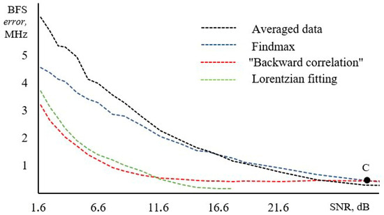
Figure 2.
Comparison of different methods for finding the maximum of the Brillouin gain spectra (BGS) for frequency scanning step 1 MHz: Absolute error in finding the frequency (MHz) versus the signal-to-noise ratio (SNR) of the original spectrum, dB. Data on Lorentzian fitting is taken from [18].
It can be seen from the obtained dependence that the assumption made earlier is true—in general, at low SNRs the correlation method gives a smaller error in determining the BFS. The intersection point C of the curves “FindMax” and “Backward correlation” in Figure 3 (28.8 dB) is appropriate to be referred to as “critical SNR”. The dependence of the “critical SNR” on the frequency scanning step is shown in Figure 3. When SNR is below critical line, “backward correlation” method provides better accuracy. It follows from Figure 3 that the smaller the scanning step, the larger the SNR range where the correlation method gives better results than FindMax.
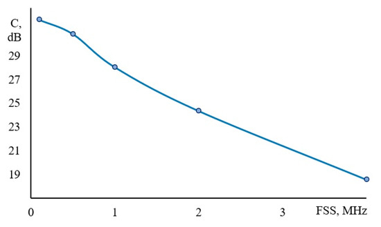
Figure 3.
Critical SNR C, dB versus frequency scanning step (FSS), MHz (obtained from simulation).
Thus, both assumptions about the range of applicability of the new method are confirmed by simulation results. The following is a description of the experimental part, where the proposed “backward correlation” method effectiveness was studied on the of application to real, not modeled data.
We tested our method with different spectral non-uniformities, obtained in the simulation as well—including the cases that significantly obstruct their comparison with the Lorentzian curve: High asymmetry of spectrum and “ghost” peaks. At first glance, the obtained results showed that the error in determining BFS does not depend significantly on the spectrum shape. We plan to study it in more details in future.
4. Experiment
For the experiment, we used a standard optical analyzer of the Brillouin spectrum in the time domain (BOTDA) DiTeSt STA-R-202 manufactured by Omnisens (Switzerland). As samples, optical fibers of the Panda-type were used. For the initial assessment, the following sensing mode was chosen—pulse duration 5 m; frequency scanning step (with automatic tuning of the system)—from 0.7 MHz to 5 MHz. The experimental results are presented at Figure 4.
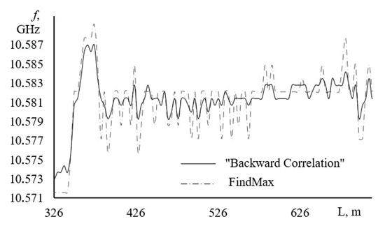
Figure 4.
Comparison of the results of the two methods on a real Brillouin optical time domain analyzers (BOTDA) trace.
In the course of the experiment, it was not possible to obtain the information of the exact values BFS along the length of the fiber in some other way; therefore, uniformity of the trace is proposed as the main criteria for the success of the application of both methods. The process of obtaining several kilometers of optical fiber from an up to half a meter preform in length almost eliminates the appearance of frequently repeated small inhomogeneities. Their presence on the trace can also be caused by winding the fiber onto the transport coil, but in the case of using a long (5 m) probe pulse, their appearance in the signal is practically excluded. Thus, uniformity assessment may be an adequate qualitative assessment of the effectiveness of the method. Both a visual inspection of the graphs and a comparison dispersion of values (9.7 × 10⁻⁴ for FindMax and 9.1 × 10⁻⁴ for the “backward correlation” method) indicate that with this SNR, the new method determines the BFS more accurately.
To test the efficiency of the method on a not so frequent, but no less actual task—measuring the distribution of birefringence (B) [19]—an experimental set-up was assembled based on the same DiTeSt STA-R-202. Two linear polarizers were connected with it. The fiber output of one of them was more than a kilometer long, which is required by the current BOTDA operation process. The polarizers are connected to the test sample (FUT) in such a way that linearly polarized radiation can be inputted from both sides into the FUT both at an angle of 0 degrees to the slow axis and 90 degrees of a Panda-type fiber. A probe signal is directed to the outer tip of the fiber, and pumping was inputted to the inner tip. The experimental set-up is shown at Figure 5.
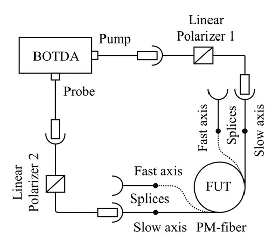
Figure 5.
An experimental set-up for obtaining the distribution of birefringence in a PM optical fiber.
This set-up allows one to obtain the spatial distribution of BFSs for each of the polarization states. Using them, to obtain modal birefringence, it is necessary to carry out a simple calculation [19]:
where nx and ny—the refractive indices of the slow and fast axis of the fiber at a certain point, respectively; λ—radiation wavelength; fx and fy—BFSs of the slow and fast axis at a certain fiber spatial point; and Vx and Vy—average speeds of sound in the slow and fast axis of the fiber. It should be noted that the use of exact values of Vx and Vy is an important condition for high-quality birefringence observation. These values were calculated using the core refractive index of the single-mode fiber, which is the output of one of the polarizers.
The same Panda-type fiber was used as a test sample. The parameters are given in the Table 1.

Table 1.
Fiber under test parameters.
A fiber with a length of about 1 km was wound in three layers on a typical corning transport coil of with a soft foam buffer, as shown in Figure 6. This was done in order to evaluate the performance of the method in close to real conditions, and the fiber was wound with the pressure of neighboring layers does not introduce significant distortions into the birefringence picture. The shades of gray in the figure at a qualitative level characterize the mechanical stress in each of the three layers of the coil.

Figure 6.
A schematic fragment of the studied fiber (FUT) cross-section on the transport coil.
Figure 7 shows two alternately measured polarization-BOTDA traces of the studied fiber. The red curve shows the data obtained by probing the sample with linearly polarized radiation introduced at 0 degrees to the slow axis of the fiber. The blue curve is the same, but at an angle of 90 degrees to the slow axis. It is seen that the longitudinal tension of the fiber monotonically increases from the outer end to the inner end—this can be caused by the winding process details. These details also explain two bursts after the first and second layer (the winding take-up unit makes an abrupt change in the move direction, and the mechanism that compensates for the tension does not have time to work). The transverse pressure under the conditions of uncontrolled axial torsion of the fiber acts on the polarization state [20], however, this did not affect the quality of the conducted experiment in this case.

Figure 7.
BOTDA-traces for slow and fast axes of the studied fiber (f, GHz versus length, m).
After processing with the use of expression (4) for the two compared methods, the length distribution of modal birefringence is shown in Figure 8. To begin with, it should be noted that the processed data do not contain those distinctive features of the source data, the effects of which were to be avoided: These are variations in the tension between the winding layers and the general trend are not remaining the same. Since the problem of obtaining the distribution of B along the length of the anisotropic optical fiber is quite demanding on the accuracy parameters of the measuring system, after processing by both compared methods, spatial accumulation of data was carried out in a sliding window of 10 samples. This made the obtained dependencies more visual.
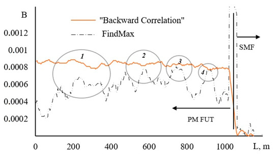
Figure 8.
Distribution of modal birefringence along the length of an anisotropic optical fiber. Marked by circles are the four regions where the birefringence changes for both methods have details which look alike.
From Figure 8 it is obvious that the birefringence obtained by the “backward correlation” method is on average 8 × 10⁻⁴, which coincides with the fiber passport, while the algorithm with finding the maximum shows errors of up to 30–40% of the total values amount. There are also four areas where two methods demonstrate similar patterns of birefringence changes; but there are even more fragments on the graph where the data diverge significantly—perhaps this is due both to local variations of the SNR on the spectra corresponding to different fiber coordinates, and to the appearance of significant artifacts on them, significantly changing the symmetry of the spectral components.
5. Discussion and Future Work
FindMax algorithm does not take into account the whole spectrum, it deals only with the very central part of it, that is why it gives that bad results at low SNR—every single statistical outlier leads to a significant error in determining BFS. Spectrum averaging effectively increases SNR, shifting the whole curve (see Figure 2) to the left but at the same time preserving its shape. It allows to expand the range of method applicability but does not save from catastrophic raise of error at low SNR (and at very low SNR could even lead to opposite result—error for finding maximum after preliminary spectrum averaging becomes even larger, see region of Figure 2 below 16.6 dB). The proposed method is not subject to this limitation, in this respect resembling the approach of spectrum reconstruction.
Another issue of FindMax algorithm is discretization. Even at infinite SNR the error in determining BFS could not be smaller than quarter of a frequency scanning step. Since the “Backward-correlation” operates only with spectra shifted by integer step, in this respect it is similar to FindMax. It makes proposed method not effective at high SNR where modern algorithms give an error much lower than frequency scanning step.
One more possible advantage of “backward-correlation” method is that it does not rely on the exact shape of the peak. For example, Lorentzian fitting lacks its efficiency at low pulse durations since spectrum shape is no longer Lorentzian-like.
Another important point when comparing different methods is their computational cost. “Backward-correlation” requires calculation of only N correlations where N is a number of samples in the spectrum. One does not have to cycle through all possible combinations of Lorentzian fit parameters.
At the same time, the proposed method has some systematic errors, as it was described above. Our results show that in spite of these systematic errors it still could give better results than FindMax algorithm. Of course, a new method has to be compared not only with FindMax, but also with other techniques, especially with Lorentzian fitting used by state-of-the-art BOTDA. Complete modelling of Lorentzian fitting algorithms is beyond the scope of this paper, but we can use the results presented in the references [12,18] for comparison. Error in determining BFS by Lorentzian fitting scales drastically at SNR < 5 dB and data from Figure 2 show that new method is quite comparable with Lorentzian fitting and even gives smaller error at these conditions. In more details the comparison of the new method with Lorentzian fitting must be studied in future.
As it has been already stated, the lower the SNR and the lower the frequency scanning step, the higher the potential benefit of the proposed method is. At frequency scanning steps less than 1 MHz, for example, the “backward correlation” method provides better accuracy almost independently from SNR. At higher frequency scanning steps, the range of method applicability is limited to low-SNR region, what can be of interest for low-cost real-time Brillouin sensors. According to the simulation (see Figure 2) and experimental data (see Figure 4), the error of BFS determination by processing of single not-averaged spectrum can be lowered by 1–2 MHz, which undoubtedly should be investigated as applied to distributed fiber optic sensors. The algorithm for calculating the typical correlation function has been successfully tested over the years in a wide range of reflectometry systems [21,22], so there is no doubt that with the changes made (the reverse movement of the second discrete function), it will work successfully and without delay in real time in commercial sensor systems. As for the practical success of the method, demonstrated at a qualitative level (including, in the case of calculating the distributed modal birefringence of an anisotropic optical fiber), it requires further comprehensive study and repetition on different measuring systems and samples. Although it has been previously shown that the influence of winding as an external factor is not so noticeable when studying the distribution of birefringence, in the future this may be the topic of a separate work, in which external factors, such as winding tension and the number of overlaps will be quantified.
Summary of different methods comparison is presented in Table 2.
Table 2.
A comparison of all discussed methods obtained from data simulated with the 1 MHz scanning step (SS).
6. Conclusions
We present a new, based on correlation analysis, method of finding Brillouin spectrum maximum. The developed method has demonstrated its advantages over the simplest way of calculating the maximum of the BGS—both on simulated spectra and on the data obtained in the experiment. The fact that the method is effective on real data with a high noise level most likely demonstrates its main role in the potential cheapening of Brillouin reflectometers and analyzers, where it becomes possible to use less expensive photodetectors. At the same time, it will be possible to get a benefit in reducing the time of data accumulation only in a number of cases—single, not averaged BGS do not always contain correct information about the position of the maximum, whatever SNR they may have.
Possible applications of the method in modern distributed optical sensors: Hardware/software improvement of typical fiber optic sensors and modal birefringence distributed study are discussed. The method could be useful for processing of ultralow SNR signals in BOTDR/BOTDA applications.
Author Contributions
Idea, development, computer experiment, programming, data processing—F.L.B. and Y.A.K.; experiment—A.I.K. All authors have read and agreed to the published version of the manuscript.
Funding
The work was performed as a part of state assignment No. AAAA-A19-119042590085-2.
Acknowledgments
The authors are grateful to PNPPK, PJSC (Perm Scientific and Industrial Instrument-Making Company, Perm, Russia) for their help in performing experiments.
Conflicts of Interest
The authors declare no conflict of interest.
References
- Hartog, A. An Introduction to Distributed Optical Fibre Sensors; CRC Press: Boca Raton, FL, USA, 2017. [Google Scholar] [CrossRef]
- Urricelqui, J.; Soto, M.; Thévenaz, L. Sources of noise in Brillouin optical time-domain analyzers. In Proceedings of the 24th International Conference on Optical Fibre Sensors, Curitiba, Brazil, 28 September 2015; Volume 9634. [Google Scholar] [CrossRef]
- Zheng, H.; Fang, Z.; Wang, Z.; Lu, B.; Cao, Y.; Ye, Q.; Qu, R.; Cai, H. Brillouin frequency shift of fiber distributed sensors extracted from noisy signals by quadratic fitting. Sensors 2018, 18, 409. [Google Scholar] [CrossRef] [PubMed]
- Zaslawski, S.; Yang, Z.; Soto, M.; Thévenaz, L. Impact of Fitting and Digital Filtering on Signal-to-Noise Ratio and Brillouin Frequency Shift Uncertainty of BOTDA Measurements; ThE27; Optical Society of America: Washington, DC, USA, 2018. [Google Scholar] [CrossRef]
- Soto, M.; Thévenaz, L. Modeling and evaluating the performance of Brillouin distributed optical fiber sensors. Opt. Express 2013, 21, 31347–31366. [Google Scholar] [CrossRef] [PubMed]
- Feng, C.; Preussler, S.; Kadum, J.; Schneider, T. Measurement accuracy enhancement via radio frequency filtering in distributed brillouin sensing. Sensors 2019, 19, 2878. [Google Scholar] [CrossRef] [PubMed]
- Gyger, F.; Yang, Z.; Soto, M.; Yang, F.; Tow, K.; Thévenaz, L. High Signal-to-Noise Ratio Stimulated Brillouin Scattering Gain Spectrum Measurement; ThE69; Optical Society of America: Washington, DC, USA, 2018. [Google Scholar] [CrossRef]
- Urricelqui, J.; Sagues, M.; Loayssa, A. Synthesis of Brillouin frequency shift profiles to compensate non-local effects and Brillouin induced noise in BOTDA sensors. Opt. Express 2014, 22. [Google Scholar] [CrossRef]
- Feng, Z.; Gan, J.; Lv, H.; Cui, L. Application of wavelet analysis in distributed optical fiber Brillouin temperature strain monitoring system. IOP conference series. Earth Environ. Sci. 2018, 189, 032026. [Google Scholar] [CrossRef]
- Zhang, Z.; Hu, W.; Yan, J.; Zhang, P. The research of optical fiber Brillouin spectrum denoising based on wavelet transform and neural network. Proc. SPIE Int. Soc. Opt. Eng. 2013, 8914, 891408. [Google Scholar] [CrossRef]
- Minardo, A.; Caccavale, M.; Coscetta, A.; Esposito, G.; Matano, F.; Sacchi, M.; Somma, R.; Zeni, G.; Zeni, L. Monitoring test of crack opening in volcanic tuff (Coroglio Cliff, Italy) using distributed optical fiber sensor. In Geophysics: Principles, Applications and Emerging Technologies; 2016; Available online: http://eprints.bice.rm.cnr.it/14412/1/978-1-63484-852-7_eBook_Geophysics.pdf (accessed on 21 September 2020).
- Feng, C.; Lu, X.; Preussler, S.; Schneider, T. Gain spectrum engineering in distributed brillouin fiber sensors. J. Lightw. Technol. 2019, 37, 5231–5237. [Google Scholar] [CrossRef]
- Jia, X.; Rao, Y.; Wang, Z.; Zhang, W.; Ran, Z.; Deng, K.; Yang, Z. Non-local effect in Brillouin optical time-domain analyzer based on Raman amplification. Qiangjiguang Yu Lizishu/High power laser and particle. Beams 2012, 24, 1667–1671. [Google Scholar] [CrossRef]
- Dragic, P.; Kucera, C.; Furtick, J.; Guerrier, J.; Hawkins, T.; Ballato, J. brillouin spectroscopy of a novel baria-doped silica glass optical fiber. Opt. Express 2013, 21, 10924–10941. [Google Scholar] [CrossRef] [PubMed]
- Barkov, F.L.; Yu, A.; Konstantinov, V.; Burdin, V.; Krivosheev, A.I. Theoretical and experimental estimation of the accuracy in simultaneous distributed measurements of temperatures and strains in anisotropic optical fibers using polarization-brillouin reflectometry. Instrum. Exp. Tech. 2020, 20. [Google Scholar] [CrossRef]
- Konstantinov, Y.; Kryukov, I.; Pervadchuk, V.; Toroshin, A. Polarisation reflectometry of anisotropic optical fibres. Quantum Electron. 2009, 39, 1068–1070. [Google Scholar] [CrossRef]
- Thévenaz, L.; Nikles, M.; Robert, P. High-accuracy Brillouin gain spectrum measurements of single mode fibers. In Proceedings of the Symposium on Optical Fiber Measurements, Boulder, CO, USA, 1 January 1994; pp. 211–214. Available online: https://www.researchgate.net/publication/259670553_High-accuracy_Brillouin_gain_spectrum_measurements_of_single_mode_fibers (accessed on 21 September 2020).
- Haneef, S.; Yang, Z.; Thévenaz, L.; Venkitesh, D.; Srinivasan, B. Performance analysis of frequency shift estimation techniques in Brillouin distributed fiber sensors. Opt. Express 2018, 26, 14661. [Google Scholar] [CrossRef] [PubMed]
- Smirnov, A.; Burdin, V.; Konstantinov, Y.; Petukhov, A.; Drozdov, I.; Kuz’minykh, Y.; Besprozvannykh, V. Birefringence in anisotropic optical fibres studied by polarised light Brillouin reflectometry. Quantum Electron. 2015, 45, 66–68. [Google Scholar] [CrossRef]
- Barkov, F.L.; Konstantinov, Y.A.; Bochkova, S.D.; Smirnov, A.S.; Burdin, V.; Krivosheev, A.; Nosova, E.A.; Smetannikov, O.Y. Modelling of polarised optical frequency domain reflectometry of axially twisted anisotropic optical fibres. Quantum Electron. 2019, 49, 514–517. [Google Scholar] [CrossRef]
- Kwon, Y.-S.; Seo, D.-C.; Choi, B.-H.; Jeon, M.Y.; Kwon, I.-B. Strain measurement distributed on a ground anchor bearing plate by fiber optic OFDR sensor. Appl. Sci. 2018, 8, 2051. [Google Scholar] [CrossRef]
- Froggatt, M.; Gifford, D.; Kreger, S.; Wolfe, M.; Soller, B. Distributed strain and temperature discrimination in unaltered polarization maintaining fiber. Optics Fiber Sens. 2006. [Google Scholar] [CrossRef]


© 2020 by the authors. Licensee MDPI, Basel, Switzerland. This article is an open access article distributed under the terms and conditions of the Creative Commons Attribution (CC BY) license (http://creativecommons.org/licenses/by/4.0/).