1. Introduction
Over time, the acoustic characteristics of rooms have assumed considerable importance in many areas of people’s personal and working life. Being able to have an undisturbed conversation in a restaurant or a pub, listen to an orchestra concert in a room with adequate sound distribution and diffusion, as well as study and teach in quiet classrooms with excellent intelligibility of the speaker are all examples of how the correct acoustic design of spaces can influence our experience of daily life. The parameters that most influence our perception of the acoustic quality of a living, working, or playful environment are, for example, the background noise, reverberation time, and homogeneity of the sound distribution. Among these, the control of reverberation in the rooms is certainly of fundamental importance. Systems suitable for reducing reverberation times in environments exploit the geometric characteristics and porosity of the materials they are made of to increase sound absorption, and therefore, reduce overall sound pressure levels [
1,
2].
The use of sound absorbers within an environment affects the propagation of sound from a source, and therefore, the sound pressure levels distributed in the environment. In a conference room, listeners in the stalls can perceive a speaker’s speech adequately if the characteristics of the interior surfaces of the environment have been designed to propagate sound effectively. An environment that is too reverberating will produce high levels of sound pressure, but at the expense of intelligibility, while an environment that is too absorbing could result in insufficient sound pressure levels for a good understanding of speech. The installation of sound-absorbing false ceilings and wall coverings, capable of appropriately attenuating the reflection of incident sound waves, is a type of environmental acoustic correction that has been widely used and tested for decades, with which the reverberation time can be brought to optimal values. Sound absorbing materials reduce the acoustic energy of a sound wave as it passes through the material. For the absorbent material to function properly, it must be porous or fibrous. The acoustic wave that propagates in the material loses energy by viscous dissipation. The fibers are also excited to collide with each other, producing heat that leads to further dissipation of acoustic energy. A fundamental requirement for the sound-absorbing layer is that the surface that receives the incident sound wave must be poorly reflective, allowing the passage of sound within the material. All the power is reflected and in fact destined to return to the system in another form. It is therefore clear how a good sound absorbing will certainly be a barrier of poor effectiveness [
3,
4,
5,
6].
The acoustic correction of spacious environments is often extremely problematic, and for these large spaces, it is necessary to correct the components of the sound tail present in the medium and low frequencies. What is added to all this are aesthetic constraints that, for some places such as ancient churches or historic buildings, represent an obstacle that puts the designer in serious difficulty. In fact, in these places, it is not possible to think of corrective solutions that make use of traditional panels of sound-absorbing material to be applied to the walls: This is due to aesthetic, historical, or architectural reasons. In these cases, it is necessary to hypothesize alternative solutions that allow us to carry out the acoustic correction of these places. A solution must necessarily address design solutions that involve the use of materials with a pleasant appearance [
7,
8].
A product often used for the cladding of prestigious buildings is ceramic material: Ceramic materials are inorganic nonmetallic materials, consisting of metallic and nonmetallic elements linked together mainly by ionic and/or covalent bonds. The chemical compositions vary considerably: From simple compounds to mixtures consisting of many complex phases linked together. Usually, to indicate a porous ceramic material, made with crystalline paste and without coatings, the term “terracotta” is adopted. Today, terracotta is largely represented by ceramic products intended for use in building constructions, which are commonly classified under the name of bricks [
9]. Among the salient features of a brick, the modularity of the shape stands out, and therefore, the possibility of creating a standardized and easily replicable product; durability over time and good resistance to atmospheric agents; and a low thermal conductivity and a relatively low cost. From ancient times until the nineteenth century, the production techniques of bricks consisted mostly of processes that included an exclusively manual molding, drying carried out naturally by exposure to the heat of the sun, and firing in ovens with the temperature and degree of oxidation strongly inhomogeneous from zone to zone. Thanks to the advent of driving machines and the first production rationalization systems, it was possible to make the forming operation completely mechanical. Furthermore, the enriched knowledge derived from the studies of thermodynamics and gas motions has allowed the construction of ovens capable of preheating the dry material thanks to the smoke draft devices controlling the supply of fuel and combustion air necessary to cooking. These technological advances have therefore made it possible to raise the quality and production quantity of bricks [
10,
11].
Helmholtz resonators are special acoustic resonant cavities created by Hermann von Helmholtz in 1860 for the study of sound and its perception. They can simply be constructed as metal vessels, usually spherical or cylindrical, of various sizes with a narrow opening preceded by a short, narrow neck. It is known that by blowing air through the neck of an empty bottle, a sound can be heard: The bottle acts as a resonator [
12,
13]. Large ceramic or bronze vases, jars, and smooth stone cavities with large openings exposed to sound seem to have been used in ancient theaters to amplify the voice of the actors and are mentioned in the treatise De Architectura by Vitruvius [
14], a Roman architect who lived in the 1st century BC. Later, these simple resonators were called Helmholtz resonators, named after the German scholar who first described their physical characteristics. These structures consist of a volume, containing air, connected to the cavity through a narrow neck and an opening. The energy of the incident sound causes the air contained in the neck of the resonator to vibrate, which due to its volume, behaves like a mass connected to a spring: In short, it is a sort of sound trap capable, depending on the conditions, to return or absorb energy. The empty cavity will therefore resonate at a specific frequency determined by the volume and size of the neck and the opening of the resonator [
15]. If the opening is wide and the cavity is empty, we speak of an active resonator because the system amplifies the sound that hits it, as indeed happens in any rigid and reflective cavity: Let us imagine an empty room with the door open, a vase in ceramic, etc. However, if we place sound-absorbing material inside the cavity, the system traps the sound that is dampened by the fibrous material, extending the absorption also to the adjacent frequencies. In this case, we are talking about a reactive resonator, that is, sound-absorbing [
16].
Finally, the possible applications of sound-absorbing materials made with ceramic can be varied. The need to use ceramic can derive from aesthetic or architectural needs; in fact, colored and glazed ceramic takes on a pleasant appearance that can easily be integrated into environments characterized by architectural constraints. Its use can be imposed by functional needs; in fact, it is a fireproof material, which can therefore be used in environments where high temperatures are reached, or in environments with a high risk of fire. Furthermore, these materials can be used to build sound-absorbing acoustic barriers, given its high resistance to shocks, as well as to light, climatic conditions, humidity, and chemical agents. Finally, these materials can be used for the acoustic correction of environments characterized by low-frequency sounds such as in churches, where traditional porous sound-absorbing materials are ineffective: The use of resonant surfaces can contribute to the reduction of unwanted low-frequency components.
This study reports the results of experimental measurements of the sound absorption coefficient performed on samples of ceramic material, made in an artisanal way. Sound absorption is obtained by appropriately drilling the discs of ceramic material. Specimens with hole sizes of 2 and 5 mm, and thicknesses of 3.0, 2.0, and 0.6 cm were made. The sound absorption of perforated sheets is based on the principle of Helmholtz resonators, which however, are effective only on narrow frequency bands; therefore, to make the phenomenon of absorption more effective and broaden the absorption frequency range, perforated panels are made, mounted at a certain distance from a rigid surface behind. The measurements of the sound absorption coefficient at normal incidence were performed with an impedance tube (Kundt tube) with an internal diameter of 10 cm and a length of 56 cm; the validity range of the measurement of the sound absorption coefficient is 100 Hz–2 kHz. Measurements of the absorption coefficient were performed, for each specimen, by creating an air cavity between the specimen and the rigid surface behind it. The measurements obtained were subsequently used to develop a numerical simulation model based on an artificial neural network algorithm.
2. Materials and Methods
Traditional ceramic materials are obtained by firing clayey minerals that contain inert and melting substances. They are classified according to the microstructure defined by porosity, the color of the support, and the surface coating. They are divided into porous paste products, consisting of grains separated by many pores and interstices, and compact paste products, in which the particles are welded together following the partial melting suffered during cooking [
17,
18]. The porosity of a ceramic product is fundamental in determining the mechanical characteristics and behavior in operating and environmental conditions. For example, a greater porosity corresponds to a worsening of the mechanical and frost resistance, but also an improvement in the thermal and acoustic insulation characteristics. Porosity is often assessed through the absorption of water. Conventionally, porous paste products are defined as having a water absorption higher than 5% [
19,
20].
2.1. Specimen Configuration
The name clay indicates a family of very heterogeneous sedimentary rocks, in which the minerals present in it perform the important plasticizing function, while the other components have a thinning and melting function. The clays are predominantly made up from hydrated aluminum silicates with a layered reticular structure, the general formula of which is: aAl
2O
3 ∙ bSiO
2 ∙ cH
2O. In addition to hydrated silicates, the clays also contain hydrated oxides, such as hydrated silica (SiO
2 ∙ nH
2O), hydrated alumina (Al
2O
3 ∙ nH
2O), and hydrated ferric oxide (Fe
2O
3 ∙ nH
2O). The hydrated aluminum silicates and, in part, the hydrated oxides are responsible for the plasticity of the clayey mixtures, that is, their ability to be modeled [
21].
There is also an inert part, consisting mainly of: Crystalline silica (quartz, quartzites, and siliceous sands), feldspar (potassium silico aluminates) and calcium carbonate (limestone). These constituents perform two important actions:
Leaning action by the siliceous sands which, having particles considerably larger than hydrated aluminum silicates, allow the regulation of the shrinkage during drying and cooking, also favoring the stability of the raw material after forming
Melting action of calcium carbonate. During the firing of ceramic materials, a liquid phase must be formed; this, upon cooling, solidifies, forming a compact glass that binds the grains of the material and fills the pores together. Calcium carbonate leads to the formation of a liquid phase at 950–1000 °C and is used as a flux for porous products obtained at low temperatures.
The clays are generally divided into fatty ones, that is, with a prevalence of clayey constituents, or lean, with a prevalence of inert constituents [
22]. If the clay is too greasy, it is necessary to add lean substances. The main feature of clay is plasticity, understood as the ability to deform under the action of external pressure and to retain the shape achieved even after the removal of this mechanical action. Plasticity is acquired in the presence of water in appropriate proportions and is lost after drying. The amount of water needed to give a clay plasticity depends mainly on its mineralogical structure and granulometry. In fact, the minute particles of hydrated silicates must be surrounded by a film of water thick enough to form a viscous coating, capable of allowing their reciprocal movement. In addition, the water adheres to the surface of the crystals, allowing the shape imparted to the product to be preserved, even after the removal of external stress. Plasticity increases with water content until the mixture becomes fluid. A greater plasticity corresponds to a simpler shaping of the products, but also increases the shrinkage during drying due to the removal of the film of water that is between the particles. The latter, if excessive, can give rise to deformations and tensile stresses capable of compromising the integrity of the products. Plasticity is gradually lost during drying, following the removal of the mixing water [
23]. During firing, then, the loss of plasticity tends to be less and less recoverable, until it is completely lost at about 600–700 °C, when there is the decomposition of hydrated silicates.
The preparation of the specimens was performed through the following steps:
Preparation of the dough. The raw materials are ground and mixed, and the resulting mixture is homogenized. The ground products are first sieved and then dry-mixed according to suitable weight or volume ratios. The dry process is applied to products obtained from a single raw material.
Forming. By forming, the dough is given the shape of the desired product with the application of sufficient pressure to deform it plastically and stably. After forming, the blank must be strong enough to withstand its own weight and stresses during handling.
Drying. The water contained in the raw must be removed before cooking by means of a delicate drying process, with which the water that forms a veil around the clay particles is removed, giving plasticity to the material. During this process, there is a contraction in volume due to a rapprochement of the particles with an increase in the mutual forces of attraction and, therefore, in the mechanical strength of the product. Artificial drying begins in a very humid environment (relative humidity = 70%, and temperature = 50 °C), where the product is heated without loss of water, favoring the water flow from the inside to the surface. The humidity is then gradually decreased, and the temperature increased, without exceeding 120 °C. Subsequently, the water contained in the internal pores of the clay particles is also removed, but this process is not associated with any contraction of the dough. The drying continues until the moisture content of the product is not less than 1%.
Cooking. Through cooking, the dried doughs acquire their final physical-mechanical properties, dimensions, and appearance. The firing process with variable temperature between 900 °C and 1000 °C must be homogeneous to create a material with adequate porosity. During cooking, the clay disintegrates, releasing its oxides, namely silica (SiO
2) and alumina (Al
2O
3). Above 900 °C, the limestone decarbonates and the formation of a compound between alumina and silica called “mullite” (3Al
2O
3 ∙ 2SiO
2) begin; in this phase, there is also the gradual formation of a liquid phase that fills the voids between the particles [
24].
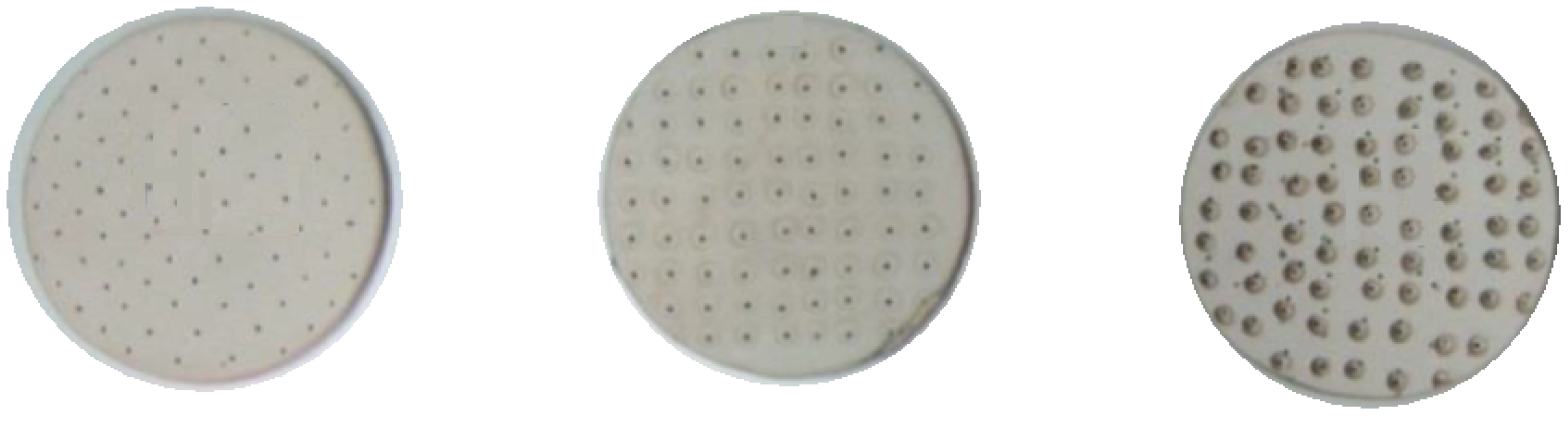
To measure the sound absorption properties, specimens were made with different thicknesses but with a diameter of 10.0 cm. In this way, the specimens are compatible with the dimensions of the internal diameter of the specimen holder of the impedance tube that will be used for the measurements. In the initial phase, which involves mixing the clay and modeling the specimen, the dimensions of the specimens are larger than those of the finished product. This is due to the presence of the water necessary for modeling the specimen. The thicknesses of the specimens provided are: 0.6, 2.0, 2.5, and 3.0 cm. The clay is initially a plastic material, easily modeled, but during the making of the specimens, it was difficult to obtain the circular shape. To solve the problem, during drying, the shape of the specimen was maintained using cardboard strips placed on the perimeter of the same. Subsequently, the discs were drilled, which was made with the aid of a square sheet of cork on which a regular grid of points was drawn in correspondence with which headless nails were inserted. The specimens were then made by spreading a piece of clay on the cork sheet fitted with nails. A pressure on the specimen itself was carried out to make the holes at a regular pitch, then with the aid of an awl, the holes were finished (
Figure 1).
We then moved on to the drying phase; after a few days of air drying, the pieces lost their humidity and plasticity and the preset shape was fixed. After the drying phase, which lasted about five days, the edges of the circular-section specimens were finished, making them as smooth as possible by sandblasting, to facilitate housing in the specimen holder. Finally, cooking was carried out in special ovens at a temperature of about 1000 °C. Firing is a process that lasts many hours and is a very delicate phase, as sudden changes in temperature can cause the piece to break. The thinner specimen (0.6 cm) created some problems as it was slightly deformed due to shrinkage due to water loss.
2.2. Helmholtz Resonator-Based Setup
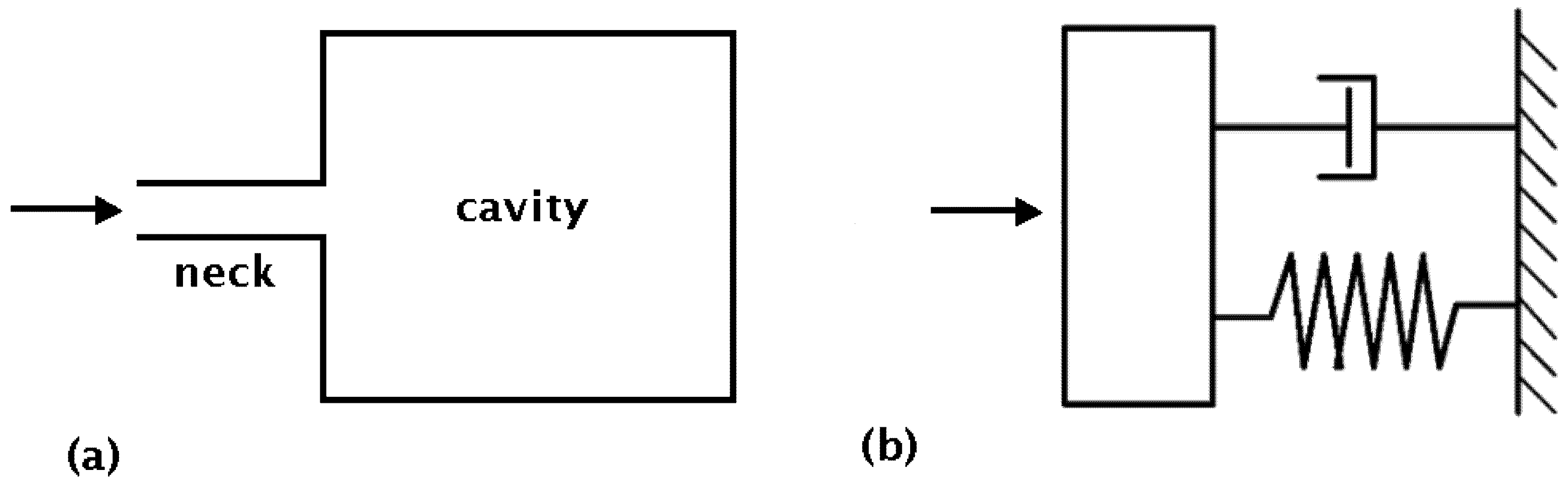
Helmholtz resonators are formed by a cavity placed in communication with the environment by means of a small hole, called the resonator neck, of generally negligible dimensions compared to those of the cavity [
25]. When a sound wave affects the resonator inlet, the air contained in the neck is placed in oscillation, behaving like an oscillating piston, while the air contained inside the cavity is alternately compressed and expanded acting like a spring (
Figure 2).
This system consisting of an oscillating mass given by the air in the resonator neck, an elastic element (air in the cavity), and a damping element due to the friction on the neck walls will have its own resonance frequency at the maximum vibration, which will be the maximum dissipation of sound energy. The absorption of the resonators is high at the resonant frequency but very low for all the other frequencies. It is thus possible to build calibrated devices to absorb specific frequencies [
26]. In the technique, it is also used to fill part or all the cavity with porous absorbent material, or this material is added only at the neck. These changes broaden the spectrum of operating frequencies, decreasing the effect at the resonant frequency, however. Currently, rigid perforated panels are used, fixed at a certain distance from the wall. The acoustic behavior of these panels is like that of a classical resonator, even if they are less efficient. In this case, filling the cavity with porous materials effectively improves the frequency behavior of the structure [
27]. The optimal absorption field is centered on the medium frequencies. For the construction of these panels, different materials are used, such as metal materials, plaster, wood, or plastic materials [
28].
In this study, to measure the acoustic properties of the material under examination, the specimens in ceramic material were housed inside the impedance tube, leaving a cavity of 5 cm to simulate the Helmholtz resonator behavior.
2.3. Impedence Tube Measurements
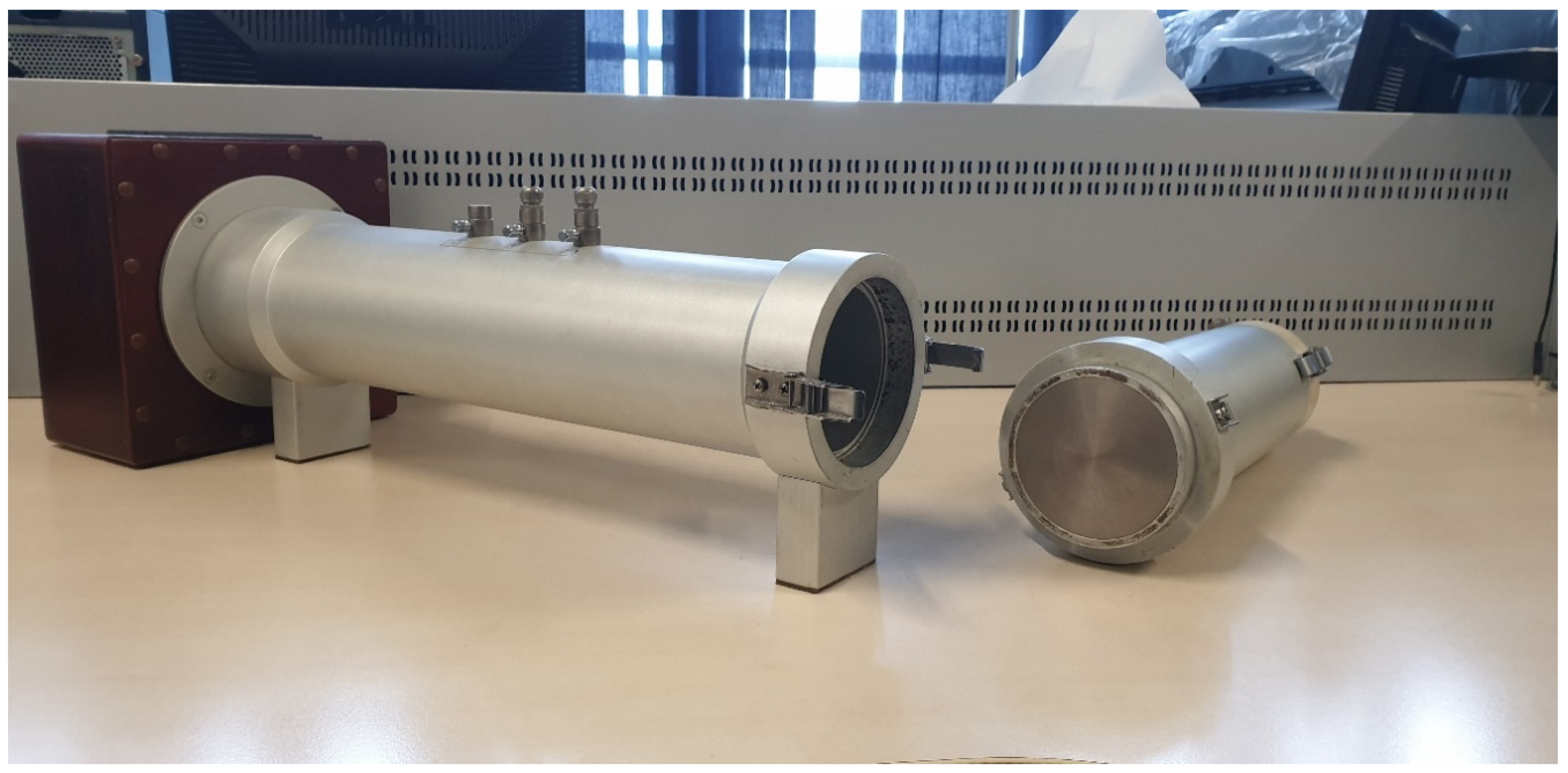
For the measurement of the normal incidence sound absorption coefficient, an impedance tube made in accordance with the UNI EN ISO 10534 2 ISO: Geneva, Switzerland [
29] standard was used. The measuring tube has the following dimensions: Internal diameter of 100 mm, length 560 mm, and distance between the two microphones equal to 50 mm (
Figure 3).
Due to the size of the tube, the internal diameter, and the distance between the two measurement microphones, the normal incidence absorption coefficient value is applicable in the frequency range between 100 Hz and 2.0 kHz.
2.4. Artificial Neural Network-Based Model
Artificial neural networks (ANNs) are a family of machine learning techniques composed of layers of interconnected neurons, with an architecture like that of biological neurons [
30]. The development of neural networks takes inspiration from biology, as the functioning of artificial networks mirrors that of the brain, based on several interconnected neurons working in parallel, which process an input, producing an output that will be sent to subsequent neurons. The biological neuron is formed by a central body, called somas, in which we have the nucleus; connected to it are the dendrites, which receive signals from other nearby neurons and transport it to the cell body, and the axon, which conducts the output signal in the direction of other surrounding cells. These two neurites differ, in addition to the task performed, in shape: The dendrites are thinned from the initial to the terminal part and are not good conductors, by decreasing the intensity of the signals, while the axon has a constant section and, being enveloped by myelin, turns out to be an excellent conductor. The neuron is characterized by two possible states: An active state, during which signals are passed, and a rest state, in which the neurons are polarized and a difference in charge occurs between the inside and the outside, and there is no passage of information through the neurites [
31].
In a biological neuron, therefore, the input is composed of a combination of signals that reach it through the numerous connected dendrites; the input signals can be both excitatory and inhibitory, resulting in a different value to be attributed to each of them. The combination of the input signals, if the threshold value is exceeded, establishes the activation of the neuron, letting the processed signals flow through the axon; otherwise, the neuron does not activate, and the signal is not transmitted. A very interesting aspect of the functioning of the brain is its ability to continuously vary the weights of the interconnections, making it possible to classify and generalize the stimuli received from the outside, favoring adaptation by learning from past signals and consequently training to facilitate learning, allowing new data to be processed more quickly and correctly [
32].
Artificial neural networks (ANN) are based on the functioning of the animal brain, defining the central body as a mathematical model, called a node, characterized by an activation function, a threshold value, and possibly a bias. Each node receives as input a set of signals (x) from the previous units. These signals reach the neuron after being weighed and their combination, after having algebraically summed the bias if present, becomes the variable of the activation function, resulting in the activation, or nonactivation, of the neuron [
33].
Let us consider
x = (
x1, …,
xn) as a set of independent variables, defined as network inputs, and
y = (
y1, …,
yk) as a set of dependent variables, which represents the network output. Then, consider
w = (
w1, …,
wn) as a set of weights. The association between output and input of the network can be exemplified through the following equation:
In Equation (1):
The choice of the activation function determines the substantial difference with the corresponding biological neuron. In the latter, the sum of the incoming impulses is transmitted directly to the axons if the threshold is exceeded, essentially behaving like a linear regression model, approximating the distribution of data with a straight line, while the use of a nonlinear function allows, instead, to have a better representation of the signals, without considering that, sometimes, a linear regression is not usable [
34].
A neural network is, therefore, a set of nodes arranged in layers, called layers, linked together by weights. The first layer is called the input layer, the last is the output layer, while the intermediate ones are defined as hidden layers and are not accessible from the outside, as all the characteristics of the complete network are stored in the matrices that define the weights (
Figure 4).
The type of network determines the type of connections that are present between the nodes of different layers and between those of the same layer. For ease of understanding, the typical feedforward configuration will be used to illustrate the characteristic elements of neural networks, in which each node is connected to those of the previous layer, from which it receives inputs, and to those of the next layer, to which it provides output [
35].
3. Results
To characterize the acoustic behavior of the ceramic resonators, seven specimens of different thicknesses, diameters of the holes, and percentages of perforation were made. In this way, seven different types of specimens were made with four different thicknesses, four different hole diameters, and many different percentages of perforation.
Table 1 shows the characteristics of the specimens subjected to measurement.
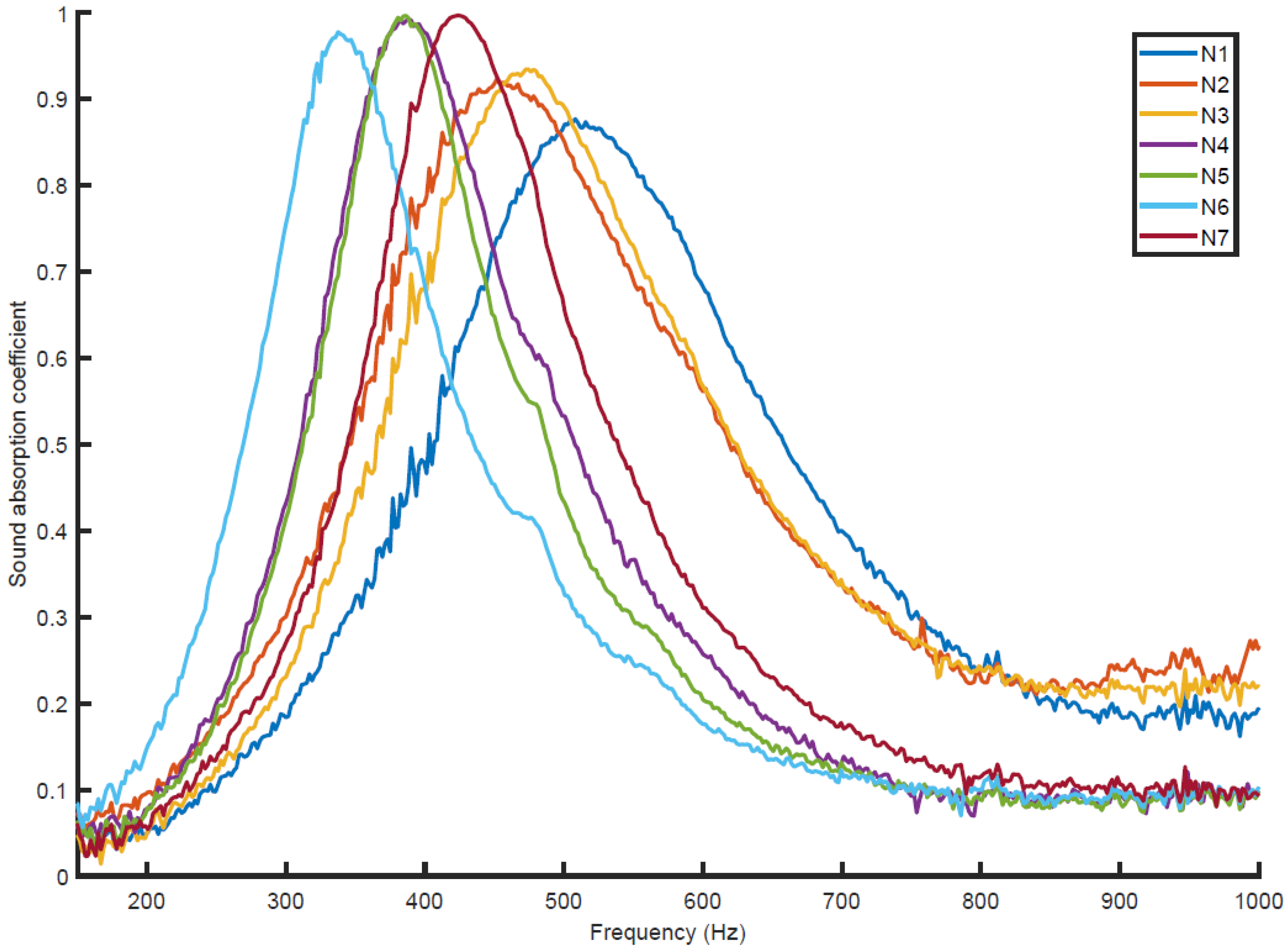
Figure 5 shows the values of the sound absorption coefficient measured at normal incidence as a function of frequency, for each of the seven types of specimen identified by the ID as shown in
Table 1. The cavity thickness is 5 cm, while the values of the absorption coefficients are reported in frequency function, and for greater ease of understanding, they are reported in the frequency range from 150 Hz to 1.0 kHz. First, we can note that the trends of the sound absorption coefficient as a function of frequency take on the characteristic shape of a bell curve typical of porous materials. We then analyze the results as a function of the specimen specifications to understand how they characterize their behavior. We begin with the analysis of the contribution of the thickness of the specimen on the trend of the sound absorption coefficient. We remind you that the specimens are characterized into four different thicknesses (0.6, 2.0, 2.5, and 3.0 cm). We can see that as the thickness of the specimen increases, the peak of the bell curve shifts toward lower frequencies, going from just over 500 Hz to about 350 Hz.
Furthermore, we can note that the greater thicknesses have a higher peak value of the sound absorption coefficient, almost reaching the maximum value. However, for the greater thicknesses, we can notice that the bell curve narrows; in this case, the frequency range that gives interesting values of the sound absorption coefficient is shortened. In fact, for the thickness of 0.6 cm of specimen N1, we can read a value of the sound absorption coefficient greater than 0.5 for frequency values ranging from 400 to 700 Hz. If we analyze the curve relating to the thickness of 3.0 cm of specimen N7, we note that values of the sound absorption coefficient greater than 0.5 are obtained for frequency values ranging from 350 Hz to just over 500 Hz.
Let us analyze the contribution provided by the diameter of the holes made on the specimen. For example, let us investigate the N2 and N3 specimens characterized by the same thickness equal to 0.6 cm but with different hole diameters and respectively equal to 0.3 and 0.6 cm. In this case, we can see that the increase in the diameter of the holes determines a shift in the peak of the bell curve toward higher frequencies. The same thing occurs if we compare the N6 and N7 specimens characterized by the same thickness equal to 2.5 cm but differentiated by hole diameters equal to 0.3 and 0.6 cm, respectively. In addition, in this case, an increase in the diameter of the holes determines a shift in the curve towards higher frequencies. All this is consistent with the performance returned by a Helmholtz resonator, which offers a very selective sound absorption around its resonance frequency, which is directly proportional to the section of the neck (in our case, with the diameter of the holes), and inversely proportional to the length of the neck (in our case, the thickness of the specimen).
To simulate the acoustic behavior of the ceramic material, a model based on artificial neural networks was developed. The data obtained from the measurements of the sound absorption coefficient carried out with the use of the impedance tube were used as input together with the geometric characteristics of the specimens. A dataset was built containing the following fields:
Then, 3368 records were collected containing the values of the sound absorption coefficient in correspondence with the frequency values, thickness of the specimen, and diameter of the holes. The first three fields of the database were used as input, while the last field, that is, the sound absorption coefficient, was used as output.
Normally, to generalize correctly in an automated way, the database is fragmented through a cross-validation in two parts: A training part and a test part. A common fragmentation procedure adopted by the scientific community is cross-validation [
36]. It is a statistical technique used in machine learning to eliminate the overfitting problem in the training set. When performing
k-times cross-validation, the original sample is split into
k subsamples of the same size. Of these
k subsamples, one is stored as validation data to test the model and the remaining
k − 1 subsamples are used for training [
37]. This process is then repeated
k times and each
k subsample is used exactly once as validation data. Finally, the
k results from the
k repetitions of the process are combined by averaging to produce a single estimate. In this work, the K-fold cross-validation with
k = 5 was adopted [
38].
The crucial concept on which it is based is that of not using the entire set of data during the training of a model: Some of them are removed before the start of training. After the training is complete, the removed data can be used to test the performance of the learned model on new data. In other words, model validation is defined by the process in which a trained model is evaluated against a test dataset. The test dataset is a separate part of the same dataset from which the training set is derived. The main purpose of using the test dataset is to test the generalization ability of a trained model. Ultimately, the model is only evaluated after it has been trained. Along with model training, cross-validation aims to find an optimal model with the best performance [
39]. In this work, the training set was built using 70% of the records collected, and the test set was built using the remaining 30% of the whole dataset.
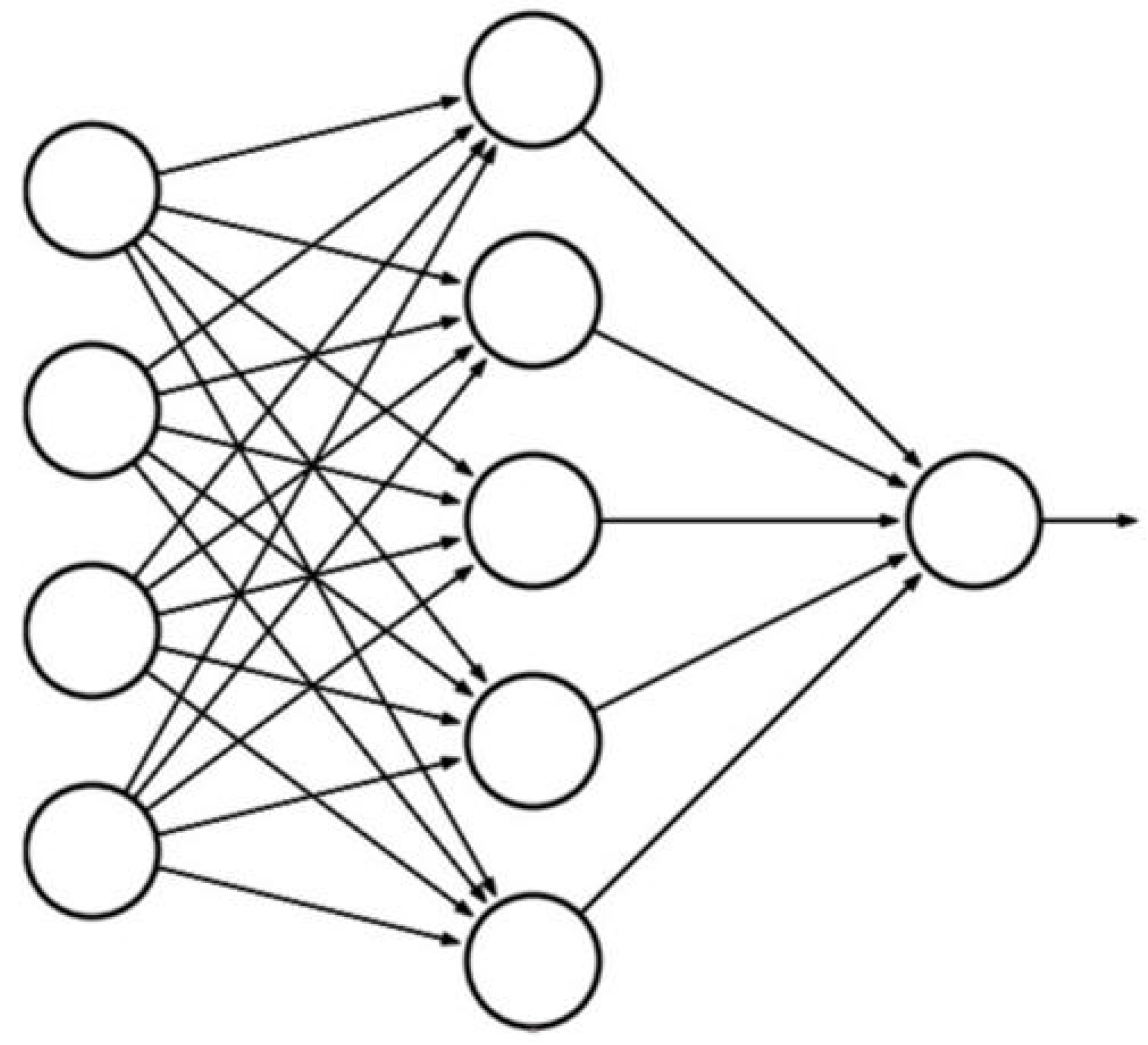
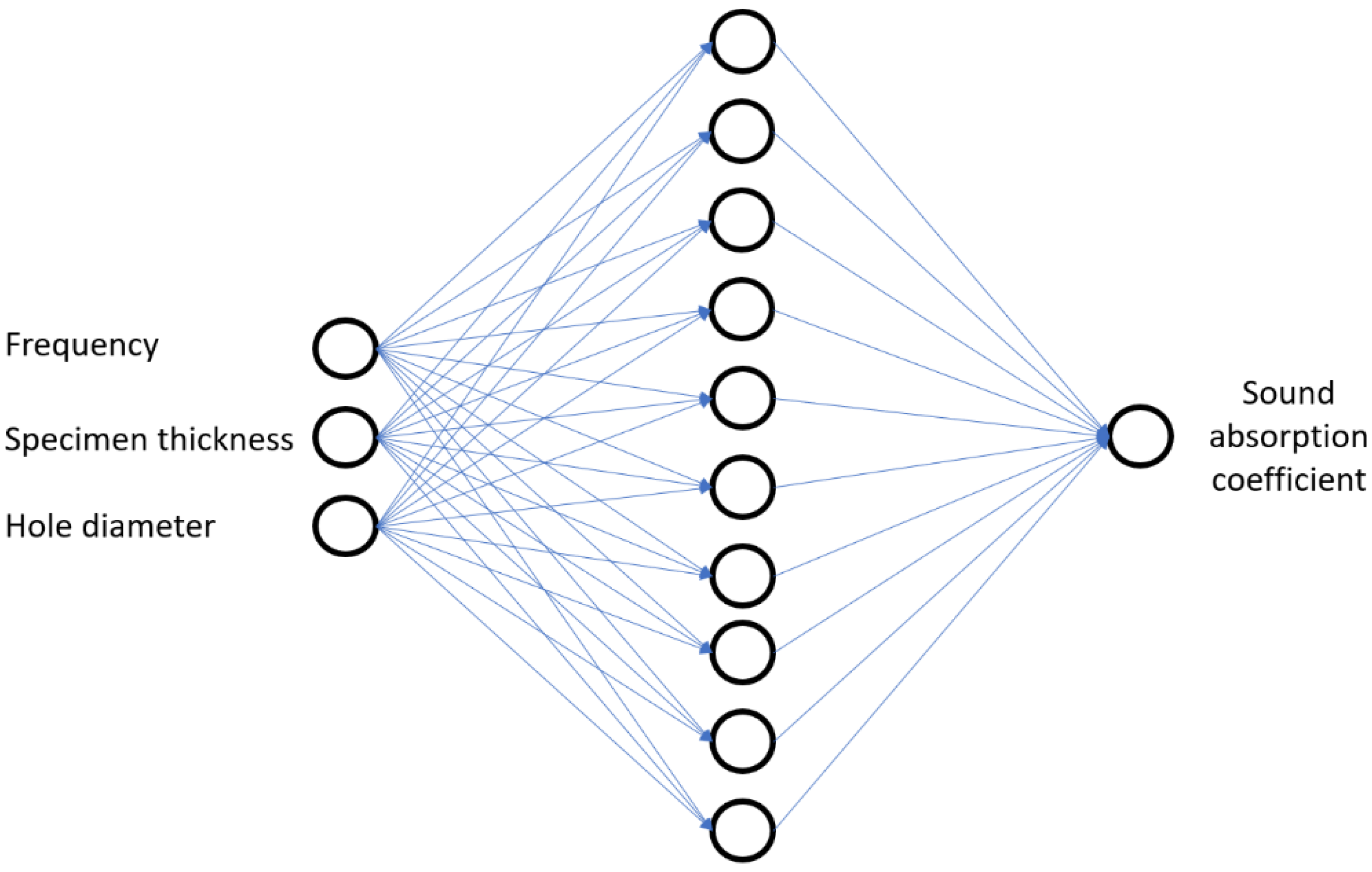
Figure 6 shows the architecture of the algorithm based on artificial neural networks used to simulate the acoustic behavior of a ceramic resonator.
Figure 6 shows a feedforward network architecture with an input layer, a hidden layer, and an output layer. Feedforward networks are those with the simplest architecture, being composed of an input layer, one or more hidden layers, and an output layer; each neuron has its input parameters from the previous layer and no cross-connections are possible between nodes of the same layer or cycles in which the output is sent to previous layers: The flow of information then proceeds in one direction only and, of each cycle, is determined only by the current input. Being a very simple type of network, it is by far the most used [
40,
41].
The training of a neural network consists of determining the values of the weights of the connections between all nodes and any bias, to map as accurately as possible the relationships that exist between inputs and outputs. The backpropagation technique was used to train the network. The final layer of the neural network has a neuron, and the value it returns is a continuous numeric value. The activation function adopted is the ReLu, which returns a numerical value greater than 0 [
42].
Backpropagation is based on two phases: The forward phase in which the network is crossed, and the error at the output is evaluated as the difference between the correct output and the one to be obtained; and the backward phase, that is, the back propagation itself, in which the signal propagates in the opposite direction and the weights are adjusted to reduce the output error. Back-propagation therefore adjusts the parameters of the neural network in the direction of the least error and is usually based on the application of the gradient descent method, which guarantees the finding of the local minimum of the cost function, indicating the direction of variation of the error to follow. It is also possible to find a global minimum by repeatedly searching for local minima and comparing them with each other. Based on the minimization of a cost function, the gradient descent training technique varies according to the type of problem to be studied and the error generated, on which the function chosen to be minimized directly depends [
43].
The Levenberg–Marquardt algorithm (LMA) was used to update the weights. It is an optimization algorithm used for the solution of problems in the form of nonlinear least squares, which commonly finds applications in curve fitting problems [
44]. LMA is an iterative algorithm, in which the update vector of the solution at each iteration is given by an interpolation between the Gauss–Newton algorithm and the gradient descent method. The LMA can be considered a trust region version of the Gauss–Newton algorithm, with respect to which it is more robust but, in general, slightly slower.
The following two metrics were used to evaluate the performance of the simulation model: Regression
R values and mean squared error. Regression
R values measure the correlation between outputs and targets. An
R value of 1 means a close relationship, and 0 a random relationship. Mean squared error (MSE) is the average squared difference between outputs and targets. Lower values are better. Zero means no error.
Table 2 shows the results of the simulated sound absorption coefficient of the ceramic resonator.
Figure 7 shows a comparison between the trend of the sound absorption coefficient as a function of frequency between the measurements carried out with the impedance tube and the simulations carried out with the model based on artificial neural networks.
The analysis of
Figure 7 confirms the results returned by the evaluation metrics adopted for the performance estimation. We can see that the simulated curves fit those returned by the measurements with the impedance tube. First, the typical bell curve characteristic of porous materials is confirmed; moreover, for each configuration of the specimen, a trend of the sound absorption coefficient is confirmed, which is distributed selectively around the resonant frequency of the resonator. Except for minor differences, the frequency for which the peak value is returned is confirmed, even if the simulation model seems to slightly undersize that value. The queue trends are also confirmed by showing a softening of the slopes presumably due to the optimization effect operated by the algorithms used in the model training phase.
4. Discussion
This work reports the results of experimental measurements of the sound absorption coefficient of ceramic materials using the principle of acoustic resonators. Subsequently, the values obtained from the measurements were used to train a simulation model of the acoustic behavior of the analyzed material based on artificial neural networks [
45,
46,
47,
48,
49]. The normal incidence absorption coefficient was measured with the Kundt tube, and as expected, with increasing sample thickness, the peak of the bell curve shifts to lower frequencies. This is consistent with the characteristics of the Helmholtz resonator, which provides an inverse proportionality between resonance frequency and neck length, which in our case, corresponds to the thickness of the specimen.
Furthermore, it can be noted that the greater thicknesses have a higher peak value of the sound absorption coefficient, almost reaching the maximum value. However, for the greater thicknesses, it can be noticed that the bell curve narrows; in this case, the frequency range is shortened, which gives interesting values of the sound absorption coefficient.
Finally, an increase in the diameter of the holes made on the specimen determines a shift in the curve towards higher frequencies, and this is also consistent with the characteristics of the Helmholtz resonator, which provides for a direct proportionality between resonance frequency and neck width.
The results returned by the simulation model based on the artificial neural networks algorithm are particularly significant. With values of the correlation index R = 0.986 and values of the mean squared error equal to 1.46 × 10⁻³, we can say that the model is able to predict the values of the sound absorption coefficient for this configuration of the material with excellent performance.
The purpose of developing a simulation model of the sound absorption coefficient of a material lies in the possibility of using this model to study the characteristics of the material. Once built, the model can be used to simulate its behavior for configurations not foreseen in the measurement sessions. It follows that after having carried out some measurement sessions to acquire the information necessary for the system to extract the basic knowledge, it will be possible to use the model to obtain all the other information. In this way, it will be possible to significantly reduce the costs related to the measurement procedures. Furthermore, it will be possible to use optimization algorithms to identify the system configuration that returns the desired sound absorption properties.
The need to use ceramics can derive from different demands: For example, aesthetic or architectural ceramics, in fact, take on a pleasant appearance and can be easily integrated in environments characterized by architectural constraints [
50]. In other cases, its use may be imposed by functional needs; it is a fireproof material, which can therefore be used in environments where high temperatures are reached, or in environments with a high risk of fire. Furthermore, these materials can be used to make sound-absorbing acoustic barriers, given its high resistance to shocks, as well as to light, climatic conditions, humidity, and chemicals. A possible choice of the type of perforated ceramic tile for acoustic use depends on the frequency range to be attenuated. The combination of thickness, diameter of the holes, and thickness of the cavity behind it allows the achievement of optimal sound absorption in the low-frequency area of interest.


