Abstract
A balance between model complexity, accuracy, and computational cost is a central concern in numerical simulations. In particular, for stochastic fiber networks, the non-affine deformation of fibers, related non-linear geometric features due to large global deformation, and size effects can significantly affect the accuracy of the computer experiment outputs and increase the computational cost. In this work, we systematically investigate methodological aspects of fiber network simulations with a focus on the output accuracy and computational cost in models with cellular (Voronoi) and fibrous (Mikado) network architecture. We study both p and h-refinement of the discretizations in finite element solution procedure, with uniform and length-based adaptive h-refinement strategies. The analysis is conducted for linear elastic and viscoelastic constitutive behavior of the fibers, as well as for networks with initially straight and crimped fibers. With relative error as the determining criterion, we provide recommendations for mesh refinement, comment on the necessity of multiple realizations, and give an overview of associated computational cost that will serve as guidance toward minimizing the computational cost while maintaining a desired level of solution accuracy.
1. Introduction
Stochasticity is a fundamental feature of most naturally occurring and engineered materials across the length scales [1,2]. Particularly for biological materials and tissue, a network-like stochastic arrangement and interconnection of sub-scale fibers are characterizing features [1,3,4,5]. Many engineered materials such as paper, non-wovens, and polymeric materials share similar structural features, leading to the generalized notion of network materials. Under most conditions, these are highly extensible and traditionally have been modeled as hyperelastic materials using strain energy functions such as Neo–Hookean, Mooney–Rivilin, Grasser–Holzapfel–Ogden [6,7,8,9] to name a few. However, the continuum models rely on simplifying assumptions regarding the details of micro-architecture and mechanical deformations [9,10]. For instance, deformation in many network materials is non-affine, contrary to network scale continuum predictions [11,12,13]. The dynamic realignment of fibers is overlooked in most continuum models as well. Non-local elasticity-based methods [14,15,16] that circumvent several of these issues are not yet readily applicable to generalized analyses of network materials. To counter, discrete numerical modeling and simulations of network materials have been gaining traction in recent times [11,13,17]. Here, the fibers are modeled individually, and they may interact with nearby fibers through their shared points, i.e., the crosslinks, or via other types of interactions such as contacts and inter-fiber adhesion [18,19,20,21]. Although computationally expensive, this approach preserves the rich details of mechanics and is generally in excellent agreement with experimental results. Addressing a few methodological aspects associated with this paradigm is the overarching goal of the present work.
Broadly speaking, network materials are categorized as athermal and thermal depending on the effect of thermal fluctuations on the deformation of the material [1]. Many network materials such as collagen-based networks fall under the first category, while entangled polymer networks above glass-transition temperature are examples of the second kind. The current study is limited to the athermal type where the characteristic diameter of the fiber cross-section is large enough so that thermal fluctuations have a negligible effect on their deformation. Such fibers may be modeled as trusses or beams in discrete simulations. The network architecture, i.e., geometry, placement, and interconnection of the fibers is such that general features of target materials are captured at the length scale of interest. The peculiarities of the network material deformation are then deciphered from the individual or collective motion of fibers. The constitutive behavior of individual fibers may be linear or non-linear, along with the geometric non-linearity of deformation addressed in the numerical procedure. These proxy models are described by a few parameters such as density, volume fraction, connectivity, and persistence length in the reference configuration. The effect of these parameters on the mechanical behavior of the network has been explored extensively in the past [22,23,24,25,26].
For numerical simulations of athermal fiber networks, two major solution procedures can be identified: structural relaxation [27,28] and finite element procedure [29,30]. The structural relaxation procedure seeks the equilibrium state of a deformed configuration by minimizing the global energy functional of the numerical model. In the majority of such works, the fibers are modeled as linear springs (trusses), often alongside torsional springs as a first-order approximation of the bending rigidity of fibers or/and crosslinks. In the finite element procedure, the solution of a boundary value problem is obtained from a numerical representation of the variational form of equilibrium equations, with interpolating polynomials being used to approximate the field variables. Both approaches provide the solution only at the mesh points or nodes. Still, discrete network models that can be solved using available technology in a reasonable time frame are at best a fraction of the size of geometries of practical interest. The discrete nature of the models, pertinent material, and geometric non-linearities are the factors limiting the scope. At the same time, the model geometry must be large enough relative to the smallest characteristic length scales, e.g., the mean fiber length, to obtain a solution representative of stochastic materials of interest. As a result, a trade-off becomes necessary between the desired level of resolution, solution accuracy, and resulting computational cost. Surprisingly, this is far less described in the literature for network materials, with the exceptions of a few scattered results aimed to justify the modeling choice in selected cases [18,31,32,33]. In this work, we address this knowledge gap in the context of finite element-based simulations of discrete fiber networks.
The primary objective of this article is to provide guidelines for the modeling and simulation of network materials using discrete models. To this end, we investigate the elastic response of two idealized network architectures: cellular [26,34,35] and fibrous networks [21,25] with initially straight and crimped fibers [19,36,37,38] for varying levels of mesh refinements. We additionally consider the effect of the discretization on the viscoelastic relaxation of network models [39,40,41], following a recent study on this topic [42]. Viscoelasticity at the network scale can arise due to non-Coulombic friction between fibers and/or the viscoelastic nature of individual fibers. Here, we focus on the latter origin only. In the absence of an analytical solution, we discuss the numerical convergence behaviors with relative error as the determining criterion, computed by treating the results of the most computationally intensive discretization as a reference. In the proceeding discussions, we first outline the general features of discrete network models and define relevant parameters common to all network types. Next, we provide a brief discussion of network generation, modeling, and meshing procedure. We then present the effects of finite element mesh discretization on linear analyses under small strain assumption, followed by a discussion of the finite strain analysis for both non-affine and affine network models. We conclude the study with remarks on meshing strategies, the necessity of multiple realizations, and associated computational costs. The picture that emerges suggests that individual fibers modeled as quadratic elements and discretized adaptively based on their length provide the optimum balance between numerical accuracy and computational cost in fiber network simulations.
2. Materials and Methods
In athermal fiber network models, fibers are typically idealized by one-dimensional structural elements such as beams. They are dispersed in the model domain either following some topological orders to represent periodic networks (e.g., woven textiles) or randomly to model stochastic micro-architectures (e.g., paper, collagen networks). The present work focuses on the stochastic network type. Here, the intersection points of the fibers are the crosslinks which we treat as welded joints, i.e., they transmit both forces and moments. A fiber may persist over multiple such crosslinks, for example, in papers. Further, the fiber may be straight or crimped (wavy) in the initial configuration. The latter may be quantified through the crimp parameter defined as the ratio of the end-to-end length to the contour length for an individual fiber or by the persistence length [43,44]. For numerical modeling purposes, the fibers are represented using one or multiple straight-line segments in series. We model these segments as beams of circular cross-section with diameter d throughout this work. Other parameters of interest related to individual fibers are the cross-section shape, dimensions, and the fiber material properties. Developing models of fibers of different cross-section shapes/dimensions and/or made from different material properties brings no additional complexity.
At the network scale, we denote the material density as which represents the total fiber length per unit volume of network material. The average number of fiber segments merging at the crosslinks is denoted by . The network behaves similarly to a mechanism with local or global floppy modes up to a critical [22,45]. The models discussed in this work are unconditionally stable (have non-zero stiffness under small perturbations), irrespective of the value of , due to the fact that fibers have non-zero bending stiffness and the crosslinks transmit bending moments [24]. Finally, since the network may deform non-affinely, we use a non-dimensional parameter w computed at reference configuration to indicate the expected level of non-affinity. For a smaller value of w, we expect the network deformation to be more non-affine. This parameter is defined for each model in the section in which the respective model is discussed.
In the next few sections, we discuss the numerical modeling of network materials in three steps: first, we provide a brief overview of methods used to generate network models; next, we elaborate on the numerical model and relevant boundary conditions; and finally, we discuss potential approaches to mesh discretization.
2.1. Cellular (Voronoi) Network Generation
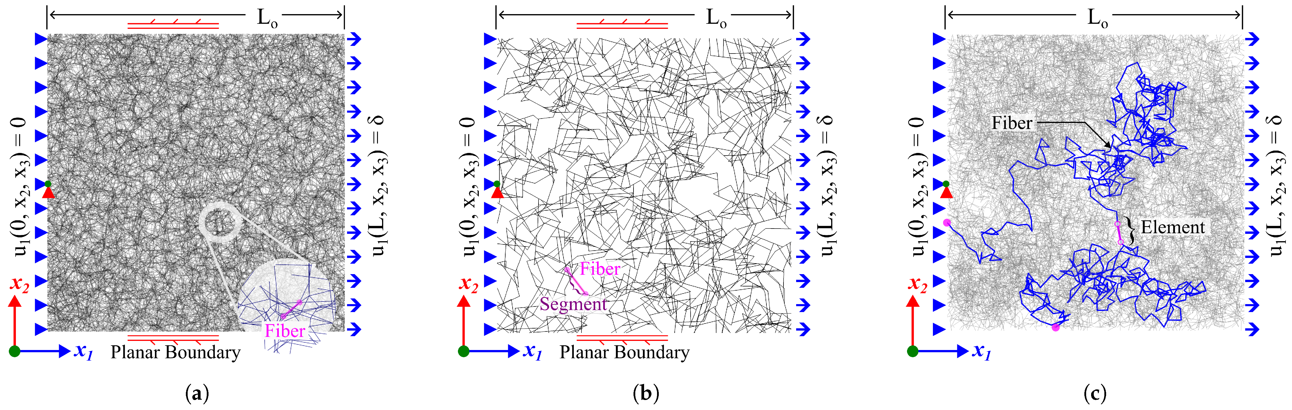
Network materials of cellular type consist of fibers crosslinked only at their ends. Typical examples of network materials of this kind are open cellular foams [46] and many biological collagen networks with . Therefore, these networks can be modeled using the traditional Voronoi tessellation procedure in 3D. For this purpose, a 3D cubic space of edge length is populated with random seed points following a uniform distribution. The edges of the Voronoi tessellation [47] generated from these seeds are treated as fibers and their merging points are retained as crosslinks. Thus, the fibers are initially straight with . The model is then trimmed to the desired cubic shape of edge length . This final step reduces the boundary effects associated with the tessellation procedure. An example of the final model, along with a magnified fiber, is shown in Figure 1a.
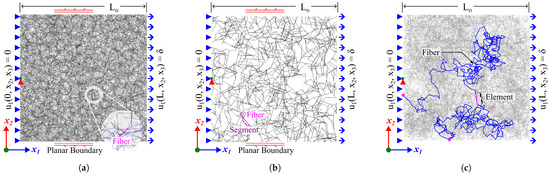
Figure 1.
Example of fiber network models considered in this work: (a) cellular (Voronoi), (b) fibrous (Mikado), and (c) crimped fibrous network (CFN) with single fiber highlighted. The 3D CFN and Voronoi networks are visualized in 2D. The Mikado network in (b) is 2D. All network models are represented in cubic/square domains of edge length with planar boundaries applied to selected cases.
The length of the fibers in this architecture is Poisson distributed, thus the mean length, , fully characterizes the distribution. To improve the computational efficiency in explicit dynamic simulations, we remove fibers with length by merging the associated crosslinks. Typically, fibers shorter than this limit are quite stiff in bending, so this modification does not alter the mechanics of the network. The procedure also increases the connectivity of a small subset of the crosslinks but does not affect significantly. Finally, any dangling fibers created up to this point that are not at the boundary do not contribute to the strain energy and are removed from the model.
Due to the uniform distribution of the seed points, the network does not have any preferential alignment of fibers in the initial configuration. The number of these seed points and the model size are thus the primary parameters for the model generation. The characteristic non-dimensional parameter of the network is , with line density, , measured in the reference configuration. For , the deformation of the network is controlled by the bending deformation modes of fibers and shows increasing degrees of non-affinity as decreases [24].
2.2. Fibrous (Mikado) Network Generation
Fibrous networks concern network material where fibers of pre-specified lengths are embedded in space with crosslinks at their initial contact points. We model this in 2D using a Mikado-type architecture that closely resembles the micro-architecture of paper [1,18,48]. The model is generated by depositing straight fibers of fixed length oriented at random angles in a target square domain of edge length, . The location and orientation of the deposited fibers are controlled by two parameters: the centroid of the fiber and the angle it makes with a reference axis. The values for both of these parameters are drawn from a uniform random distribution. The intersections of the deposited fibers are treated as crosslinks. Thus, a fiber can form crosslinks with multiple neighbors. The fiber segments protruding out of the model domain are then trimmed to obtain the desired model. Finally, we remove dangling segments of the fiber that are not part of boundary faces to reduce computational cost and dynamic effects. These segments are the fundamental components of this network in subsequent numerical procedures. The segment lengths are Poisson distributed. An example of such a model is provided in Figure 1b with a single fiber highlighted.
This network has average connectivity and no preferential alignment in the undeformed configuration. We characterize the non-affinity of the model using a non-dimensional parameter, , with the transition from non-affine to affine deformation mode occurring at . The overall generation process is therefore controlled by two parameters: length and number density of fibers. Finally, here we consider two types of constitutive behavior of the fibers for this architecture: linear elastic and time-dependent linear viscoelastic. This provides us with the opportunity to investigate the effect of mesh refinement on the viscoelastic response of the overall network.
2.3. Crimped Fiber Network (CFN) Generation
Most naturally occurring fibers are wavy. Although the mechanical behaviors of the network with crimped fibers are qualitatively comparable to those with straight fibers [26], the presence of crimps affects the microscopic details of the deformation. Hence, in special cases, the waviness of the individual fibers needs to be modeled explicitly. The crimped fiber network model we present here consists of many such initially crimped fibers generated using random walk following the procedure described in [19]. A starting point is selected on one of the model boundaries and steps of the same length are taken inward of the domain. The direction of each step is selected at random within a cone of axis defined by the previous step’s direction. The apex angle of the cone controls the degree of directionality of the walk and its persistence length, . This process continues until the random walk reaches a boundary. The number of fibers generated, step length, and the minimum fiber length are part of the model generation parameters.
After the fiber generation process, the model is trimmed to the desired size and then crosslinks are added based on a proximity criterion while avoiding crosslinking a fiber with itself. One such fiber is shown highlighted in Figure 1c. This crosslinking approach ensures adequate crosslinking between the fibers and also dictates the maximum length of the crosslinking connector elements. The crosslinks are modeled as stiff linear springs. Finally, fibers with no crosslinks and fibers’ dangling ends are removed to avoid unnecessary segments that do not store strain energy. The nodal connectivity z is nominally 4, although a small fraction of crosslinks with exists after dangling ends are removed.
2.4. Simulation Procedure and Boundary Conditions
For networks with linear elastic fibers that we study, the relevant material parameters are Young’s modulus, , shear modulus, , and fiber material density, . We also investigate the effect of time-dependent viscoelastic relaxation in selected cases. In all cases, the fiber segments are modeled as initially straight beams and are discretized using Timoshenko beam elements of first or second order [30]. Thus, all nodes have 6 degrees of freedom: 3 translational and 3 rotational. Due to the Poisson-distributed fiber segment length, we expect beams with a large range of aspect ratios, so this formulation is preferred over the Euler–Bernoulli one. One may, however, also consider higher-order beam models such as in Refs. [49,50]. The beam cross-section is assumed to be constant during deformation. We also do not consider inter-fiber contacts or frictions, as their effects are negligible in tension due to the large free volume of network materials [34].
All the results presented here are based on finite element simulations solved using the ABAQUS finite element software package [51]. We seek the static solution for the network deformation as a function of applied stretch. We employ a linear perturbation procedure to obtain small strain responses. An implicit method does not apply to finite strain analysis of the network model since network deformation beyond a few percent strain entails microstructural reorganizations (large local deformations and rotations) that cannot be resolved using such methods. Consequently, we use an explicit forward marching technique (ABAQUS/Explicit) to obtain the quasi-static solution. The numerical formulation accounts for the effects of geometric non-linearities of the deformation. To assert the validity of the quasi-static assumption, we monitor the kinetic and strain energy of the model so that the kinetic-to-strain energy ratio stays below 5% following recommendations from [51]. This is typically not maintained at the early stage of simulation (up to approx. 2% nominal strain) due to start-up effects. To improve the energy balance and subsequent stability, we introduce an otherwise negligible viscous damping to the system. The energy associated with viscous damping is also monitored to ensure it is negligible compared to the overall strain energy.
The dynamic explicit simulation procedure utilizes a central difference-based forward time marching algorithm. The applicable stable time increment is defined in terms of the highest frequency in the system, which can be approximated as the ratio of the characteristic length of the elements and wave speed in the fiber material [51]. The characteristic length equals the length of the element for first-order and half-length for second-order beam element formulation. The longitudinal wave speed, on the other hand, is computed from fiber material property as . This, in general, leads to a quite small step time in the numerical integration schemes due to Poisson-distributed fiber lengths and/or constraints on material parameters. Specifically, the length of shorter fibers determines the time step at which the integration scheme can proceed. To improve computational efficiency, we artificially increase the mass density of the short elements in addition to the element removal described earlier, while ensuring that the inertia forces are much smaller than the forces transmitted between elements. This is acceptable within the quasi-static solution sought here. Finally, the simulation outputs also depend on the nature and magnitude of the strain rate (i.e., load amplitude curve) but it is not critical as long as the quasi-static condition is maintained. We choose these simulation parameters at a balance between computational efficiency and accuracy.
For uniaxial tension tests, we load the network model in tension under displacement control and with a constant engineering strain rate. To this end, displacement boundary conditions are prescribed to all nodes belonging to one of the boundaries while the nodes of the opposite boundary are constrained in translation along that direction. To prohibit rigid body motions, a single node on this ‘fixed’ boundary is constrained in all available translational and rotational degrees of freedom. For boundaries perpendicular to the loading direction, we consider two possibilities. (i) Free: the boundary nodes are traction-free (strong-free), or (ii) planar: the nodes are kinematically tied such that the boundary plane remains planar (weak-free). In the second scenario, the relevant boundaries are still free to move in their direction to their normal. As a result, the reaction force at the respective boundaries is zero in the average sense. Planar boundaries provide two advantages: they stabilize the deformation by removing spurious network kinematics that may appear close to the boundaries, particularly in small models, and allow facile estimation of the deformation gradient (and Poisson contraction) at all strains. The deformation gradient is useful, for example, when computing the incremental non-affinity of the network. The boundary conditions are shown schematically in Figure 1 for the three network architectures discussed.
To investigate the linear viscoelastic behavior in the relaxation mode, a fibrous Mikado network (, non-affine) is subjected to uniaxial tension up to a stretch value of . Following this, the overall strain is maintained at a constant level while observing the stress, in the loading direction as a function of time, t. Forces acting in directions perpendicular to the loading direction are maintained at zero. The network behavior during loading is restricted to being elastic with no relaxation, although non-affine, to facilitate the interpretation of the subsequent relaxation response. Subsequently, the constitutive model transitions to a viscoelastic representation to capture the ensuing relaxation phenomenon. The viscoelastic material is described using a Maxwell model [52] incorporating a relaxation time constant .
2.5. Mesh Refinement Strategies
In this section, we elaborate on the p and h-refinement of the finite element meshes. Here, p-refinement refers to increasing the order of interpolating polynomials in finite elements. We focus on two flavors of Timoshenko beam element formulation available in ABAQUS: 2-noded linear and 3-noded quadratic elements denoting first and second-order polynomials used to approximate the displacement field, respectively. The details of their analytical formulation can be found elsewhere, e.g., [30,51,53].
The h-refinement concerns the discretization of the geometry. The h-refinement for Mikado and Voronoi network is discussed in terms of fiber segment length, i.e., the span of the fiber between two adjacent crosslinks, denoted by l. This is equal to the fiber length for the Voronoi network. To begin, all fiber segments are represented by a single element of specified order. We refine the mesh by uniformly splitting all segments into a fixed number of elements, s. The new elements are created by introducing nodes in-between the terminal crosslinks through linear interpolation such that all elements belonging to a segment are of equal length, . Thus, the element length distribution is the same as the segment length distribution, scaled by s.
For the Voronoi network, we further consider mesh refinement based on the ratio of fiber segment length to their mean value, i.e., , to selectively discretize the longer slender fibers only. We define this refinement strategy by two parameters: as the minimum r beyond which a segment may be refined, and as the maximum number of elements per segment after said refinement. For a fiber, if the condition is met, the number of elements after refinement is determined by rounding r to the nearest integer. Thus, a long fiber may be discretized into at most elements while those shorter than will be represented by a single element. Note that the rounding operation and Poisson-like fiber length distribution tend to limit the impact of and on the discretization. Similar to the previous strategy, discretization is accomplished by introducing additional nodes such that all elements belonging to a fiber have equal length, here computed as if is satisfied, otherwise . Thus, the element length distribution is similar to the fiber length distribution at the low end of but truncated at the other end.
In the discussion to follow, we denote the uniform mesh refinements with the notation (element order, number of elements/segment, condition on the boundary perpendicular to loading direction). We use the letter ‘L’ for linear and ‘Q’ for quadratic elements. The number of elements per segment is a positive integer. The planar and free boundaries are indicated by ‘p’ and ‘f’, respectively. Thus, mesh[] indicates each fiber segment is discretized using 3 quadratic beam elements and the boundaries perpendicular to the loading direction remain planar. For length-based adaptive discretization, we replace number of elements/segment with (, ). In this notation, mesh[], for example, indicates fibers are modeled using linear beam elements with segments longer than discretized into at most 3 elements (otherwise 1 element/fiber segment) and the boundaries are traction-free. Among all the refinements considered, the mesh[] is the most computationally intensive with 11 nodes/segment, hence it is taken here as the reference solution for the subsequent discussions unless otherwise specified.
For CFN, the fibers start and end from/to the model boundaries. Therefore, each fiber has multiple crosslinks with other fibers, and using multiple elements per fiber becomes an obvious necessity. Due to the generation procedure and computational considerations, the smoothness of the crimps is generally limited. This directly relates to the wavelength of the waviness of the fibers. Here, we design a refinement protocol to investigate this aspect of the model. To this end, the fibers are generated with fine step sizes, , in the constrained random-walk process. We then merge adjacent elements to create progressively coarser meshes. Here, we present four levels of coarsening in which 2, 4, 8, and 16 steps of the random walk are bunched together in separate models and represented with a single element of length equal to the end-to-end vector of the respective segments. All elements are represented using quadratic beams in the simulation.
3. Results and Discussions
3.1. Small Strain Analysis
The small strain stiffness, , measures the linear response of the network material under an uniaxial perturbation. This stiffness normalized by the affine prediction, e.g., , is generally presented relative to a structural parameter such as w, the so-called master curve [25]. For non-affine networks of small w, is proportional to the bending rigidity of the fibers, , and to axial rigidity, for affine networks of large w. Here, and denote the cross-sectional area and axial moment of inertia of the fibers respectively. Thus, the master curve has two distinct regimes of small and large w separated by a threshold, , denoting the affine to non-affine transition. To start the discussion, we first look at the effect of mesh refinement on this master curve.
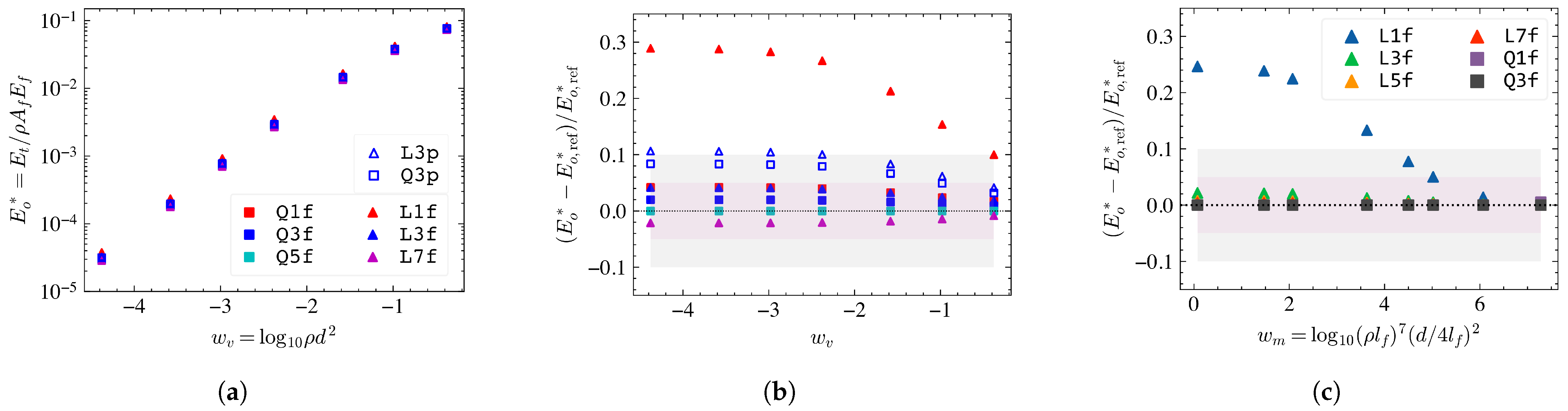
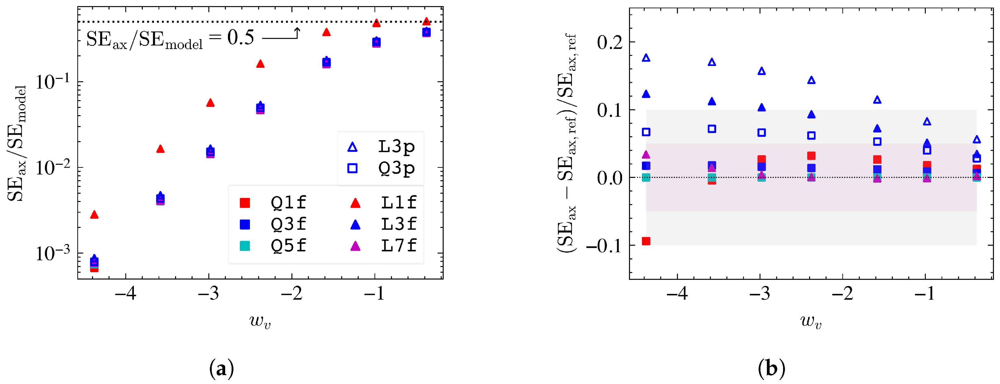
The master curve for Voronoi networks is shown in Figure 2a with respect to the relevant non-affinity measure, , for a variety of mesh discretizations. We find that all levels of mesh refinement recover the expected behavior. However, the relative differences between the discretizations are hard to distinguish due to the logarithmic scale of the vertical axis. To verify the mesh convergence, we compute the relative errors of with 5 quadratic element/fiber segments, i.e., mesh[] (11 nodes/segment) taken as reference, and show the results in Figure 2b. We choose arbitrary thresholds of and to be the desired and acceptable bounds. These thresholds are marked in the figure with shaded regions. The results indicate that using meshes with one linear element per segment, mesh[] leads to an overestimation of the model stiffness by as much as 30% in the non-affine regime. Interestingly, the discrepancy is limited to this mesh only, and all other free boundary cases fall within a relative error margin. Finer mesh leads to better agreement with the reference result for both linear and quadratic elements. We also note that the effect of the planar boundary is to increase the stiffness of the model in the non-affine range of . The equivalent data for Mikado networks is shown in Figure 2c with respect to . Here too, using a mesh with a single linear element per fiber segment leads to larger errors. In this case, however, h-refinement beyond three nodes per fiber segment, e.g., mesh[], does not bring any noticeable improvement.
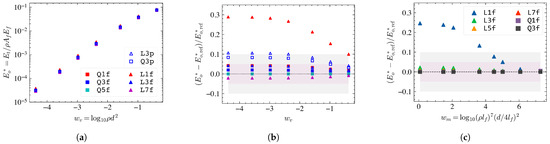
Figure 2.
(a) Small strain stiffness normalized by the affine prediction of the stiffness, , presented as a master curve for 3D Voronoi network. (b) The relative error in normalized network stiffness, for Voronoi with results from fiber segments modeled with five quadratic elements, i.e., mesh[] taken as the reference (denoted as ). The markers in panel (b) have the same meaning as panel (a). The pink and gray shaded regions correspond to and relative errors, respectively. (c) The relative error in normalized stiffness for fibrous Mikado network with respect to mesh[].
The cause of the aforementioned deviations can be traced to the effective stiffness of the elements. In finite element analysis, coarser meshes tend to produce stiffer model responses due to a smaller number of degrees of freedom. As a result, the energy partition in the fibers is skewed away from the softer bending mode in progressively coarser meshes. Figure 3a shows the fraction of axial energy in the Voronoi networks for several mesh refinements. The results indicate that mesh[] stores a larger fraction of the strain energy in the axial mode than all other cases considered. An important implication of this result is the estimation of the affine to non-affine transition point, . A model may be considered affine if the energy is stored predominantly in the axial mode at small strains, i.e., with corresponding to . The mesh[] predicts while mesh[] and beyond indicates for the Voronoi network.

Figure 3.
(a) The fraction of the axial component of the strain energy in the small strain regime of Voronoi network as a function of and (b) the respective relative errors for various discretization considered. The fraction of the axial strain energy computed with the mesh[] is taken as reference in panel (b). Note, the relative error associated with mesh[] is larger than 25% for all considered here. The legends from (a) apply to both panels.
The relative error computed with mesh[] as a reference in Figure 3b better shows the effects of mesh refinement on the fraction of axial strain energy stored in the network. Not surprisingly, mesh[] falls outside the range of relative error shown in the figure, underscoring the overwhelmingly axial deformation mode prevalent in this case. Further, mesh[] tends to overestimate shear and torsional deformation mode contributions. We find similar distortion of energy balance for mesh[] and mesh[] as well, though within bound. These deviations in the non-affine portion of the master curve are generally at the cost of the softer bending energy of the model, leading to a larger model stiffness. The same argument also explains the stiffer response associated with planar boundary conditions.
Since non-affinity is an integral feature of fiber network deformation, we advise avoiding meshes with a single linear element per fiber segment in the numerical simulation of discrete fiber networks, especially for non-affine models. Based on the data presented here, we recommend finite element meshes with at least three nodes per segment in linear analyses.
3.2. Finite Strain Analysis
In the absence of dissipation, fiber network materials often exhibit hyper-elastic behavior with respect to applied stretch, . In such athermal systems, the nominal stress, S, and tangent stiffness are derived from the strain energy. Thus, we expect the relative errors and numerical noise to be elevated for tangent stiffness compared to nominal stress and energy. Further, the non-linear behavior of network materials is w dependent [1,26,34]. For example, Voronoi networks with exhibit three distinct stiffening regimes under finite strain. In Regime I, the material response is approximately linear elastic, followed by exponential stiffening in Regime II () and Regime III (). We, however, note that Regime III is not observed when the Cauchy (true) stress is used to evaluate the stiffness-stress plot; in this case, is proportional to the Cauchy stress beyond Regime I [54]. For affine networks (large w), the exponential Regime II is nonexistent. We found mesh refinement to be most critical in Regime II of non-affine networks. In this section, we present the results for the non-affine Voronoi network (), followed by fibrous Mikado architecture (, non-affine). We briefly discuss affine models in Section 3.8.
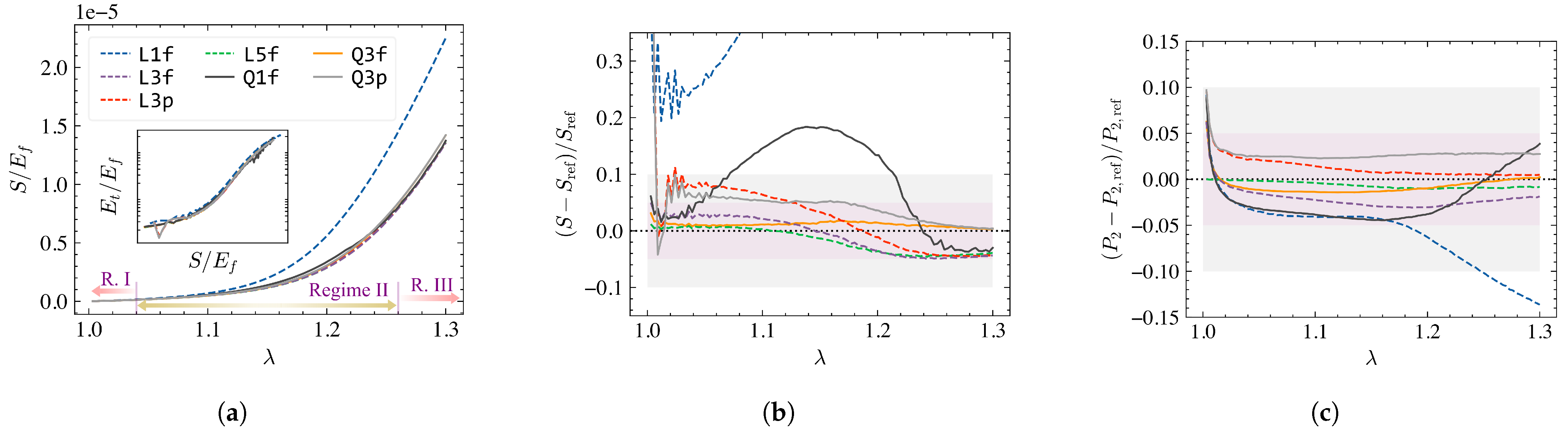
The stress productions in Voronoi networks for various levels of uniform mesh refinement are shown in Figure 4a. Similar to the small strain analyses, we observe a significant deviation when a single element is used to model a fiber segment, i.e., mesh[]. To further investigate small to moderately large strain response, we report in Figure 4b the relative errors computed with mesh[] as reference. Clearly, mesh[] over-estimates the nominal stress by at least 25% compared to the reference. The refined linear meshes also tend to over-estimate the nominal stress at smaller strains (Regime I and II), and under-estimate at larger strains (Regime III), but remain within an acceptable margin. Interestingly, the quadratic mesh[] shows a large deviation from the reference result, especially in Regime II. Such deviation is due to a combination of (i) the availability of the first bending mode and (ii) the large reorientation of fibers in the loading direction. This result highlights the importance of the flexibility of fibers in the numerical convergence of network analyses.
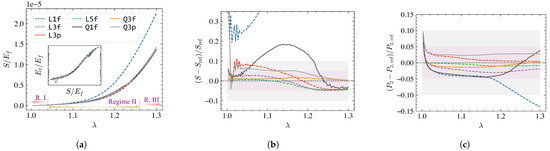
Figure 4.
(a) The nominal stress-stretch response of a 3D non-affine Voronoi network under uniaxial tension test with various levels of mesh refinements. The inset shows the tangent stiffness vs. stress for all curves in the main figure. The stiffening regimes shown in the main figure are identified based on changes in the tangent of stiffness vs. stress data. The relative errors in (b) nominal stress and (c) average element orientation are computed with respect to the result of a model with five quadratic elements per fiber, mesh[]. The legends from (a) apply to all panels.
The relative errors in the predicted tangent stiffness show trends comparable to those observed for stress from Figure 4b for various discretizations considered. The magnitude of the relative error, however, increases by approximately 10–20% depending on the level of refinements. Regardless, all meshes produced comparable functional forms of the stiffening behavior. This is shown in the inset to Figure 4a where the tangent stiffness vs. stress is plotted for the discretizations considered here.
One of the primary motivations behind discrete fiber network simulation is access to the micromechanical details of the deformation process. Here, we comment on the effect of mesh refinement on the mean reorientation of the fibers. This is quantified through for a 3D Voronoi network [1,55]. In the expression, denotes the angle between the tangent to a fiber direction and the global loading direction. We compute this quantity at the length scale of elements to reduce computational complexity. The tangent vectors are thus approximated using the terminal nodes of the individual elements, with the average performed over all available elements in the model. The relative errors computed with mesh[] as reference are presented in Figure 4c. We find that all mesh refinements provide results within an acceptable error margin. However, predictions obtained with meshes with a single element per fiber segment (e.g., mesh[] and mesh[]) diverge near the middle of Regime II and on a trend outward of the bound. The stiffer response of the fiber segment and error associated with approximation of tangent in mesh[] are the contributing factors for these deviations. Still, the kinematic variables are less affected by discretization levels in an average sense than the energetic quantities discussed earlier.
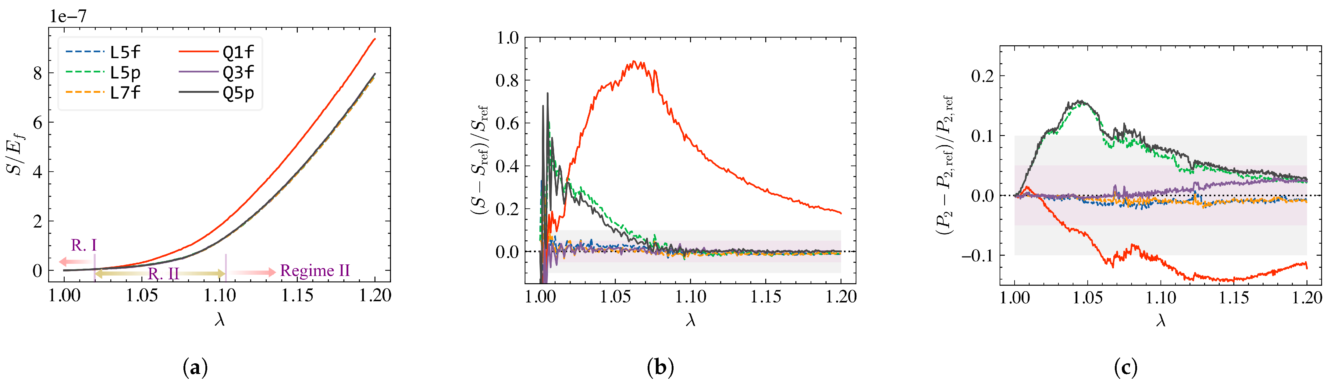
A similar set of results from the large strain analysis of the fibrous Mikado network indicates a more strict mesh refinement requirement. The constitutive responses for a Mikado network with are shown in Figure 5a. The stress response for mesh[] diverges noticeably from all other cases. The relative errors in stress computed in Figure 5b with respect to mesh[] indicates a maximum of 90% deviation at early stages of Regime II for this mesh, rendering the results unacceptable. A similarly large deviation for this mesh is observed in as well, here computed as at the element scale (Figure 5c). Finally, the planar boundary conditions led to a significant level of error until mid of Regime II, regardless of the discretization.
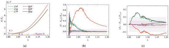
Figure 5.
(a) The nominal stress–stretch response of a 2D non-affine Mikado network under uniaxial tension test for various discretizations with the stiffening regimes shown. The relative errors in (b) nominal stress and (c) average element orientation are computed with respect to a model with five quadratic elements per fiber, i.e., mesh[]. The legends from (a) apply to all panels.
Based on these results, we recommend using finite element meshes with at least six nodes per segment for non-affine fibrous network simulations if the uniform mesh refinement strategy is employed. Planar boundary conditions should be avoided unless essential. We provide a mesh recommendation for the cellular Voronoi network model in Section 3.7.
3.3. Viscoelastic Relaxation
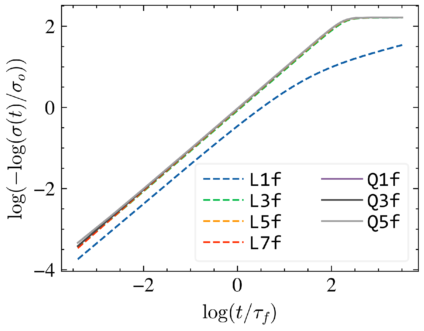
In a prior investigation, a connection between the structural parameters of the network material and its viscoelastic relaxation characteristics was established [42]. The analysis was conducted for both 2D Mikado Networks and 3D Voronoi Networks. Nonetheless, the concept of mesh refinement was never explored in that study. As in [42] and to facilitate the interpretation of the network scale response, here we consider Mikado networks of fibers made from a linear viscoelastic material with a single time constant, . The model is stretched uniaxially up to 3% strain after which the strain is kept constant, and stress relaxation is monitored. The variation in the stress in time, , is plotted in Figure 6 after normalization with the stress at the onset of relaxation (at the end of the loading period of 3% strain), , and rearranging as vs. . In this representation, an exponential relaxation with a single time constant would appear as a straight line of Slope 1 and the intercept equals the log of the network scale relaxation time. Figure 6 shows the stress during the relaxation regime for various mesh refinement levels. It is seen that using a single linear element per fiber segment leads to erroneous results, while any other higher level of mesh refinement provides converged curves. For similar analyses with larger strain at the end of the loading phase, we recommend following the best practices for the underlying Mikado network architectures discussed in the previous section.
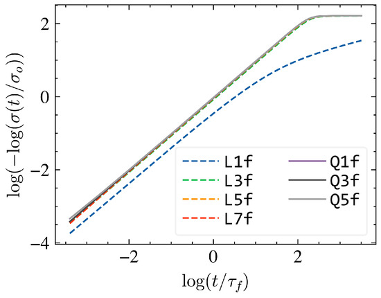
Figure 6.
The normalized linear viscoelastic relaxation of the 2D Mikado network for the various levels of discretizations.
3.4. Crimped Fiber Network (CFN)
The models with crimped fibers discussed in Section 2.3 belong to the class of fibrous networks. Fibers are defined by directed random walks in 3D which begin from one model surface and end on another surface, with the restriction that the endpoint of a fiber should not be on the model face directly opposite to the face from which the walk began. Let be the length of the random walk step. The directed walk is characterized by the persistence length, . The persistence length defines the rate of decay of the tangent vector auto-correlation function measured along a fiber [1]. Fibers are crosslinked based on a proximity criterion, and the crosslink density is adjusted by controlling the threshold distance below which two segments are connected. The contour length between crosslinks measured along a fiber, , is another characteristic length of the structure. These three characteristic lengths largely control the stiffness and overall mechanics of the network. Specifically, must be about one order of magnitude smaller than for the walk to resolve the desired tortuosity. Further, if , segments are approximately straight on length scales defined by the crosslink to crosslink distance (mesh size) and the situation becomes comparable to the Voronoi networks discussed earlier.
If , the network is very soft if entanglements (topological constraints associated with the condition that fibers should not cross) are not enforced. The situation of more interest is that in which is larger, but comparable with . This is the case considered here and, for this scenario, we study the effect of mesh refinement. We consider systems with equal to 10 steps of the random walk and crosslink the walks (fibers) such that is equal to 30 steps. Hence, . In the reference configuration, each step of the walk is represented with a single quadratic finite element and, in this case, and , with being the element length. The discretization is gradually coarsened such that , in separate models. This coarsening is performed by representing 2, 4, 8, and 16 steps of the random walk with one straight element, respectively, while maintaining constant. In this process, the fine-scale features of the walk are gradually eliminated.
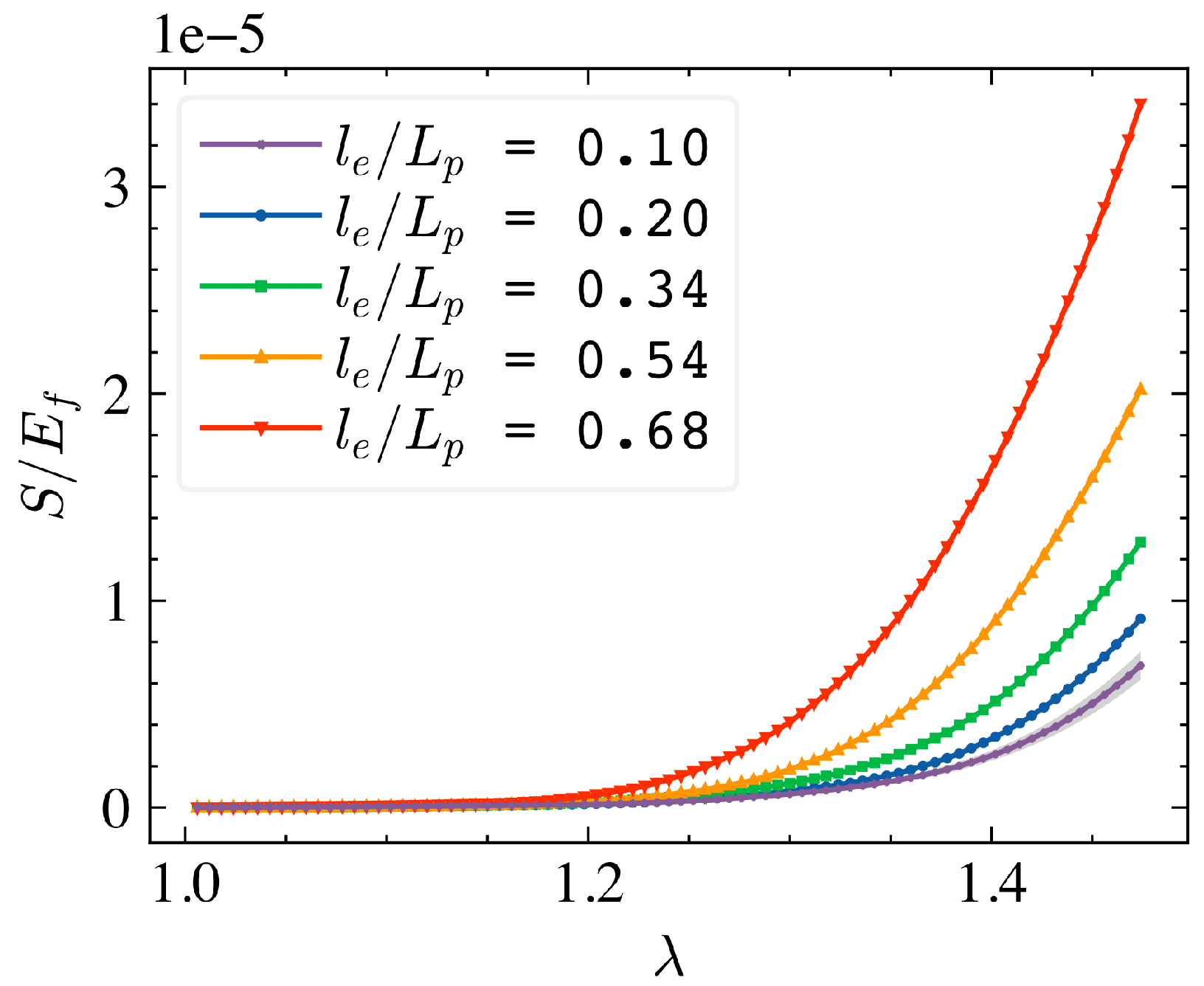
Figure 7 shows the nominal stress vs. stretch for several models with various . The response becomes stiffer as the degree of coarsening increases. However, the functional form of stiffening does not change and remains exponential. The first level of coarsening, , provides a curve that is within 10% from the reference curve ( in Figure 7) up to a strain of 20%. The 10% error range is shown as a shaded band around the reference curve. is within 25% of the reference up to 40% strain. All coarser meshes provide gradually less accurate solutions for specified . For further discretization of walk steps, the microstructure becomes comparable to the Voronoi network model, and conclusions from Section 3.2 apply.
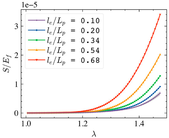
Figure 7.
Finite strain response of 3D crimped fiber network for four levels of mesh refinement, defined by the ratio of the element length, , to the persistence length, . In the most refined case taken as the reference here, the response is softest (lowest curve) and . The shaded region corresponds to 10% deviation from this reference result. Curves corresponding to increasing degrees of coarsening and increasing values are gradually stiffer.
Based on these observations, we recommend that, as long as the fiber is generated as a directed random walk, one quadratic element per walk step should be used. If the fiber is generated as a smooth contour in space (e.g., analytically), as a starting point of the evaluation of the effect of discretization, we recommend 10 elements per .
3.5. Adaptive Meshing
So far, we have shown that discrete fiber network simulation results tend to converge as the finite element mesh becomes more refined or the order of the element increases. This, however, comes with an increasing computational burden due to the large number of degrees of freedom introduced. Further, uniform mesh refinement discussed in the previous sections creates elements with progressively shorter lengths, leading to smaller time steps in explicit integration schemes. At the same time, we also identified the flexibility of fibers as an important factor for numerical accuracy in the discussion of Figure 4b. As an alternative, here we explore the length-based adaptive meshing techniques mentioned in Section 2.5. The following discussion pertains to a non-affine Voronoi network, but we expect the conclusions and recommendations to be equally applicable to other network architectures.
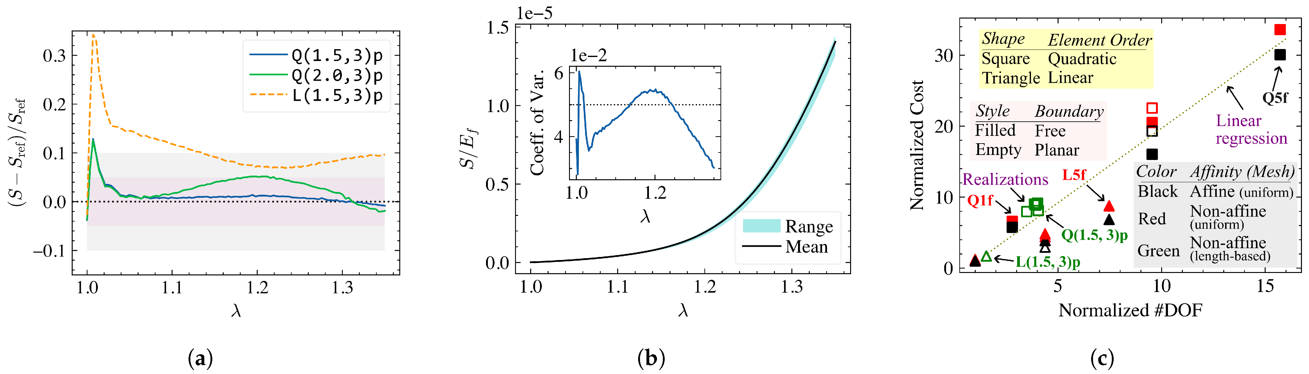
The adaptive meshing is well suited for network materials due to the Poisson-distributed fiber segment lengths. Since the algorithm selectively discretizes the longer (slender) fibers, the quality of the solution improves with little to no change in the time step used in the integration scheme The relative errors in stress response of a non-affine Voronoi network are shown in Figure 8a for a few selected adaptive discretization strategies with the results of mesh[] taken as reference. Here, fibers with length (mesh[], mesh[]) or (mesh[]) are discretized into at most three elements per fiber following the procedure described in Section 2.5. The output of mesh[] is comparable to the more computationally intensive reference discretization. The more interesting case, however, is the mesh[] given the large relative error we observed for mesh[] in Figure 4. This clearly shows that it is the slender fibers that control the accuracy of the solution in non-affine networks.

Figure 8.
(a) The relative error in stress for several length-based adaptive mesh refinements computed with respect to mesh[]. The notation mesh[] indicates that fiber segments longer than are discretized into at most 3 elements, and the boundaries remain planar during deformation. A complete description of the notations is provided in Section 2.5. (b) The average stress response and corresponding min/max range from 6 realizations of network models with mesh[] discretization. The coefficient of variation (CV) is shown as inset with 5% CV marked with a dotted line. All results in (a,b) are for non-affine Voronoi networks subjected to large deformations (up to stretch, ). (c) The approximate computational cost incurred for dynamic explicit simulations. The available degrees of freedom (horizontal axis) and the cost (vertical axis) are normalized by the corresponding values pertaining to mesh[].
For the discretizations considered in Figure 8a, the largest errors are observed in the small strain regime. This is a consequence of the initially straight fiber assumption and may be safely overlooked, especially for mesh[]. To the authors’ best knowledge, all available meshing packages include some form of length-aware adaptive h-refinement capability, so this technique is recommended for general discrete fiber network simulations. Alternatively, the basic adaptive meshing techniques described in Section 2.5 may be easily implemented using freely available programming languages such as Python [56].
3.6. Ensemble Averaging and Size Effect
Studies on fiber networks of finite size generally demand averaging over many realizations (embedding and connectivity generated from different random seed points) due to the underlying stochasticity. This becomes especially important if the ratio of the model size to a characteristic length scale of the network is below a model-dependent threshold. The characteristic length scale of the network may be the smallest length of interest (mean fiber length, for example) or the characteristic length of embedded defects (e.g., pre-existing cracks). If fiber damage is considered, the size effect controls the failure mechanism to a great extent [57,58]. For pure elastic analyses, the effect of boundary nodes may have an undue influence on the deformation of interior fibers, hence rendering the material response overly sensitive to the model parameters. A plethora of published works discusses these issues under the umbrella term boundary and size effects. We follow the recommendations in [25,59] for all network architectures considered. For example, the characteristic length scale in our Voronoi network model is the mean fiber length, and we maintain following the results of [59].
To further investigate the necessity of multiple realizations, we consider six realizations of a non-affine Voronoi network with mesh[] and . The line density, (thus ) changes with the realizations but remains within a very tight tolerance (coefficient of variation: 0.01). Consequently, the stress response remains very close, as shown in Figure 8b. The coefficient of variation in the stress response is shown as an inset of Figure 8b which has a maximum of approximately 5% beyond the start-up effect and appears near the transition between Regimes II and III ( this model). When we reduce the model size to , the coefficient of variation increases to a maximum of 14% at the same stretch, underscoring the necessity of large models in numerical simulations.
Therefore, to investigate the asymptotic response of fiber network materials, we recommend larger models so that the size effect is as small as feasible, thus eliminating the need for multiple replicas and associated computational costs.
3.7. Computational Cost
A recurring theme in this work is the balance between computational cost and solution accuracy. To provide further guidance, we estimate the total computational cost the product of the number of CPU cores used in the simulation and the total compute time. In an explicit integration scheme, a linear relation between degrees of freedom and computational cost is expected. However, algorithm/hardware architecture dependency and parallel overheads will lead to significant variations across computing environments. With the specifics of our approach (see Section 2.4) in mind, we plot the computational cost incurred with respect to available degrees of freedom in the Voronoi network models in Figure 8c. Here, the quantities are normalized by the corresponding values from a model discretized with a single linear element per fiber, i.e., mesh[]. A linear regression line based on the data points pertaining to quadratic elements is shown in the figure for reference. The difference in the trend for linear elements stems from the element characteristic length approximation method used in our analysis package.
Due to the aforementioned particularities and assumptions, this result should be considered only as an initial guidance. Still, we can draw several important conclusions based on this data. First, we find the planar boundary conditions add to the computational cost due to additional constraint equations introduced. We expect this to increase with the number of relevant boundary nodes and model size. Second, the affine models (discussed in the next section) are less computationally intensive, here due to the method of stable time increment selection. Third and most importantly, the length-based adaptive meshing technique produces reasonably accurate results at a fraction of the computational cost of the uniform meshing procedure, e.g., compare mesh[] data shown in Figure 8c to Figure 8a. We thus recommend mesh[] or mesh[] for finite strain analysis of general cellular (Voronoi) networks.
3.8. Other Modeling Aspects
Many properties of fiber networks are related to non-affine deformation. A fiber network may become more affine due to increased fiber volume fraction (implemented by increasing fiber diameter, d, or line density, ) or the persistence of fibers across multiple crosslinks (in fibrous networks, for example). While the affine models are associated with fibers that store energy mostly in their axial deformation mode, non-affine models deal with large deformations controlled by bending. Not surprisingly, the convergence criteria are far less demanding for affine models. The relative error in stress responses for near-affine Voronoi () and Mikado () networks are shown in Figure 9a,b, respectively. Compared to Figure 4b and Figure 5b, we find the affine model outputs to be acceptable with minimum refinement: mesh[] for Voronoi and mesh[] for Mikado. The stability of the numerical models improved with increasing affinity as well, especially for the Mikado architecture. We also note that the network line density, , has a negligible effect on the elastic response as long as w is held constant, and so we expect the conclusions from mesh refinement analyses to be independent of .
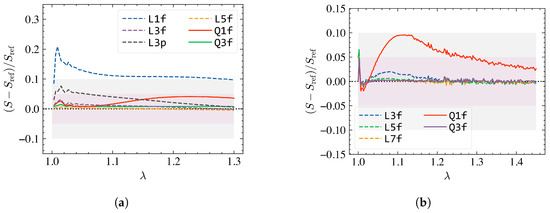
Figure 9.
Relative error in the stress response for near-affine (a) Voronoi () and (b) Mikado network () models. The relative errors are computed in reference to results obtained using mesh[].
All finite strain results presented here maintained a kinetic-to-strain energy ratio of less than 0.05 up to the maximum strain explored. The ratio was maximum for mesh[], approximately 0.02 near the Regime II–III transition. However, the quasi-static assumption was invalidated briefly for this mesh due to large viscous dissipation, as high as 20% of strain energy after said transition. This is related to the availability of the first bending mode in the single element used to model the fiber. At large deformation, fibers realign in the loading direction through significant bending and rotation of crosslinks. Especially for slender elements (equivalent to fibers in mesh[]), this may cause buckling-type instabilities, leading to the observed peak in viscous energy. Reducing or modifying the strain rate (e.g., using a graded/quadratic ramp in place of a linear load amplitude curve) helps but does not fully eliminate this issue. For higher levels of mesh refinements, however, the probability of such element-level instabilities decreases, thus fully resolving this problem. Therefore, mesh refinement improves both the accuracy and stability of numerical simulations involving discrete fiber networks. Finally, as with convergence, affine models tend to be more stable except when . In such cases, inter-fiber contact and fine-tuning model/simulation parameters are generally necessary from our experience.
4. Recommendations and Conclusions
The finite element method is a versatile tool for numerical experiments of discrete fiber network models with complex microstructural features. Through a systematic investigation, this work explored the effects of finite element meshes on the accuracy and acceptability of the results, both for purely elastic and viscoelastic responses. Our recommendations for obtaining accurate and efficient solutions are summarized below:
- Single linear element per fiber segment is a poor choice for both small and finite strain analysis of network materials. This mesh tends to overestimate both the nominal stress and tangent stiffness.
- A single quadratic element per segment is acceptable for small strain approximation, but a higher level of refinements is recommended for finite strain analyses.
- Shorter fiber segments control the applicable time steps in the integration schemes while longer fibers control the overall solution accuracy. Thus, a significant computational effort can be spared by using a segment length-based adaptive meshing strategy.
- Finer meshes tend to improve both the accuracy and stability of numerical models.
The finite element discretization recommendations are provided in Table 1. We expect this report will help future researchers to estimate the necessary model parameters in numerical experiments involving fiber network materials.

Table 1.
Mesh recommendations for finite strain analysis of several discrete numerical models. For perturbation analysis, mesh[] is adequate for most purposes. Planar boundary conditions are recommended if effective deformation gradients and related quantities are of primary interest. Guidelines for crimped fiber networks are provided in Section 3.4.
Author Contributions
Conceptualization, N.P. and C.R.P.; methodology, N.P., S.N.A., M.K.D., and C.R.P.; formal analysis, N.P., S.N.A., M.K.D., and C.R.P.; investigation, N.P., S.N.A., M.K.D., and C.R.P.; resources, C.R.P.; data curation, N.P., S.N.A., and M.K.D.; writing—original draft preparation, N.P.; writing—review and editing, N.P. and C.R.P.; visualization, N.P.; supervision, C.R.P.; project administration, C.R.P.; funding acquisition, C.R.P. All authors have read and agreed to the published version of the manuscript.
Funding
This work was supported by the National Institutes of Health (NIH) through grant No. U01 AT010326-06 and by the National Science Foundation (NSF) through grant CMMI-2022489.
Data Availability Statement
The original contributions presented in the study are included in the article, further inquiries can be directed to the corresponding author.
Conflicts of Interest
The authors declare no conflicts of interest. The funders had no role in the design of the study; in the collection, analyses, or interpretation of data; in the writing of the manuscript; or in the decision to publish the results.
References
- Picu, C.R. Network Materials: Structure and Properties, 1st ed.; Cambridge University Press: Cambridge, UK, 2022. [Google Scholar] [CrossRef]
- Redondo, A.; LeSar, R. Modeling and Simulations of Biomaterials. Annu. Rev. Mater. Res. 2004, 34, 279–314. [Google Scholar] [CrossRef]
- Holzapfel, G.A.; Ogden, R.W. Constitutive Modelling of Arteries. Proc. R. Soc. Math. Phys. Eng. Sci. 2010, 466, 1551–1597. [Google Scholar] [CrossRef]
- Pan, N.; He, J.H.; Yu, J. Fibrous Materials as Soft Matter. Text. Res. J. 2007, 77, 205–213. [Google Scholar] [CrossRef]
- Nguyen, A.T.; Huang, Q.L.; Yang, Z.; Lin, N.; Xu, G.; Liu, X.Y. Crystal Networks in Silk Fibrous Materials: From Hierarchical Structure to Ultra Performance. Small 2015, 11, 1039–1054. [Google Scholar] [CrossRef]
- Holzapfel, G.A.; Gasser, T.C.; Ogden, R.W. A New Constitutive Framework for Arterial Wall Mechanics and a Comparative Study of Material Models. J. Elast. Phys. Sci. Solids 2000, 61, 1–48. [Google Scholar] [CrossRef]
- Melly, S.K.; Liu, L.; Liu, Y.; Leng, J. A Review on Material Models for Isotropic Hyperelasticity. Int. J. Mech. Syst. Dyn. 2021, 1, 71–88. [Google Scholar] [CrossRef]
- Khaniki, H.B.; Ghayesh, M.H.; Chin, R.; Amabili, M. Hyperelastic structures: A review on the mechanics and biomechanics. Int. J. -Non-Linear Mech. 2023, 148, 104275. [Google Scholar] [CrossRef]
- Dal, H.; Açıkgöz, K.; Badienia, Y. On the Performance of Isotropic Hyperelastic Constitutive Models for Rubber-Like Materials: A State of the Art Review. Appl. Mech. Rev. 2021, 73, 020802. [Google Scholar] [CrossRef]
- Picu, C.R. Constitutive Models for Random Fiber Network Materials: A Review of Current Status and Challenges. Mech. Res. Commun. 2021, 114, 103605. [Google Scholar] [CrossRef]
- Chen, S.; Markovich, T.; MacKintosh, F.C. Nonaffine Deformation of Semiflexible Polymer and Fiber Networks. Phys. Rev. Lett. 2023, 130, 088101. [Google Scholar] [CrossRef] [PubMed]
- Heussinger, C.; Frey, E. Floppy Modes and Nonaffine Deformations in Random Fiber Networks. Phys. Rev. Lett. 2006, 97, 105501. [Google Scholar] [CrossRef] [PubMed]
- Wen, Q.; Basu, A.; Janmey, P.A.; Yodh, A.G. Non-Affine Deformations in Polymer Hydrogels. Soft Matter 2012, 8, 8039. [Google Scholar] [CrossRef]
- Di Paola, M.; Failla, G.; Pirrotta, A.; Sofi, A.; Zingales, M. The Mechanically Based Non-Local Elasticity: An Overview of Main Results and Future Challenges. Philos. Trans. R. Soc. Math. Phys. Eng. Sci. 2013, 371, 20120433. [Google Scholar] [CrossRef]
- Shaat, M.; Ghavanloo, E.; Fazelzadeh, S.A. Review on nonlocal continuum mechanics: Physics, material applicability, and mathematics. Mech. Mater. 2020, 150, 103587. [Google Scholar] [CrossRef]
- Eringen, A.C.; Wegner, J. Nonlocal continuum field theories. Appl. Mech. Rev. 2003, 56, B20–B22. [Google Scholar] [CrossRef]
- Licup, A.J.; Münster, S.; Sharma, A.; Sheinman, M.; Jawerth, L.M.; Fabry, B.; Weitz, D.A.; MacKintosh, F.C. Stress controls the mechanics of collagen networks. Proc. Natl. Acad. Sci. USA 2015, 112, 9573–9578. [Google Scholar] [CrossRef] [PubMed]
- Kulachenko, A.; Uesaka, T. Direct Simulations of Fiber Network Deformation and Failure. Mech. Mater. 2012, 51, 1–14. [Google Scholar] [CrossRef]
- Negi, V.; C. Picu, R. Mechanical Behavior of Nonwoven Non-Crosslinked Fibrous Mats with Adhesion and Friction. Soft Matter 2019, 15, 5951–5964. [Google Scholar] [CrossRef]
- Zhang, Y.; DeBenedictis, E.P.; Keten, S. Cohesive and adhesive properties of crosslinked semiflexible biopolymer networks. Soft Matter 2019, 15, 3807–3816. [Google Scholar] [CrossRef]
- Simon, J.W. A review of recent trends and challenges in computational modeling of paper and paperboard at different scales. Arch. Comput. Methods Eng. 2021, 28, 2409–2428. [Google Scholar] [CrossRef]
- Broedersz, C.P.; Mao, X.; Lubensky, T.C.; MacKintosh, F.C. Criticality and Isostaticity in Fiber Networks. Nat. Phys. 2011, 7, 983–988. [Google Scholar] [CrossRef]
- Head, D.A.; Levine, A.J.; MacKintosh, F.C. Distinct Regimes of Elastic Response and Deformation Modes of Cross-Linked Cytoskeletal and Semiflexible Polymer Networks. Phys. Rev. Stat. Physics Plasmas Fluids Relat. Interdiscip. Top. 2003, 68, 1–15. [Google Scholar] [CrossRef]
- Parvez, N.; Picu, C.R. Effect of Connectivity on the Elasticity of Athermal Network Materials. Soft Matter 2023, 19, 106–114. [Google Scholar] [CrossRef] [PubMed]
- Shahsavari, A.; Picu, R.C. Model Selection for Athermal Cross-Linked Fiber Networks. Phys. Rev. Stat. Nonlinear Soft Matter Phys. 2012, 86, 1–5. [Google Scholar] [CrossRef] [PubMed]
- Picu, R.C.; Deogekar, S.; Islam, M.R. Poisson’s Contraction and Fiber Kinematics in Tissue: Insight from Collagen Network Simulations. J. Biomech. Eng. 2018, 140, 1–12. [Google Scholar] [CrossRef] [PubMed]
- Bitzek, E.; Koskinen, P.; Gähler, F.; Moseler, M.; Gumbsch, P. Structural Relaxation Made Simple. Phys. Rev. Lett. 2006, 97, 170201. [Google Scholar] [CrossRef]
- Tauber, J.; van der Gucht, J.; Dussi, S. Stretchy and disordered: Toward understanding fracture in soft network materials via mesoscopic computer simulations. J. Chem. Phys. 2022, 156, 160901. [Google Scholar] [CrossRef]
- Reddy, J.N. An Introduction to the Finite Element Method; McGraw-Hill: New York, NY, USA, 2013; Volume 3. [Google Scholar]
- Belytschko, T.; Liu, W.K.; Moran, B.; Elkhodary, K. Nonlinear Finite Elements for Continua and Structures; John Wiley & Sons: Hoboken, NJ, USA, 2014. [Google Scholar]
- Tojaga, V.; Kulachenko, A.; Östlund, S.; Gasser, T.C. Modeling Multi-Fracturing Fibers in Fiber Networks Using Elastoplastic Timoshenko Beam Finite Elements with Embedded Strong Discontinuities — Formulation and Staggered Algorithm. Comput. Methods Appl. Mech. Eng. 2021, 384, 113964. [Google Scholar] [CrossRef]
- Wang, C.W.; Berhan, L.; Sastry, A.M. Structure, Mechanics and Failure of Stochastic Fibrous Networks: Part I—Microscale Considerations. J. Eng. Mater. Technol. 2000, 122, 450–459. [Google Scholar] [CrossRef]
- Wang, C.W.; Sastry, A.M. Structure, Mechanics and Failure of Stochastic Fibrous Networks: Part II—Network Simulations and Application. J. Eng. Mater. Technol. 2000, 122, 460–468. [Google Scholar] [CrossRef]
- Islam, M.R.; Picu, R.C. Effect of Network Architecture on the Mechanical Behavior of Random Fiber Networks. J. Appl. Mech. Trans. ASME 2018, 85, 081011. [Google Scholar] [CrossRef]
- Heussinger, C.; Frey, E. Stiff Polymers, Foams, and Fiber Networks. Phys. Rev. Lett. 2006, 96, 017802. [Google Scholar] [CrossRef]
- Kakaletsis, S.; Lejeune, E.; Rausch, M. The mechanics of embedded fiber networks. J. Mech. Phys. Solids 2023, 181, 105456. [Google Scholar] [CrossRef]
- Hewavidana, Y.; Balci, M.N.; Gleadall, A.; Pourdeyhimi, B.; Silberschmidt, V.V.; Demirci, E. Assessing Crimp of Fibres in Random Networks with 3D Imaging. Polymers 2023, 15, 1050. [Google Scholar] [CrossRef]
- Scharcanski, J.; Dodson, C.T.J.; Clarke, R.T. Simulating Effects of Fiber Crimp, Flocculation, Density, and Orientation on Structure Statistics of Stochastic Fiber Networks. Simulation 2002, 78, 389–395. [Google Scholar] [CrossRef]
- Dhume, R.Y.; Barocas, V.H. Emergent structure-dependent relaxation spectra in viscoelastic fiber networks in extension. Acta Biomaterialia 2019, 87, 245–255. [Google Scholar] [CrossRef] [PubMed]
- Bischoff, J.E.; Arruda, E.M.; Grosh, K. A rheological network model for the continuum anisotropic and viscoelastic behavior of soft tissue. Biomech. Model. Mechanobiol. 2004, 3, 56–65. [Google Scholar] [CrossRef]
- Corominas-Murtra, B.; Petridou, N.I. Viscoelastic networks: Forming cells and tissues. Front. Phys. 2021, 9, 666916. [Google Scholar] [CrossRef]
- Amjad, S.N.; Picu, R.C. Stress Relaxation in Network Materials: The Contribution of the Network. Soft Matter 2022, 18, 446–454. [Google Scholar] [CrossRef]
- de Almeida, P.; Janmey, P.A.; Kouwer, P.H.J. Fibrous Hydrogels under Multi-Axial Deformation: Persistence Length as the Main Determinant of Compression Softening. Adv. Funct. Mater. 2021, 31, 2010527. [Google Scholar] [CrossRef]
- Salerno, K.M.; Bernstein, N. Persistence Length, End-to-End Distance, and Structure of Coarse-Grained Polymers. J. Chem. Theory Comput. 2018, 14, 2219–2229. [Google Scholar] [CrossRef] [PubMed]
- Calladine, C.R. Buckminster Fuller’s “Tensegrity” Structures and Clerk Maxwell’s Rules for the Construction of Stiff Frames. Int. J. Solids Struct. 1978, 14, 161–172. [Google Scholar] [CrossRef]
- Jang, W.Y.; Kraynik, A.M.; Kyriakides, S. On the microstructure of open-cell foams and its effect on elastic properties. Int. J. Solids Struct. 2008, 45, 1845–1875. [Google Scholar] [CrossRef]
- Okabe, A.; Boots, B.; Sugihara, K.; Chiu, S.N. Spatial Tessellations: Concepts and Applications of Voronoi Diagrams; John Wiley & Sons, Inc.: New York, NY, USA, 2009. [Google Scholar]
- Lavrykov, S.; Ramarao, B.; Lindström, S.; Singh, K. 3D network simulations of paper structure. Nord. Pulp Pap. Res. J. 2012, 27, 256–263. [Google Scholar] [CrossRef]
- Bhimaraddi, A.; Chandrashekhara, K. Observations on Higher-Order Beam Theory. J. Aerosp. Eng. 1993, 6, 408–413. [Google Scholar] [CrossRef]
- Carrera, E.; Petrolo, M. On the Effectiveness of Higher-Order Terms in Refined Beam Theories. J. Appl. Mech. 2010, 78, 021013. [Google Scholar] [CrossRef]
- Smith, M. ABAQUS/Standard User’s Manual; Version 6.9; Dassault Systèmes Simulia Corp.: Providence, RI, USA, 2009. [Google Scholar]
- Alfrey, T.; Doty, P. The Methods of Specifying the Properties of Viscoelastic Materials. J. Appl. Phys. 2004, 16, 700–713. [Google Scholar] [CrossRef]
- Cowper, G.R. On the accuracy of Timoshenko’s beam theory. J. Eng. Mech. Div. 1968, 94, 1447–1454. [Google Scholar] [CrossRef]
- Parvez, N.; Merson, J.; Picu, R.C. Stiffening mechanisms in stochastic athermal fiber networks. Phys. Rev. E 2023, 108, 044502. [Google Scholar] [CrossRef]
- Chatterjee, A.P. Percolation in polydisperse systems of aligned rods: A lattice-based analysis. J. Chem. Phys. 2014, 140, 204911. [Google Scholar] [CrossRef]
- Van Rossum, G.; Drake, F.L. Python 3 Reference Manual; CreateSpace: Scotts Valley, CA, USA, 2009. [Google Scholar]
- Arzash, S.; Shivers, J.L.; MacKintosh, F.C. Finite Size Effects in Critical Fiber Networks. Soft Matter 2020, 16, 6784–6793. [Google Scholar] [CrossRef] [PubMed]
- Bazant, Z.P.; Xi, Y.; Reid, S.G. Statistical Size Effect in Quasi-Brittle Structures: I. Is Weibull Theory Applicable? J. Eng. Mech. 1991, 117, 2609–2622. [Google Scholar] [CrossRef]
- Merson, J.; Picu, R.C. Size Effects in Random Fiber Networks Controlled by the Use of Generalized Boundary Conditions. Int. J. Solids Struct. 2020, 206, 314–321. [Google Scholar] [CrossRef] [PubMed]

Disclaimer/Publisher’s Note: The statements, opinions and data contained in all publications are solely those of the individual author(s) and contributor(s) and not of MDPI and/or the editor(s). MDPI and/or the editor(s) disclaim responsibility for any injury to people or property resulting from any ideas, methods, instructions or products referred to in the content. |
© 2024 by the authors. Licensee MDPI, Basel, Switzerland. This article is an open access article distributed under the terms and conditions of the Creative Commons Attribution (CC BY) license (https://creativecommons.org/licenses/by/4.0/).