Prediction of Casting Defects and Process Parameter Optimization Based on PSO-BP Neural Network with Application to Titanium Alloy Investment Casting

Abstract

Process parameter control is critical for reducing casting defects in ZTA2 alloy pump body investment casting. However, there exists a complex nonlinear relationship between parameters such as pouring temperature, pouring time, and shell preheating temperature, and defects including total defect volume, shrinkage porosity, and shrinkage cavities, posing significant challenges to accurate prediction and optimization. To address this issue, this study proposes an integrated strategy for defect prediction and process optimization that combines the Non-dominated Sorting Genetic Algorithm II (NSGA-II), Particle Swarm Optimization (PSO), and Backpropagation Neural Network (BP neural network). First, an L₂₅(5³) orthogonal experiment was designed, and a dataset consisting of 25 orthogonal samples and 97 random samples was constructed by combining ProCAST simulations, covering the entire parameter domain of pouring temperature, pouring time, and shell preheating temperature. Subsequently, the PSO algorithm was used to optimize the initial weights and thresholds of the BP neural network, and Bayesian regularization and 5-fold cross-validation were introduced to build a high-precision defect prediction model. The SHapley Additive exPlanations (SHAP) analysis was employed to clarify parameter sensitivity and interaction mechanisms, and the NSGA-II was combined to realize multi-objective process optimization. The results show that: compared with the traditional BP neural network, the optimized PSO-BP model improves the coefficient of determination (R²) of the test set for total defect volume prediction by 20.82% and reduces the root mean square error (RMSE) by 33.34%; for shrinkage porosity volume prediction, the R² is increased by 7.93% and the RMSE is reduced by 22.71%, which effectively solves the problems of local optimization and weak generalization ability. Pouring time is the most sensitive parameter affecting defects, and the coupling effect between pouring temperature and pouring time is the strongest. Considering actual production conditions, the superior process parameters are determined as follows: pouring temperature of 1800 °C, pouring time of 4 s, and shell preheating temperature of 475 °C. Compared with the pre-optimization results, this parameter combination reduces the total defect volume by 38.92% and the shrinkage porosity volume by 51.62%. The intelligent optimization framework constructed in this study provides reliable technical support for the accurate control of defects in ZTA2 titanium alloy pump body investment casting, and has important engineering value for improving the quality of castings in industrial production and reducing costs.

1. Introduction

ZTA2, which belongs to single α-phase industrial pure titanium, is widely used in aerospace, marine, and biomedical fields due to its low density, high melting point, strong corrosion resistance, good mechanical properties, and excellent biocompatibility [1,2]. During the production of ZTA2 titanium alloy components, investment casting technology is predominantly adopted in the industry to address the challenges associated with the integrated forming of large-sized, thin-walled, complex-structure components and to reduce manufacturing costs [3,4]. However, investment casting inevitably introduces defects such as shrinkage porosity and voids [5]. For thin-walled components with significant variations in wall thickness, the solidification process of titanium alloy tends to lead to microstructural inhomogeneity [6], negatively impacting the performance of the castings.

To minimize shrinkage defects, it is essential to control the investment casting process parameters [7]. The regulation of these parameters is a core means of improving internal shrinkage defects in titanium alloy castings [8]. Liu Tiejun [9] studied a titanium alloy impeller, analyzing the effects of superheat, shell preheating temperature, and centrifugal speed on the quality of the impeller casting. It was found that better quality titanium alloy impeller castings could be obtained with a pouring temperature of 1700~1730 °C, a shell preheating temperature of 650 ± 50 °C, and a centrifugal speed of 200~300 r/min. Pan [10] established an integrated model simulating both macro- and micro-scales, achieving accurate prediction of the microstructure of nickel-based superalloy investment castings. SATA [11] proposed a predicted penalty index (ppi) and compared the relative predictive capabilities of neural networks and multiple regression models, finding that multiple regression performed better in prediction. GC M P et al. [12]. developed a neural network model capable of effectively predicting casting density, hardness, and secondary dendrite arm spacing in both forward and reverse mappings. Dong [13] used a Convolutional Neural Network (CNN) model to accurately predict the shrinkage deformation magnitude and trend of complex castings during the precision casting process. Yu Wenyang [14] employed a process parameter optimization model combining a PSO-enhanced neural network with a genetic algorithm, ultimately obtaining a better set of process parameters for investment casting. Yu P [15] used physical models to construct a dataset and applied multiple regression and neural networks to predict casting defects. Shao Yuanjiaqing [16] systematically reviewed research related to how Artificial Neural Networks (ANNs), leveraging their powerful capabilities in nonlinear modeling, self-learning, and generalization, provide innovative solutions for the intelligent optimization of casting processes. Currently, there is limited research on the investment casting of ZTA2 titanium alloy pump bodies, and there is a significant gap in digital optimization studies addressing issues such as the material’s high chemical activity, narrow smelting process window, and high susceptibility to shrinkage porosity and cavities. Therefore, it is urgent to use numerical simulation technology to optimize the casting process for such pump bodies.

This paper systematically follows a research paradigm of “problem-driven investigation, model-based development, and optimization-focused verification.” In this work, three core intelligent algorithms, including Particle Swarm Optimization (PSO), Backpropagation (BP) neural network, and Non-dominated Sorting Genetic Algorithm II (NSGA-II), are adopted to construct a two-stage data-driven optimization framework for casting process parameters. In the first stage, a hybrid PSO-BP algorithm is developed to establish a high-precision nonlinear mapping between casting process parameters and defect indicators, which effectively overcomes the limitations of traditional BP neural networks, such as proneness to converge to local optima and weak generalization ability. In the second stage, the NSGA-II algorithm is combined with the trained PSO-BP prediction model to realize efficient multi-objective process optimization, which avoids the huge computational cost caused by the traditional trial-and-error method based on numerical simulation. This two-stage integrated framework achieves a methodological breakthrough in the intelligent optimization of titanium alloy investment casting, and provides a targeted solution for defect control in industrial casting applications with important engineering practical value. The research framework is structured as follows:

• The significant challenge of defect formation in ZTA2 titanium alloy pump body castings is elaborated, the current research status is reviewed, and the investigation objectives are clearly defined.
• Numerical simulation combined with orthogonal experimental design provides reliable defect data, establishing a solid foundation for subsequent modeling.
• A PSO-BP neural network prediction model is innovatively developed to accurately capture the complex nonlinear relationships between process parameters and defect formation.
• Based on the predictive capability of the model, the intrinsic influence mechanisms and interaction effects of each parameter are elucidated through SHAP analysis and multi-factor coupling analysis.
• On the basis of the defect prediction model, the Pareto-optimal solution set is obtained via the NSGA-II multi-objective optimization algorithm, and a relatively optimal combination of process parameters is ultimately determined. The defect reduction effect of the optimized parameters is verified through simulation.

2. Numerical Modeling and Simulation Analysis of the Titanium Alloy Pump Body

2.1. Geometric Characteristics Analysis of the Titanium Alloy Pump Body

The study object is a pump body designed and optimized by a collaborating entity. This pump body belongs to the category of casing-type castings, with overall dimensions of approximately 265 mm × 185 mm × 340 mm. The casting must comply with the requirements for titanium and titanium alloy castings specified in relevant national technical specifications for titanium alloy castings in China, ensuring compliance with industry-wide quality and performance benchmarks. Together with the pump cover, it must withstand a hydrostatic pressure test of 2.4 MPa for 10 min without any visible leakage. The mechanical property requirements for the pump shell (ZTA2 cast titanium alloy) are as follows: tensile strength ≥ 440 MPa, yield strength ≥ 370 MPa, hardness ≥ 235 HBW, and elongation after fracture ≥ 13%. The casting is produced by precision investment casting, achieving a casting tolerance grade of CT9. The casting material is ZTA2 titanium alloy, and its chemical composition is listed in

Table 1. Chemical composition of ZTA2 titanium alloy (wt.%).

The Mass Fraction of Impurity Elements in ZTA2 Shall Not Exceed %.
Element	Ti	Fe	C	N	H	O
Content	Balance	≤0.30	≤0.10	≤0.05	≤0.015	≤0.35

.

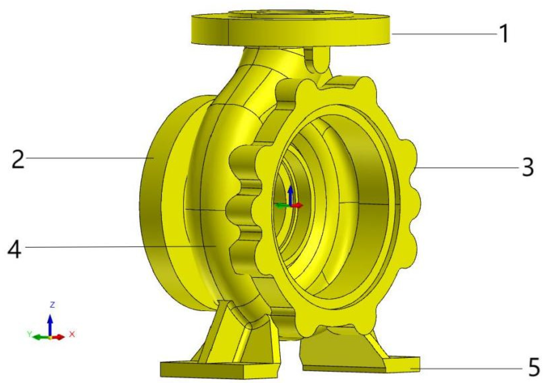
The three-dimensional solid model of the casting was created using UG NX (v12.0) software, as illustrated in Figure 1. The pump body features an inlet flange thickness of 24 mm, an outlet flange thickness of 22 mm, a volute flow passage with an arc-shaped cross-section wall thickness of 10 mm, and a base foot thickness of 12 mm. The average wall thickness is 13.57 mm, while the maximum thickness reaches 36.65 mm. This significant thickness variation, with a maximum difference of 26.65 mm, makes the casting prone to forming hot spots during the investment casting process, which can lead to defects such as hot tearing, shrinkage porosity, voids, and gas pores.

2.2. Numerical Simulation Modeling for the Titanium Alloy Pump Body Casting

The simulation of the casting process using ESI ProCAST (v2024.0) software was carried out by following the steps below. First, the initial finite element model was constructed, comprising the gating system and the casting itself, with gravity casting selected as the simulated process. After model creation, the Visual-Mesh module was used for meshing. To balance computational precision and efficiency, the mesh size was set to 3 mm in the casting region (to ensure detail resolution) and 6 mm for the riser and runners (to simplify calculation in non-critical areas). Simultaneously, the mold shell thickness was set to 10 mm. The final mesh consisted of 165,448 surface elements and 1,489,229 volume elements. The parameters for the initial scenario were as follows: pouring temperature of 1725 °C, shell preheating temperature of 400 °C, and pouring time of 7 s. Further simulation parameter settings, detailed in

Table 2. Simulation parameter settings.

Casting Material	Mold Shell Material	Interfacial Heat Transfer Coefficient	Cooling Method	Pouring Time
ZTA2	Zirconia (ZrO2)	500 W/(m2·K)	Vacuum cooling	7 s

, were also configured.

The as-cast ZTA2 titanium alloy exhibits a tensile strength of 440 MPa, a yield strength of 370 MPa, and a density of 4.505 g/cm³. Its melting temperature range is 1668~1688 °C, with a solidus temperature of 1668 °C and a liquidus temperature of 1688 °C.

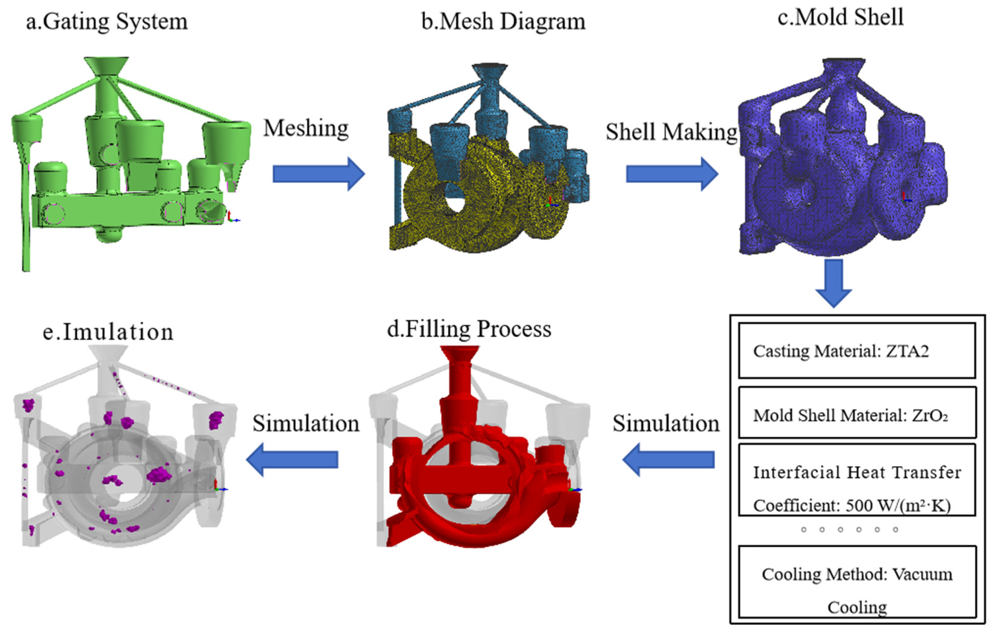
In conventional investment casting, the mold shell is primarily composed of three layers: the face coat, the intermediate coat(s), and the backup coat(s) [10]. The face coat, being the innermost layer in direct contact with the wax pattern (and subsequently the casting surface), critically determines the final surface quality of the casting. Zirconia (ZrO₂) was selected as the mold shell material [11], as zirconia shells offer low surface roughness. Specifically, ZrO₂ (stabilized with CaO) was chosen for the face coat due to its good thermodynamic stability against molten titanium alloy. The properties of the face coat material are as follows: density = 5.7 g/cm³, specific heat capacity = 1.5 J/(g·K), and thermal conductivity = 0.67 W/(m·K) [12]. The overall process flow is illustrated in Figure 2.

2.3. Analysis of Numerical Simulation Results for the Titanium Alloy Pump Body Casting

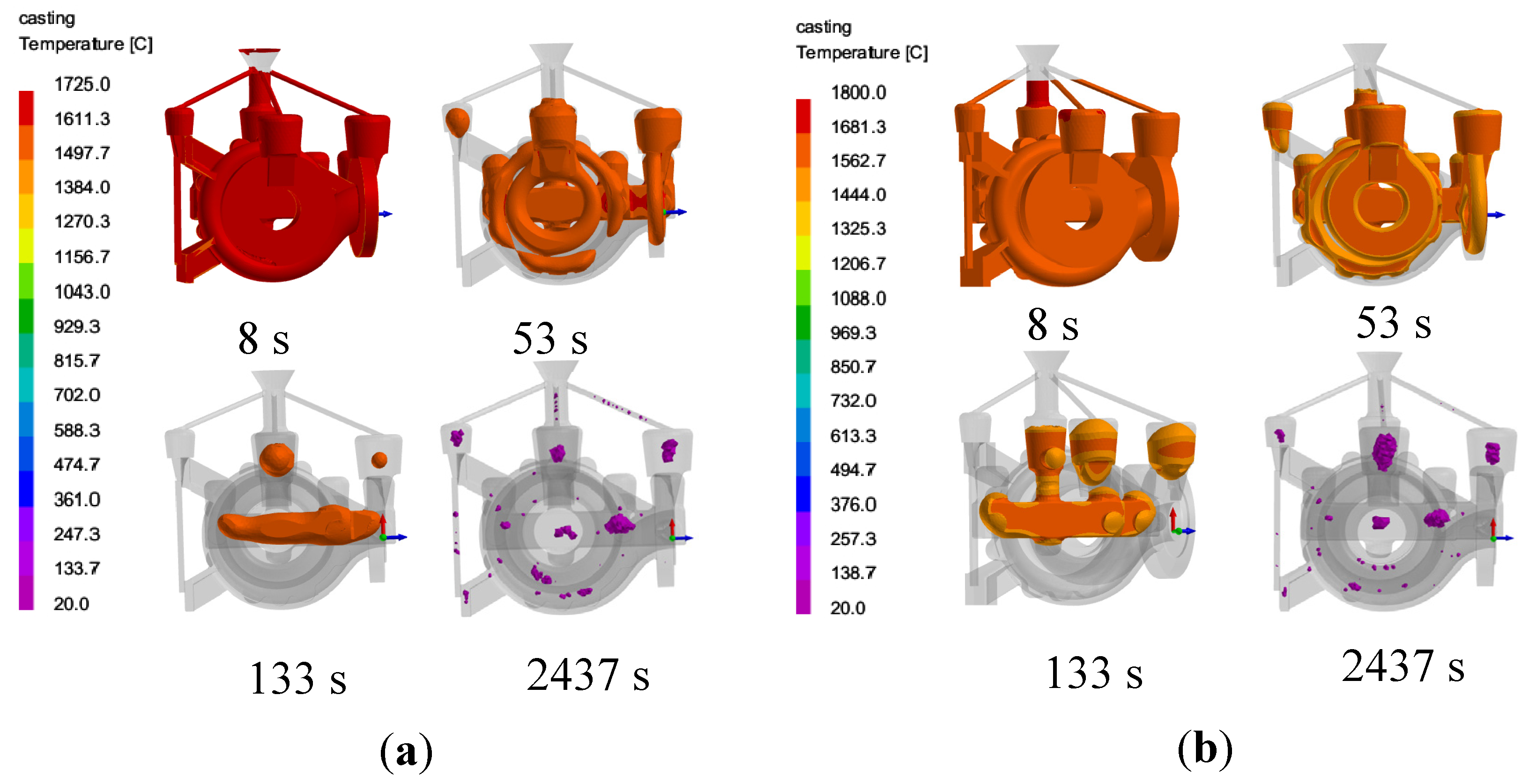
Figure 3a,b shows the simulated shrinkage evolution results for two solidification processes under different pouring temperatures and shell preheating temperatures. The display uses a cut-off criterion of >1585 °C (liquidus temperature) to identify feeding difficulty regions.

As solidification time increases, group a (Figure 3a) with lower pouring and mold temperatures begins to develop isolated liquid phase regions at 53 s. Comparing the defect predictions of the two groups reveals significant differences in both the location and volume of defects under the different pouring and shell preheating temperatures.

To further reduce casting defects, it is essential to optimize the range of process parameters. Relying solely on numerical simulation to identify the specific parameter ranges requires considerable computational time, which is not conducive to rapidly determining the optimal process window. After simulating part of the experimental data using a physical model, these data are utilized to construct a neural network model. Subsequently, the NSGA-II is employed to search for relatively optimal solutions, thereby obtaining the optimized process parameter combination for investment casting. This method holds great significance for quickly determining the range of process parameters in the production of complex castings.

3. Research on Casting Defect Prediction Modeling for the Titanium Alloy Pump Body

3.1. Process Parameters and Levels

The actual process of investment casting is highly complex, with numerous uncertain factors affecting the final casting quality [17]. Pouring temperature, pouring time, shell preheating temperature, and the wall thickness at critical sections of the casting are the primary factors influencing the solidification process [18]. To enhance the precision and efficiency of the experiment, the ranges for these key parameters in the solidification simulation were strictly determined based on actual production conditions to prevent the parameters from deviating from engineering practicality. The specific value ranges for each parameter are detailed in

Table 3. Levels of the three variables.

Pouring Temperature (°C)	Pouring Time (s)	Shell Preheating Temperature (°C)
1700–1800	3–7	400–500

. The mold shell thickness and the interfacial heat transfer coefficient were fixed at 10 mm and 500 W/(m²·K), respectively.

3.2. Orthogonal Experiment and Result Analysis

Building upon the previously optimized gating system, this study focuses on investigating the effects of three key process parameters—pouring temperature, pouring time, and shell preheating temperature—on the total defect volume and the shrinkage porosity/void volume in the TA2 titanium alloy pump body. An orthogonal experimental design method [19] was employed to plan the simulation trials, utilizing a design with three factors and five levels. The combinations of factor levels were arranged according to the L₂₅(5³) orthogonal array, as shown in

Table 4. Orthogonal experimental layout.

Group	Pouring Temperature (°C)		Pouring Time (s)		Shell Preheating Temperature (°C)		Group	Pouring Temperature (°C)		Pouring Time (s)		Shell Preheating Temperature (°C)
L1	U1	1700	V1	3	W1	400	L14	U3	1750	V4	6	W5	500
L2	U1	1700	V2	4	W3	450	L15	U3	1750	V5	7	W2	425
L3	U1	1700	V3	5	W5	500	L16	U4	1775	V1	3	W3	450
L4	U1	1700	V4	6	W2	425	L17	U4	1775	V2	4	W5	500
L5	U1	1700	V5	7	W4	475	L18	U4	1775	V3	5	W2	425
L6	U2	1725	V1	3	W5	500	L19	U4	1775	V4	6	W4	475
L7	U2	1725	V2	4	W2	425	L20	U4	1775	V5	7	W1	400
L8	U2	1725	V3	5	W4	475	L21	U5	1800	V1	3	W2	425
L9	U2	1725	V4	6	W1	400	L22	U5	1800	V3	4	W4	475
L10	U2	1725	V5	7	W3	450	L23	U5	1800	V5	5	W1	400
L11	U3	1750	V1	3	W4	475	L24	U5	1800	V4	6	W3	450
L12	U3	1750	V2	4	W1	400	L25	U5	1800	V5	7	W5	500
L13	U3	1750	V3	5	W3	450

:

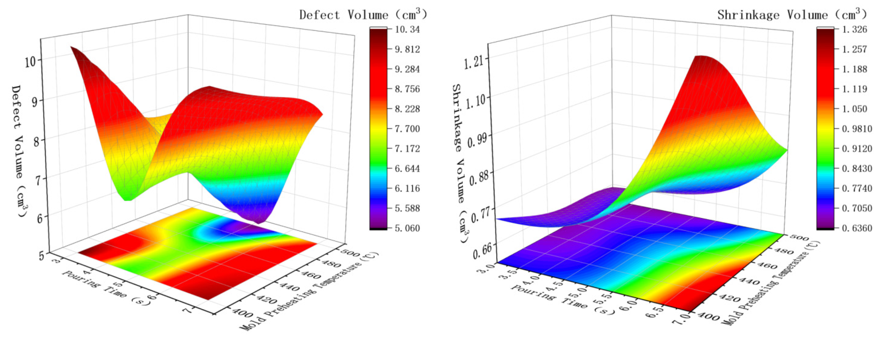
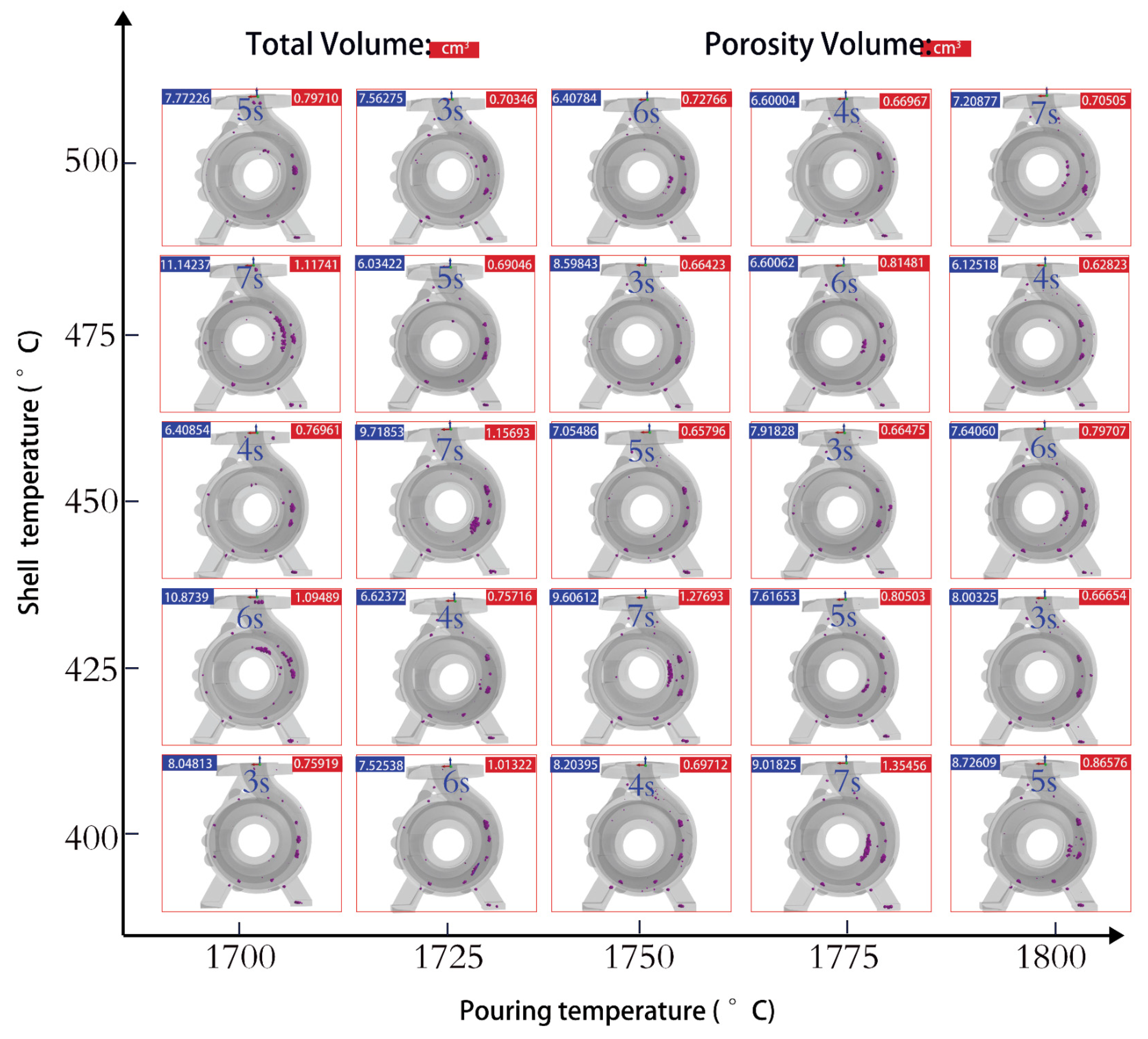
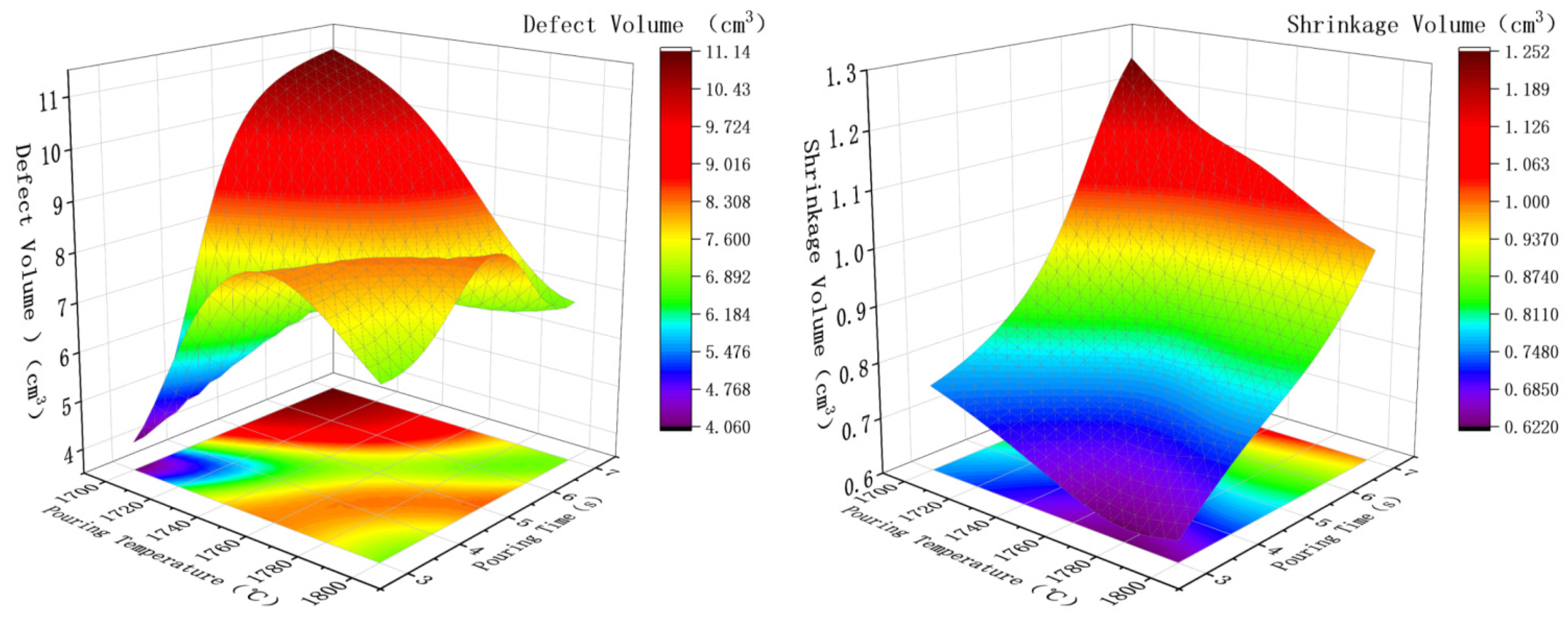
As shown in Figure 4, The defect and shrinkage porosity/void volumes were calculated by the ESI ProCAST (v2024.0) software. The results indicate that larger defects were primarily concentrated within the parameter range of a pouring temperature between 1700 °C and 1750 °C, coupled with a shell preheating temperature between 425 °C and 475 °C. Conversely, significantly smaller defect volumes were observed when the pouring temperature was between 1775 °C and 1800 °C and the shell preheating temperature was between 475 °C and 500 °C.

3.3. BP Neural Network Prediction Model Based on Particle Swarm Optimization Algorithm

3.3.1. Fundamentals of the Particle Swarm Optimization Algorithm

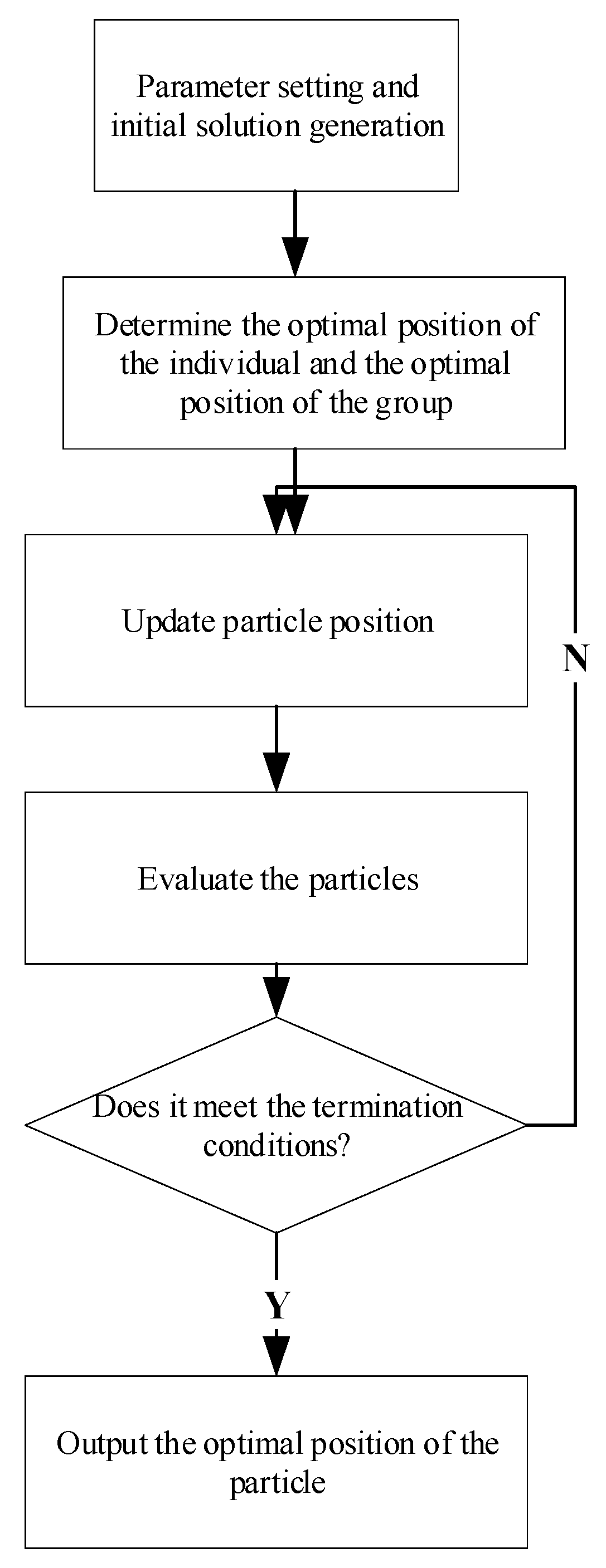
The PSO algorithm [21] is an evolutionary computation technique inspired by the study of bird flocking behavior. As an iteration-based optimization tool, it possesses both global search capabilities and strong local search ability [22]. The PSO algorithm has demonstrated excellent performance in solving both continuous and discrete optimization problems due to its simple structure, ease of implementation, lack of a requirement for gradient information, and few parameters to adjust. Notably, its inherent real-number coding characteristic makes it particularly suitable for handling real-value optimization problems. In recent years, PSO has become a prominent research topic in the field of international intelligent optimization. The operational flowchart of the Standard Particle Swarm Optimization (SPSO) algorithm is illustrated in Figure 5.

Input: Number of input layer nodes, number of hidden layer nodes, number of output layer nodes; number of iterations; population size; c1, c2; step size

Output: Optimal weights w, thresholds b

Step 1: Initialize the particle swarm

Step 2: For each particle, calculate the prediction error (MSE) of the corresponding BP model as its fitness value

Step 3: Record the personal best fitness (pbest) of each particle and the global best fitness (gbest) of the population

Step 4: For t = 1 to 100:

a. For each particle, update velocity: $${\mathrm{v}}_{\mathrm{i}}=\mathrm{w}\times {\mathrm{v}}_{\mathrm{i}}+\mathrm{c}1\times \mathrm{r}\mathrm{a}\mathrm{n}\mathrm{d}\left(\right)\times (\mathrm{p}\mathrm{b}\mathrm{e}\mathrm{s}{\mathrm{t}}_{\mathrm{i}}-{\mathrm{x}}_{\mathrm{i}})+\mathrm{c}2\times \mathrm{r}\mathrm{a}\mathrm{n}\mathrm{d}\left(\right)\times (\mathrm{g}\mathrm{b}\mathrm{e}\mathrm{s}\mathrm{t}-{\mathrm{x}}_{\mathrm{i}})$$

b. Update position: ${\mathrm{x}}_{\mathrm{i}}={\mathrm{x}}_{\mathrm{i}}+0.2\times {\mathrm{v}}_{\mathrm{i}}(\mathrm{r}\mathrm{e}\mathrm{s}\mathrm{t}\mathrm{r}\mathrm{i}\mathrm{c}\mathrm{t}{\mathrm{x}}_{\mathrm{i}}\in [-\mathrm{1,1}\left]\right)$

c. Calculate the new fitness value, and update pbest and gbest

Step 5: Output the weights w and thresholds b corresponding to gbest

The Particle Swarm Optimization algorithm exhibits prominent advantages in solving multi-objective optimization problems, which are mainly reflected in the following aspects. First, the algorithm itself possesses efficient search capabilities [23], facilitating the exploration of optimal solutions within multi-objective scenarios. Second, it can conduct parallel searches for multiple non-dominated solutions in the form of a population, thereby obtaining a set of Pareto-optimal solutions. Furthermore, the algorithm demonstrates good generality; it is not only suitable for handling various types of objective functions and constraints but can also be easily integrated with traditional optimization methods. This integration helps overcome its own limitations and leads to more efficient problem-solving. Consequently, applying the PSO algorithm to multi-objective optimization problems holds considerable potential and advantages.

3.3.2. Fundamentals of the BP Neural Network

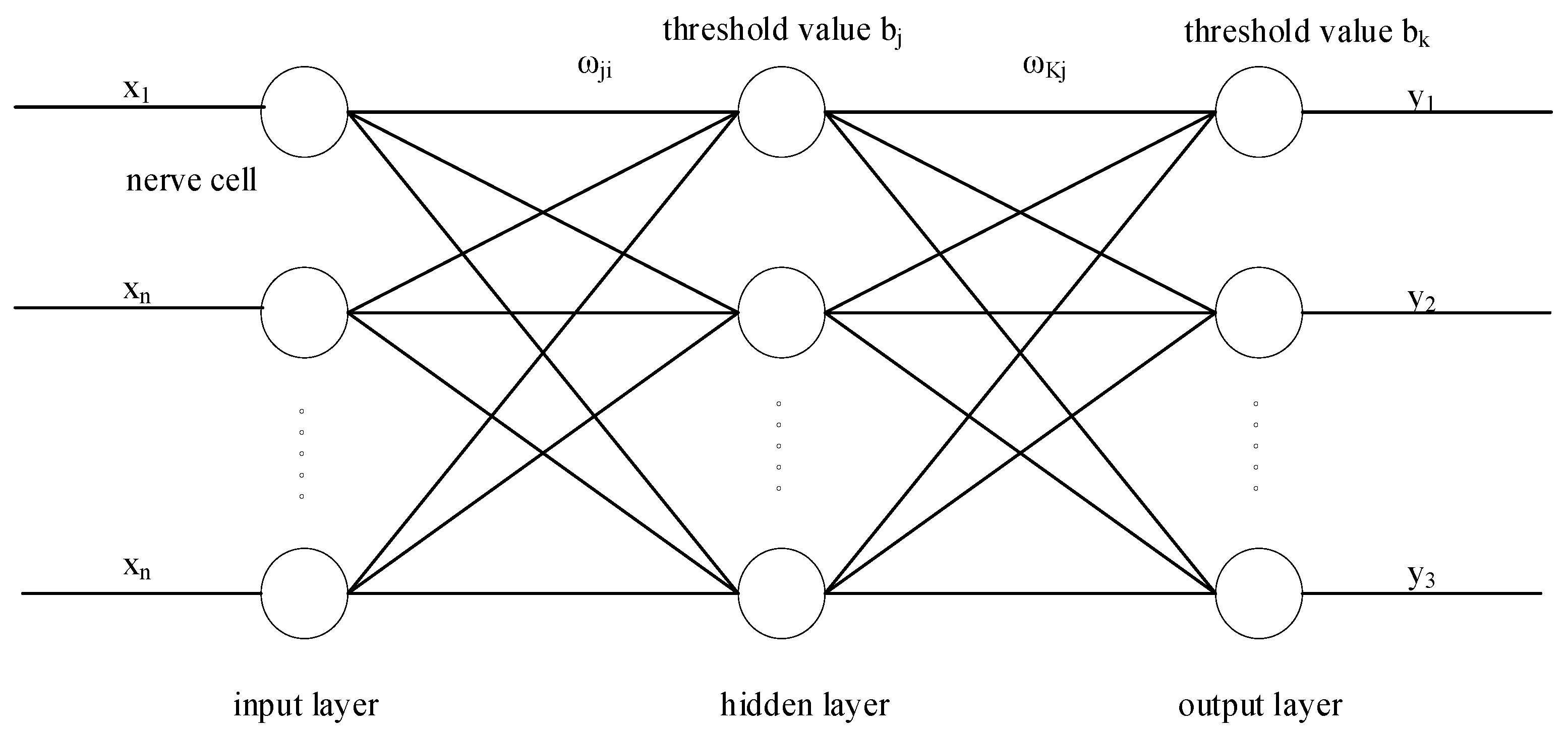
A BP neural network consists of three layers: an input layer, one or more hidden layers, and an output layer [24]. Each layer contains multiple neurons, with each neuron possessing a unique threshold (bias). Neurons between different layers are interconnected via weights. The number of hidden layers can be manually selected to allow the network to achieve optimal performance, as illustrated in Figure 6.

The core process of a BP neural network is training. First, the input feature data is mapped to the hidden layer(s), which then further maps it to the output layer, resulting in a predicted output value. This predicted value is then compared with the actual target value to calculate the error. Subsequently, this error is propagated backward through the network to iteratively adjust the inter-layer weights and the threshold (bias) of each neuron. This process repeats iteratively until the error meets a pre-defined requirement or the number of iterations reaches a pre-set limit, at which point the training stops. Theoretical studies have shown that a neural network can approximate any nonlinear function arbitrarily well as long as its hidden layer(s) contain a sufficient number of neurons. Due to its simple structure and strong learning capability, the BP neural network is widely applied in fields such as pattern recognition and distributed information processing.

3.3.3. Defect Prediction Model for Titanium Alloy Pump Body Casting Based on PSO-BP Neural Network

The BP neural network is a multi-layer feedforward network that employs error backpropagation. It is widely used in practical applications due to its simple structure and strong operability [25], making it particularly suitable for modeling the complex relationship between investment casting process parameters and casting defects.

However, for the small-sample, high-nonlinearity casting defect prediction scenario in this study, the standard BP neural network has prominent limitations: it is extremely sensitive to initial parameters such as weights and thresholds. After the network structure is determined, randomly initializing weights and thresholds for model training will cause the network to easily fall into local optima during the gradient descent process, resulting in large prediction deviations and poor generalization performance on unseen data. To address this targeted pain point, the PSO algorithm with excellent global search capability is introduced to adjust and optimize the initial weights and thresholds of the BP neural network before formal training. Through the global iterative search of the particle swarm, the optimal initial parameter combination that minimizes the network prediction error is obtained, which fundamentally mitigates the randomness of initial parameter setting in the traditional BP model, and significantly improves the learning efficiency, prediction precision and generalization stability of the network in this defect prediction task [26,27].

In this study, three key investment casting process parameters (pouring temperature, pouring time, and shell preheating temperature) that have a significant impact on casting defects are determined as the input variables of the network, while the two core defect quality indicators (total casting defect volume and shrinkage porosity/void volume) are set as the output variables of two independent prediction models, respectively. Correspondingly, the input layer of each BP neural network is set to 3 nodes matching the number of input process parameters, and the output layer is set to 1 node corresponding to a single defect indicator. For the training algorithm of the network, the Levenberg–Marquardt (LM) algorithm is selected: on the one hand, it has the advantages of fast convergence speed and high solution precision for medium-scale nonlinear regression tasks matching this study; on the other hand, it can be well compatible with the initial weights and thresholds optimized by the PSO algorithm, ensuring the stability and efficiency of the subsequent network training process.

The Inputs of the paper are 3 key parameters (pouring temperature, pouring time, and shell preheating temperature), and a combination of “L₂₅(5³) orthogonal experiment + 97 sets of random samples” is adopted. The orthogonal experiment (25 sets) has uniformly covered 5 levels of the 3 parameters, ensuring the representativeness of the parameter space (without missing key combinations). The 97 sets of random samples fill the “parameter gaps” not covered by the orthogonal experiment, enabling the dataset to cover the complete parameter domain.

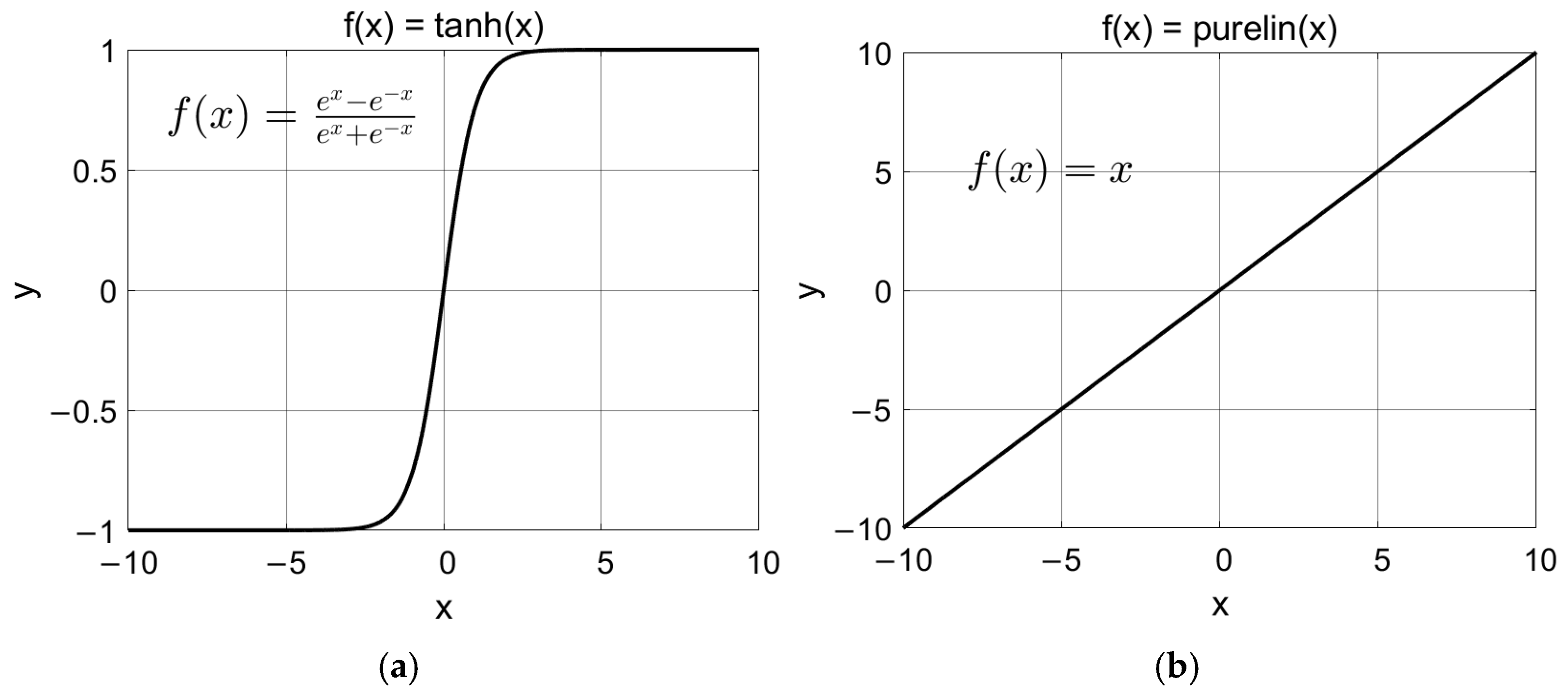
Regarding the activation functions, as shown in Figure 7, the hyperbolic tangent sigmoid function (tansig) is used for the hidden layer, and a linear function (purelin) is adopted for the output layer, which is appropriate for regression problems.

The essence of neural network training lies in continuously adjusting the weights and thresholds to gradually reduce the network’s output error [28]. In this study, the Particle Swarm Optimization (PSO) algorithm is employed to optimize the initial weights and thresholds of the BP neural network. This approach aims to identify the optimal initial parameters, thereby mitigating the local optima problem often encountered in traditional BP networks due to random parameter initialization.

To accurately match the requirements of the defect prediction scenario for titanium alloy pump body castings, it is necessary to determine the parameter range and implementation logic of sensitivity analysis around the nonlinear mapping characteristics of “process parameters–defect volume”. Through quantitative analysis, optimal parameter combinations are screened to ultimately ensure the prediction precision and robustness of the model in actual production scenarios.

3.3.4. Single-Factor Sensitivity Analysis of Model Hyperparameters

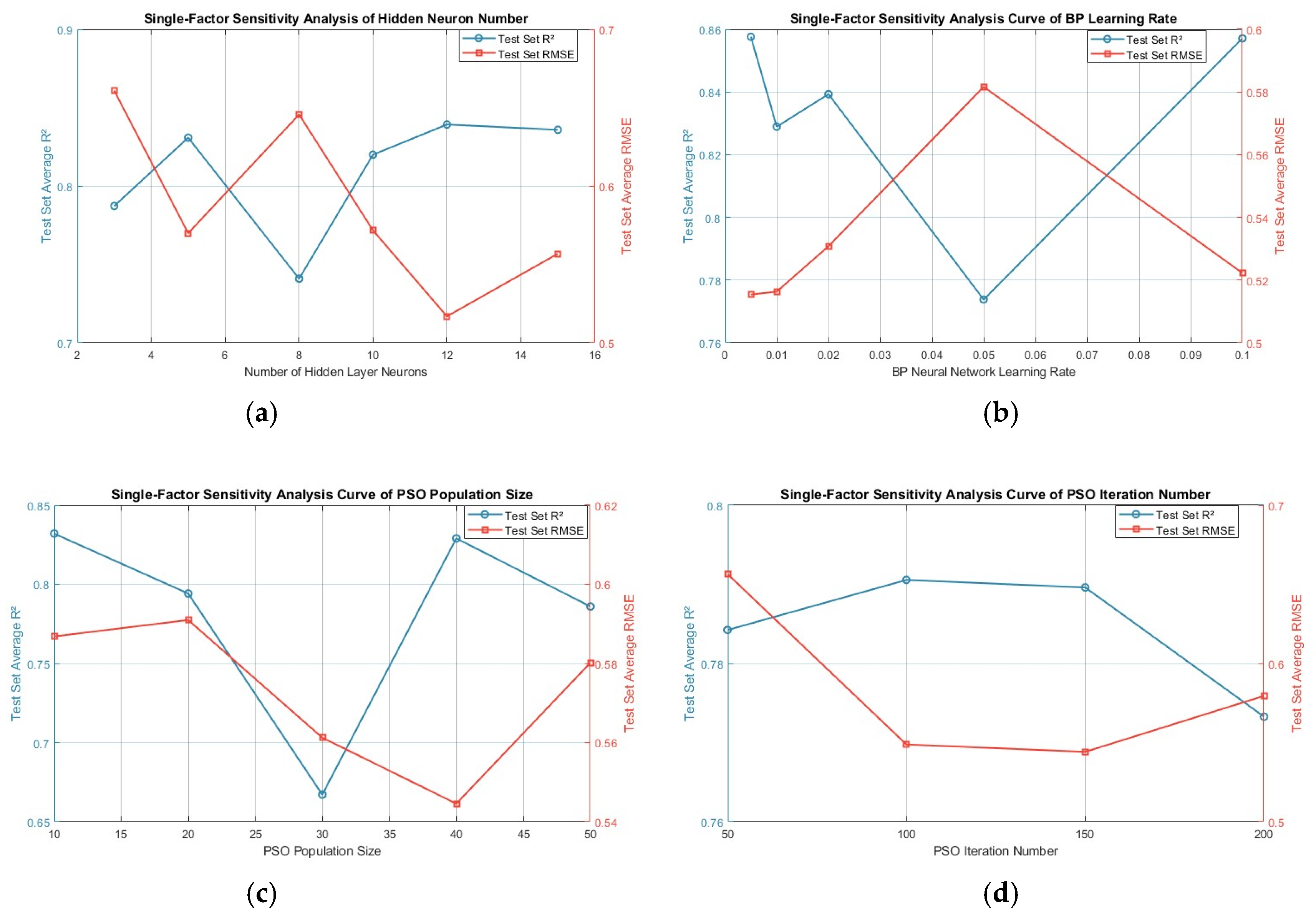
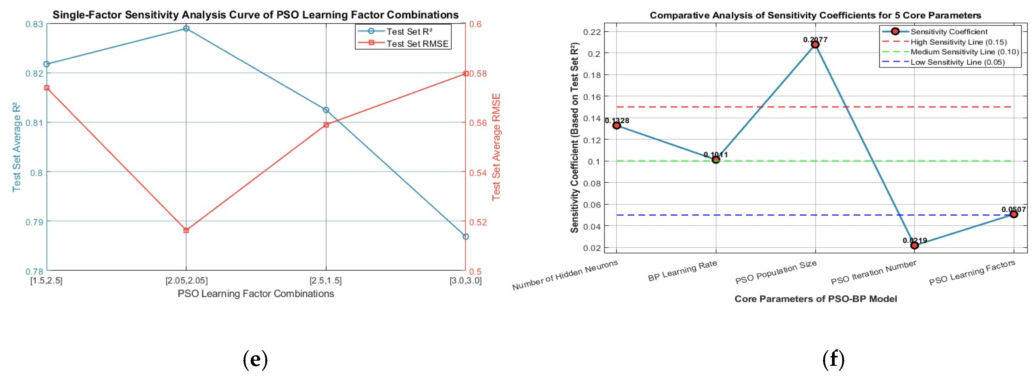
Combined with the actual needs of defect prediction for titanium alloy pump body castings, the influences of various parameters on model performance exhibit significant hierarchical differences, as shown in Figure 8:

Based on the sensitivity coefficient classification criteria, the model’s sensitive parameters can be divided into three levels: high, medium, and low. Among them, the high-sensitive parameter is the PSO population size (0.2077) with a sensitivity coefficient > 0.15, which has the most significant impact on the model’s prediction performance. A slight change in this parameter can trigger drastic fluctuations in the model’s fitting degree and prediction performance. When the PSO population size increases from 10 to 30, the coefficient of determination (R²) of the test set plummets from 0.8321 to 0.6671, and the root mean square error (RMSE) fluctuates slightly from 0.5868 to 0.5612. During this stage, the excessive increase in population size leads to redundant particle optimization and premature algorithm convergence, resulting in a significant decline in the model’s fitting precision for the input-output mapping relationship and falling into the local optimal trap. However, when the population size increases from 30 to 40, the R² rebounds strongly to 0.8291, and the RMSE drops to the lowest level of 0.5446 in the entire interval, with optimization precision and fitting effect reaching their peaks simultaneously. When the population size exceeds 40, the R² falls back to 0.7860, the model performance continues to deteriorate, and the computational load increases significantly. Considering the fitting effect, optimization precision, and computational efficiency comprehensively, a population size of 40 is determined as the optimal value to achieve “sufficient global optimization–controllable computational cost–avoidance of local optima”.

The medium-sensitive parameters are the number of hidden neurons (0.1328) and the BP learning rate (0.1011) with sensitivity coefficients between 0.10 and 0.15. The rationality of their values directly affects the neural network’s fitting ability, convergence stability, and predictive power. Changes in these parameters have a noticeable impact on model performance but no risk of drastic failure.

When the number of neurons increases from 3 to 5, the coefficient of determination (R²) of the test set rises from 0.7872 to 0.8309, and the root mean square error (RMSE) decreases from 0.6608 to 0.5699. The increase in the number of neurons effectively expands the nonlinear mapping capability of the network and significantly improves the fitting precision of the model. When the number of neurons increases from 5 to 8, the R² drops to the lowest value of 0.7409 in the entire interval, and the imbalanced network structure leads to a phased deterioration of the fitting ability. When the number of neurons continues to increase from 8 to 12, the R² climbs to the maximum value of 0.8393, and the RMSE drops to the lowest value of 0.5168, with the fitting and prediction performance of the model reaching the optimal level. Beyond 12, the increase in R² is less than 0.005, the decrease in RMSE tends to level off, the improvement in model performance saturates, and there is a risk of redundant overfitting. Considering the nonlinear fitting ability, anti-overfitting characteristics and computational efficiency comprehensively: although increasing the number of neurons from 5 to 12 can slightly improve the fitting precision (R² only increases by 0.0084), it will significantly increase the number of network parameters and training time (doubling the number of neurons leads to an increase in computational load of about 60%). When the number of neurons is 5, it can already meet the fitting precision required for engineering applications (R² = 0.8309, RMSE = 0.5699), with optimal computational efficiency and no risk of overfitting. Therefore, the optimal number of hidden neurons is determined to be 5.

For the BP learning rate: when the learning rate increases from 0.005 to 0.050, the test set R² continues to plummet from 0.8576 to 0.7738, and the RMSE rises from 0.5154 to 0.5816. A medium learning rate causes imbalanced network gradient updates, resulting in prediction oscillations in critical intervals and a significant decline in convergence stability. When the learning rate adjusts back from 0.050 to 0.100, the R² rebounds strongly to 0.8571, returning to the optimal level. When the learning rate is 0.005, the R² reaches the highest value among all parameters, and the RMSE is the lowest in the entire interval, with the model converging stably without oscillations and achieving the optimal prediction precision. Therefore, the optimal BP learning rate is determined to be 0.005.

The low-sensitive parameters are the PSO learning factors (0.0507) and PSO number of iterations (0.0219) with sensitivity coefficients < 0.10. Different values of these parameters have a weak impact on model performance. Under parameter fluctuations, the model’s fitting degree and error remain highly stable, with limited adjustable space and optimization potential.

The optimization results of the PSO number of iterations show that when the number of iterations increases from 50 to 100, the test set R² rises slightly from 0.7842 to 0.7906, and the RMSE decreases from 0.6565 to 0.5488. The increase in the number of iterations enables the particle swarm to fully converge, providing better initial weights for the BP network. When the number of iterations is in the range of 100~150, the R² and RMSE hardly change, the curve tends to level off, the fitness converges completely, and the performance reaches a saturated and stable state. When the number of iterations exceeds 150 and increases to 200, the R² decreases slightly to 0.7733, and the RMSE rises back to 0.5795. Excessive iterations cause redundant oscillations of the algorithm, resulting in slight performance degradation and waste of computational resources. Therefore, 100 iterations are selected as the optimal PSO number of iterations.

Based on the studies by Clerc M, Wang Dongfeng et al. [29,30], four different combinations of particle swarm learning factors were set up for testing. The test results show that the fluctuation range of the R² value on the test set corresponding to different parameter combinations is only 0.0420, indicating negligible differences in model performance. Among them, the balanced cognitive and social learning factor combination [2.05, 2.05] achieves the best performance, with a corresponding R² of 0.8289 and a Root Mean Square Error (RMSE) as low as 0.5163. The combination [1.50, 2.50] focusing on social learning and the combination [2.50, 1.50] focusing on individual cognitive learning achieve R² values of 0.8217 and 0.8125, respectively, with performance close to that of the optimal combination. The [3.0, 3.0] combination with excessively large dual learning factors yields the worst performance, with its corresponding R² dropping to 0.7869. The balanced combination can reconcile the global exploration and local exploitation capabilities of the algorithm, thus achieving optimal stability.

4. Determination of the Optimal Model and Performance Verification

4.1. Establishment of the Defect Prediction Model

Based on the principle of “priority optimization of high-sensitive parameters and efficiency balance of medium and low-sensitive parameters”, combined with the actual needs of defect prediction for titanium alloy pump body castings, the optimal combination of network structure hyperparameters and PSO parameters is determined through single-factor sensitivity analysis, as shown in

Table 5. Parameter Values of the PSO-BP Neural Network Model.

Parameter Category	Parameter Values
Network Structure	Number of Hidden Neurons = 5
BP Training Parameters	Learning Rate = 0.005
PSO Parameters	Population Size = 40, Number of Iterations = 100, Learning Factors = [2.05, 2.05]

. After substituting the optimal initial parameters optimized by the PSO algorithm into the BP neural network, the trainbr function (Bayesian Regularization Training Algorithm) is adopted for the formal training of the network. This training algorithm can constrain the network complexity by introducing a regularization term into the loss function, which forms a dual optimization mechanism with the PSO-based initial parameter optimization: PSO optimization solves the local optimum problem in the training process, while Bayesian regularization suppresses the overfitting risk of the model, so as to further improve the generalization performance of the model on the small-sample dataset in this study.

Substitute this parameter combination into the model. The training function of the BP network in the code adopts trainbr (Bayesian Regularization Training Algorithm). This algorithm constrains the network complexity by introducing a regularization term into the loss function. Based on the Bayesian framework, it treats network weights as random variables, estimates the weights by maximizing the posterior probability, and automatically balances the training error and network complexity. It effectively suppresses overfitting and improves the model’s generalization ability on the test set, especially suitable for small-sample datasets.

Meanwhile, to objectively evaluate the model’s generalization performance, the code introduces 5-Fold Cross Validation. The dataset is randomly divided into K mutually exclusive subsets. One subset is sequentially selected as the test set, and the remaining K-1 subsets serve as the training set. K rounds of training and testing are completed in a loop. By averaging the K evaluation indicators, the randomness caused by a single dataset division is eliminated, ensuring the reliability of the model performance evaluation.

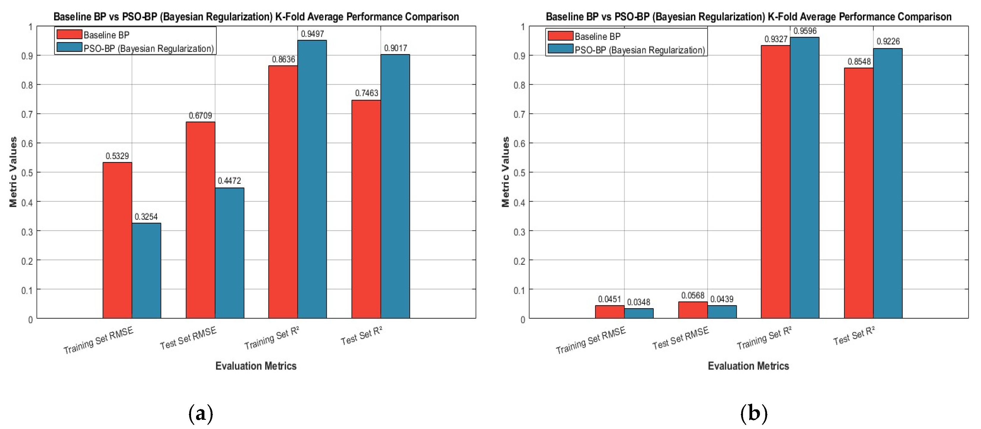
As shown in Figure 9, the two bar charts compare the prediction performance of the basic BP neural network and the PSO-BP (Bayesian Regularization) neural network for total defect volume (left chart) and shrinkage porosity/void volume (right chart) under 5-fold cross-validation. Using two core indicators—root mean square error (RMSE) and coefficient of determination (R²)—they quantitatively verify the generalizable improvement effect of the dual strategy of “PSO weight optimization + Bayesian regularization” in the two types of defect volume prediction tasks.

For the prediction of total defect volume (left chart): In terms of RMSE, the RMSE of the basic BP neural network on the training set is 0.5329, while that of the PSO-BP neural network decreases to 0.3254 (a decrease of 38.94%), indicating that PSO of initial weights can effectively avoid local optima. The RMSE on the test set decreases from 0.6709 to 0.4472 (a decrease of 33.34%), verifying that Bayesian regularization can suppress overfitting and improve the generalization stability of the model. In terms of R², the R² on the training set increases from 0.8636 to 0.9497 (an increase of 9.97%), and the R² on the test set jumps from 0.7463 to 0.9017 (an increase of 20.82%), proving that the generalization ability of PSO-BP is significantly superior to that of the basic BP, solving the overfitting problem.

For the prediction of shrinkage porosity/void volume (right chart): The RMSE on the training set decreases from 0.0451 to 0.0348 (a decrease of 22.84%), and the RMSE on the test set decreases from 0.0568 to 0.0439 (a decrease of 22.71%); the R² on the training set increases from 0.9327 to 0.9596 (an increase of 2.88%), and the R² on the test set jumps from 0.8548 to 0.9226 (an increase of 7.93%). This result indicates that the dual mechanism of “PSO weight optimization + Bayesian regularization” has cross-task generalizability and is not an accidental improvement in a single task.

In summary, whether for the prediction of total defect volume or shrinkage porosity/void volume, the PSO-BP (Bayesian Regularization) neural network, through the dual mechanism of “weight optimization to suppress local optima + regularization to suppress overfitting”, outperforms the basic BP in prediction precision (reduced RMSE) and generalization ability (improved R²). This verifies the effectiveness, generalizability, and practicality of the optimization strategy, providing a reliable improved solution for solving complex nonlinear prediction problems such as casting defects.

4.2. Performance Verification of the Defect Prediction Model

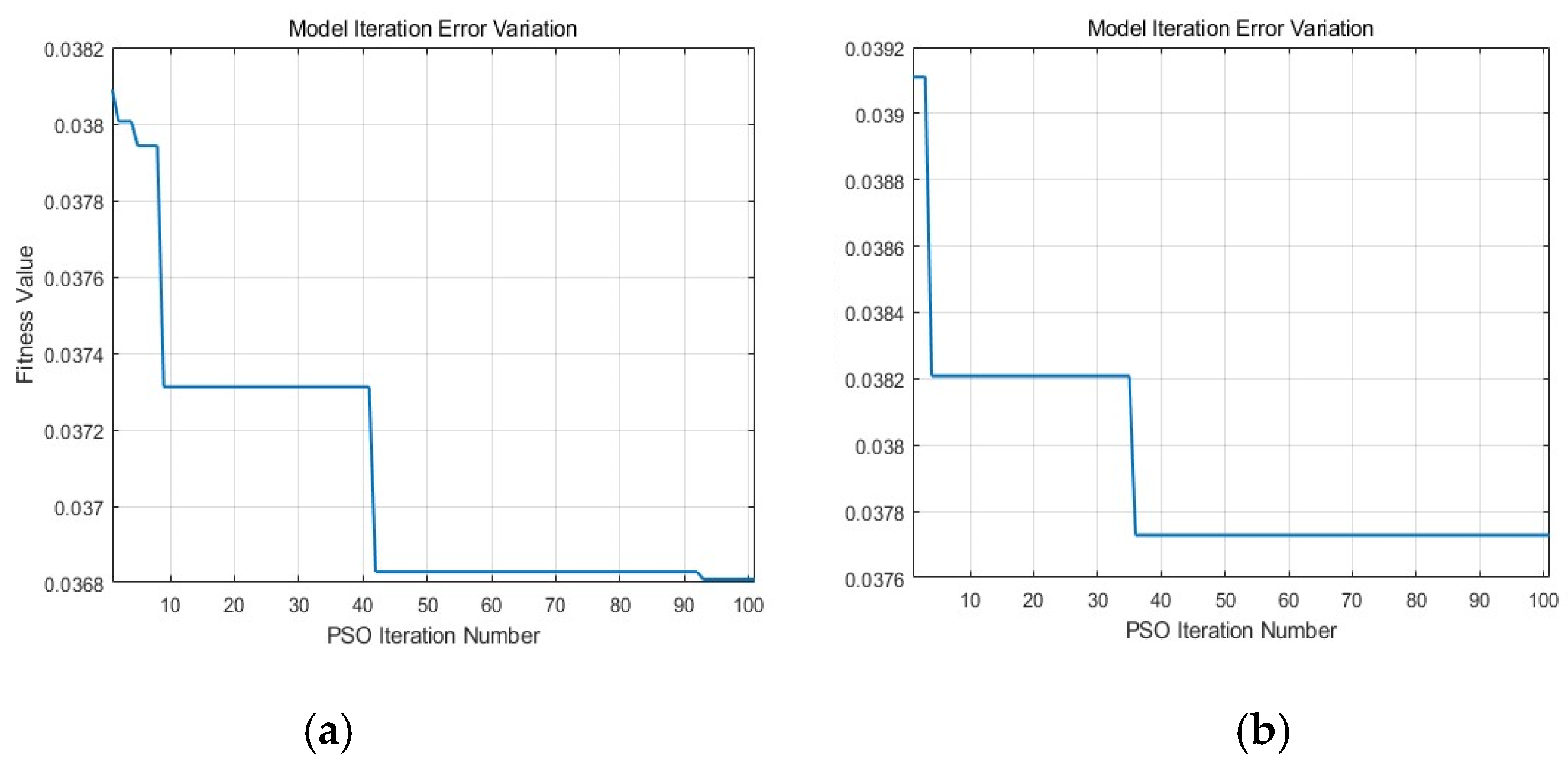
In this study, the constructed PSO-BP neural network takes three process parameters of investment casting—pouring temperature, shell preheating temperature, and pouring time—as inputs, and the total defect volume and shrinkage porosity/void volume of castings as the outputs of the two models respectively (with 3 nodes in the input layer and 1 node in the output layer). The Levenberg–Marquardt (LM) algorithm, which features fast convergence and small mean square error, is selected as the training algorithm. The dataset combines an L₂₅(5³) orthogonal experiment (25 groups) and 97 random samples to cover the complete parameter domain. For activation functions, the hyperbolic tangent sigmoid function (tansig) is adopted in the hidden layer and the linear function (purelin) in the output layer, which is suitable for regression problems. The optimal parameter configuration is determined as follows: 5 hidden neurons, a BP training learning rate of 0.005, and PSO parameters including a population size of 40, 100 iterations, and learning factors of [2.05, 2.05]. The fitness curves of the two models are shown in Figure 10 below:

The fitness curves in both figures show a continuous downward trend and gradually stabilize, gradually converging from an initial value of approximately 0.0382 to about 0.0368. This indicates that the particle swarm optimization algorithm continuously approaches the optimal solution during iterations without divergence or oscillation, which conforms to the normal convergence characteristics of the PSO algorithm.

In the early stage (the first 10 iterations), the fitness value decreases rapidly, indicating that the algorithm can efficiently explore the solution space and quickly locate the better region at the initial stage. In the middle stage (20–40 iterations), it decreases again after a plateau, showing that the algorithm can still continue to optimize after a certain degree of exploration, and finally enters a stable state after about 50 iterations.

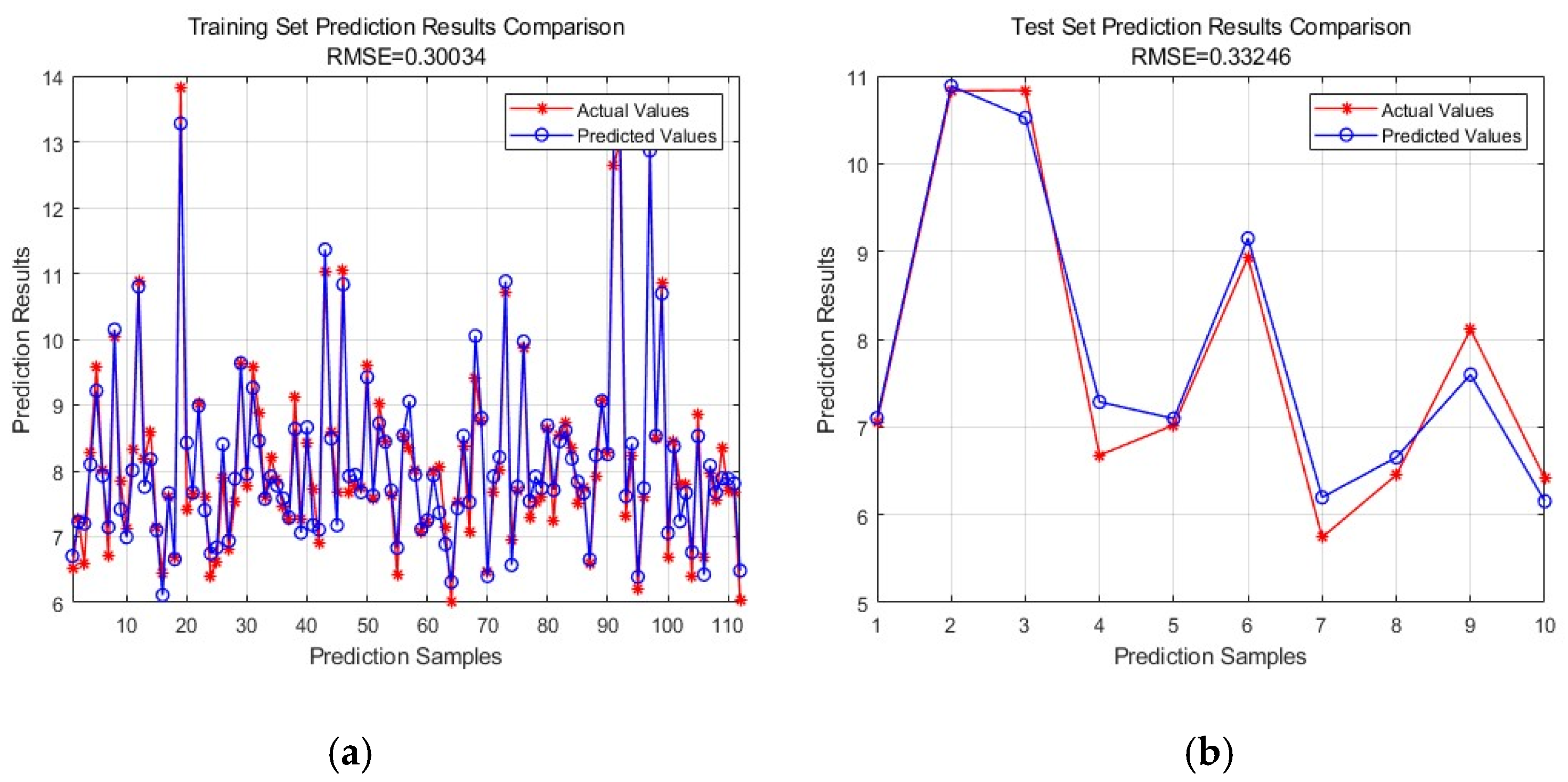
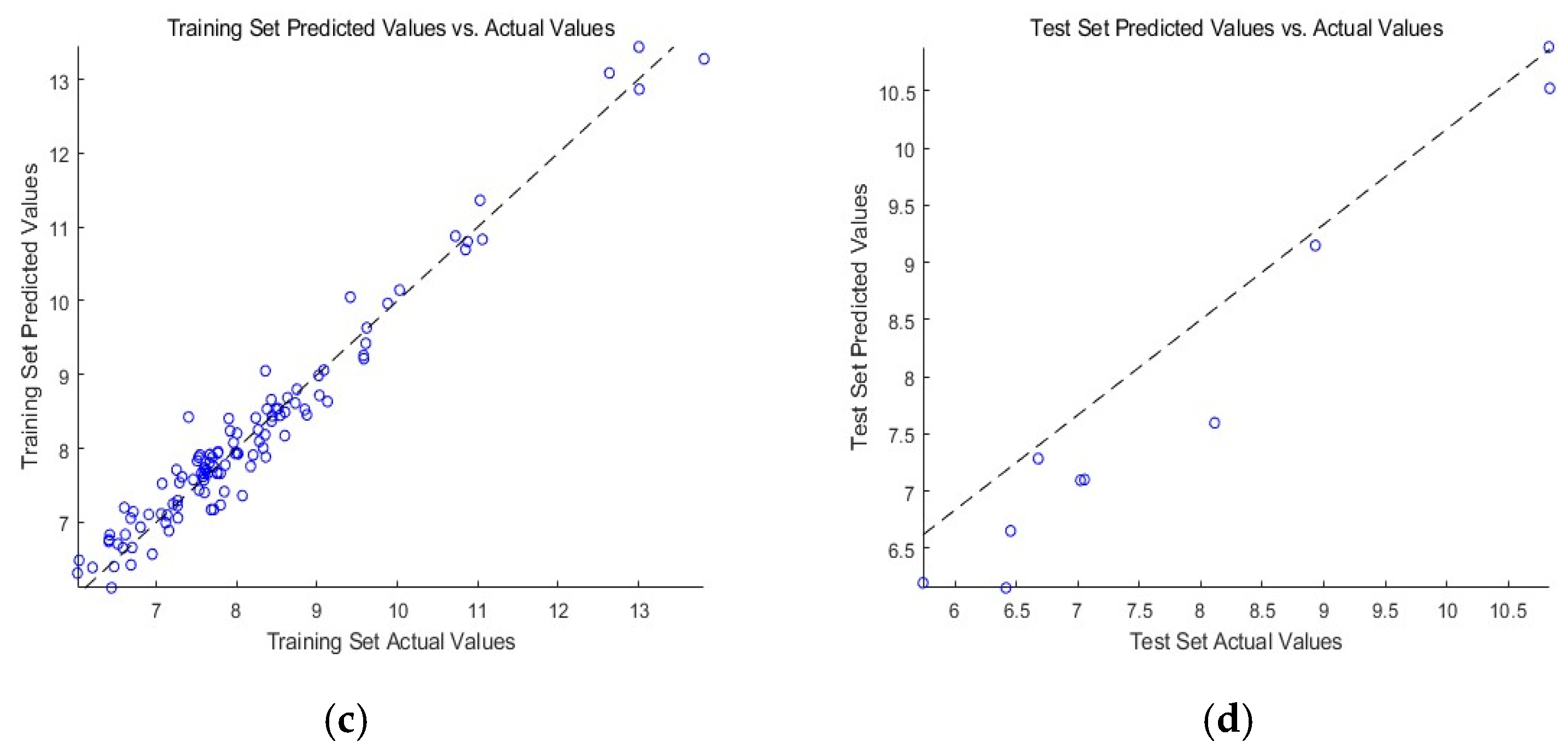
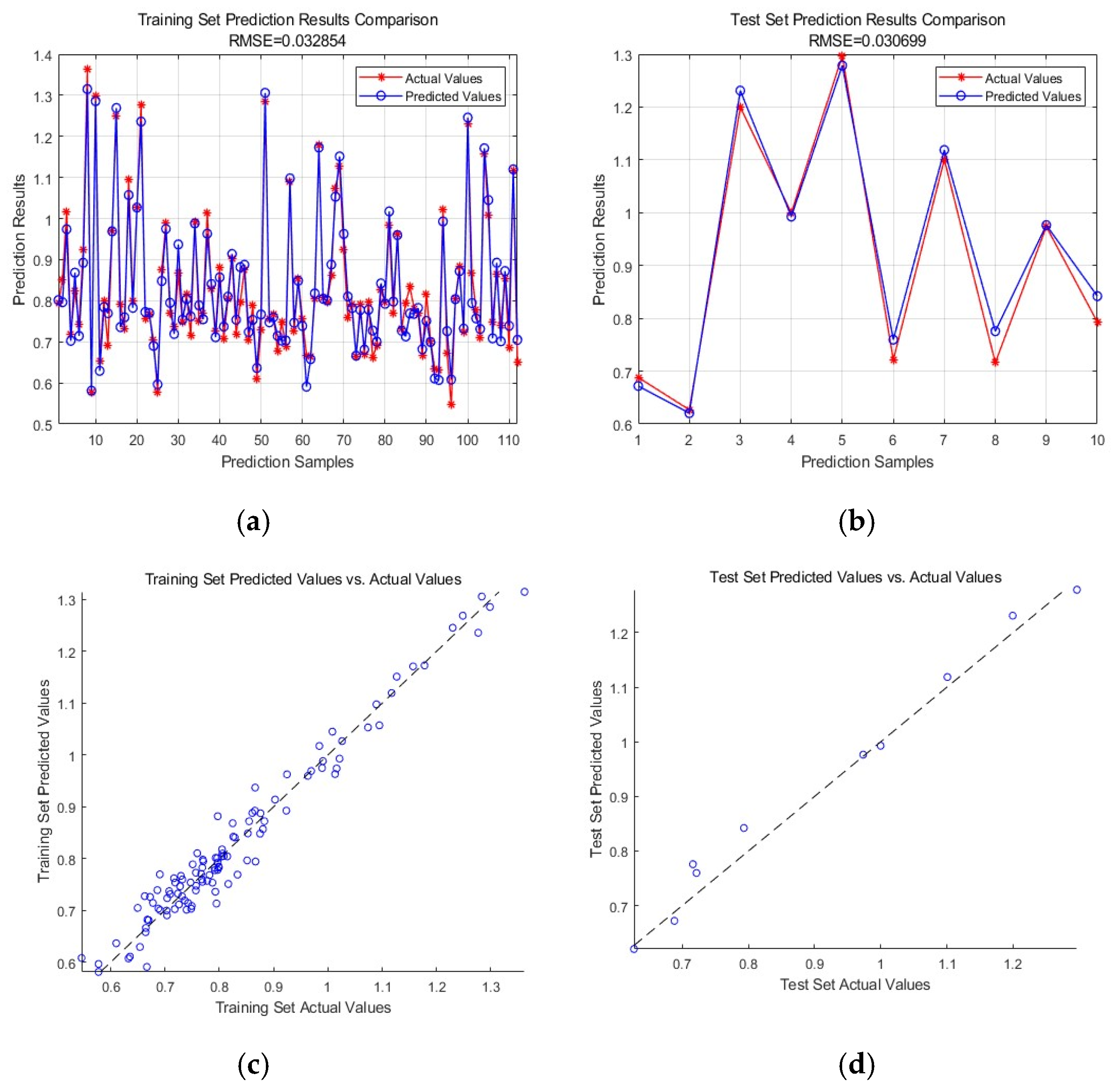
The comparison of the fitting effect and prediction performance between the prediction models for total defect volume and shrinkage porosity/void volume is shown in Figure 11 and Figure 12.

According to the prediction results of shrinkage porosity/void volume, the prediction curves of the model in the training set and test set are highly consistent with the fluctuation trend of actual values, without obvious deviation, jump or lag. The RMSE of the training set is as low as 0.03854 and that of the test set is 0.03369, both of which are at a very low level with a slight difference, indicating strong stability of the model in iterative prediction. From the scatter fitting plots, the samples of shrinkage porosity/void volume are closely clustered on both sides of the fitting diagonal with low dispersion, showing a strong linear positive correlation between predicted and actual values, which fully proves that the model can accurately capture the nonlinear correlation between investment casting process parameters and shrinkage porosity/void volume.

Comprehensively combined with the chart results of total defect volume and shrinkage porosity/void volume prediction, the PSO-BP model shows excellent performance in both types of casting defect prediction scenarios. In terms of prediction trend fitting, the prediction curves of the training and test sets can synchronously match the variation trend of actual values with high fitting degree. In terms of numerical error control, the RMSE values of the training and test sets for both tasks are maintained in a low range without significant difference, avoiding overfitting, underfitting, divergence and oscillation. In terms of scatter fitting effect, the samples of total defect volume and shrinkage porosity/void volume are densely distributed near the fitting diagonal without a large number of discrete outliers, and the model achieves high goodness of fit and prediction consistency.

As can be seen from

Table 6. Evaluation of the neural network model.

Evaluation	PSO-BP Total Defect Volume	PSO-BP Shrinkage Porosity/Shrinkage Void Volume
Training Set R2	0.95613	0.96158
Validation Set R2	0.96333	0.98108
Validation Set RMSE	0.33246	0.0307
Validation Set MSE	0.11053	0.00094
Validation Set MAPE	3.8101%	2.9847%
Validation Set MAE	0.2746	0.02047

, for the prediction of total defect volume and shrinkage porosity/shrinkage void volume, the PSO-BP model achieves validation set R² values of 0.96333 and 0.98108, respectively, indicating an excellent fitting effect, with validation set MAPE values controlled at 3.8101% and 2.9847%, respectively, and all error indicators remaining at a low level. Moreover, no significant difference exists between the performance of the training set and the validation set, demonstrating that the model has no overfitting problem and its generalization ability and prediction precision can meet the practical requirements of quantitative prediction of casting defects.

In conclusion, the constructed PSO-BP model features high-precision fitting capability and strong generalization performance. It can realize stable and accurate quantitative prediction of the two core defect indexes (total casting defect volume and shrinkage porosity/shrinkage void volume), making it well applicable to the prediction of various types of defects in investment casting with outstanding universality and engineering practical value.

5. Factors Influencing Casting Defects in the Titanium Alloy Pump Body

5.1. SHAP Analysis

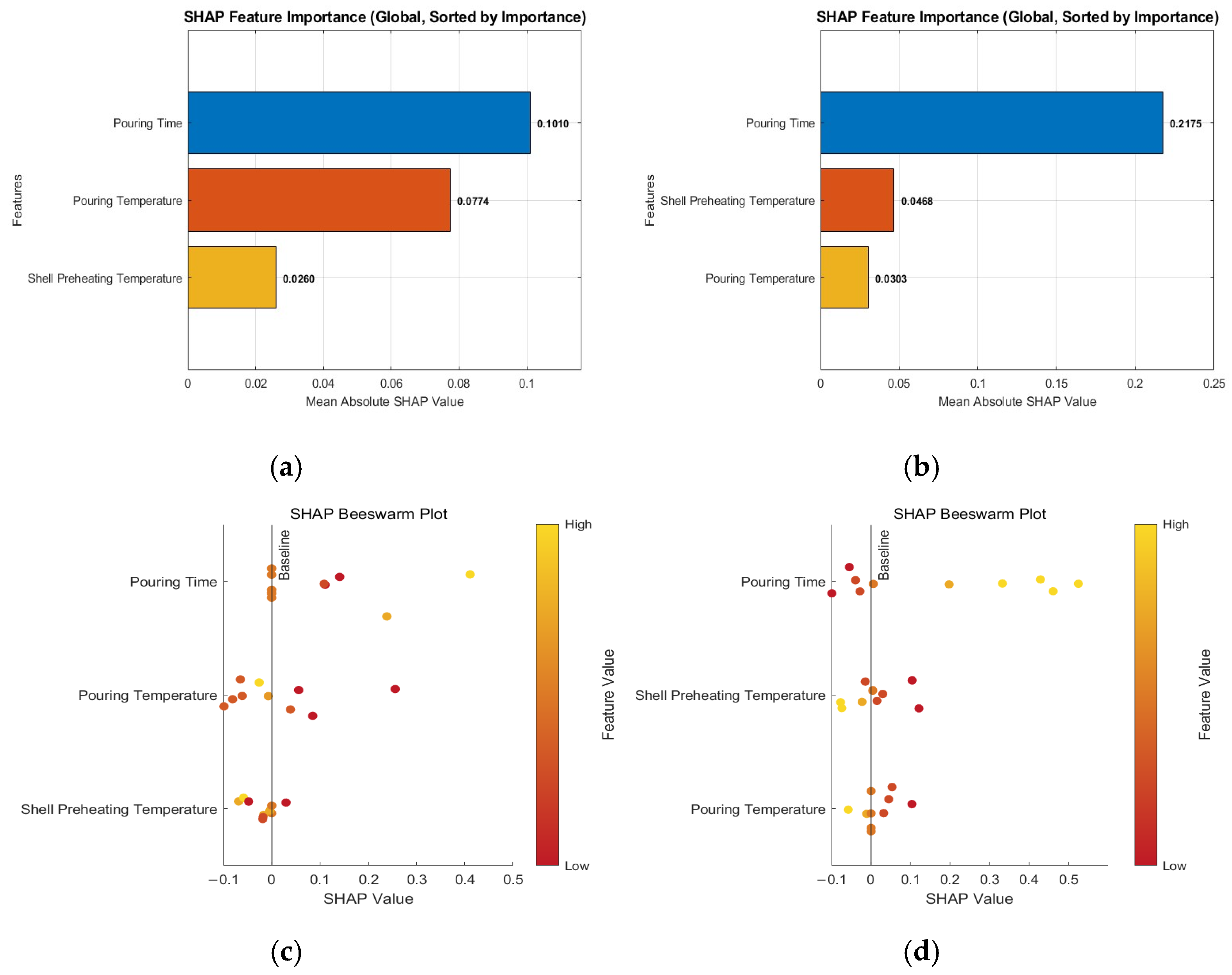
As illustrated in Figure 13, comprehensive SHAP analysis (incorporating bar plots, beeswarm plots, and dependence plots) of the three key process parameters—pouring temperature, pouring time, and shell preheating temperature—in relation to both total defect volume and shrinkage porosity volume yields the following conclusions:

The SHAP global feature importance analysis shows that pouring time is the common core factor affecting both the total defect volume and the shrinkage porosity/void volume, with its SHAP values higher than those of other process parameters, respectively. On this basis, the secondary influencing factors of the two types of defects present obvious differentiation: for the total defect volume, the importance of pouring temperature is significantly higher than that of shell preheating temperature; while for the shrinkage porosity/void volume, the importance of shell preheating temperature surpasses that of pouring temperature. This difference indicates that differentiated parameter regulation logics should be adopted for process optimization targeting different defect types.

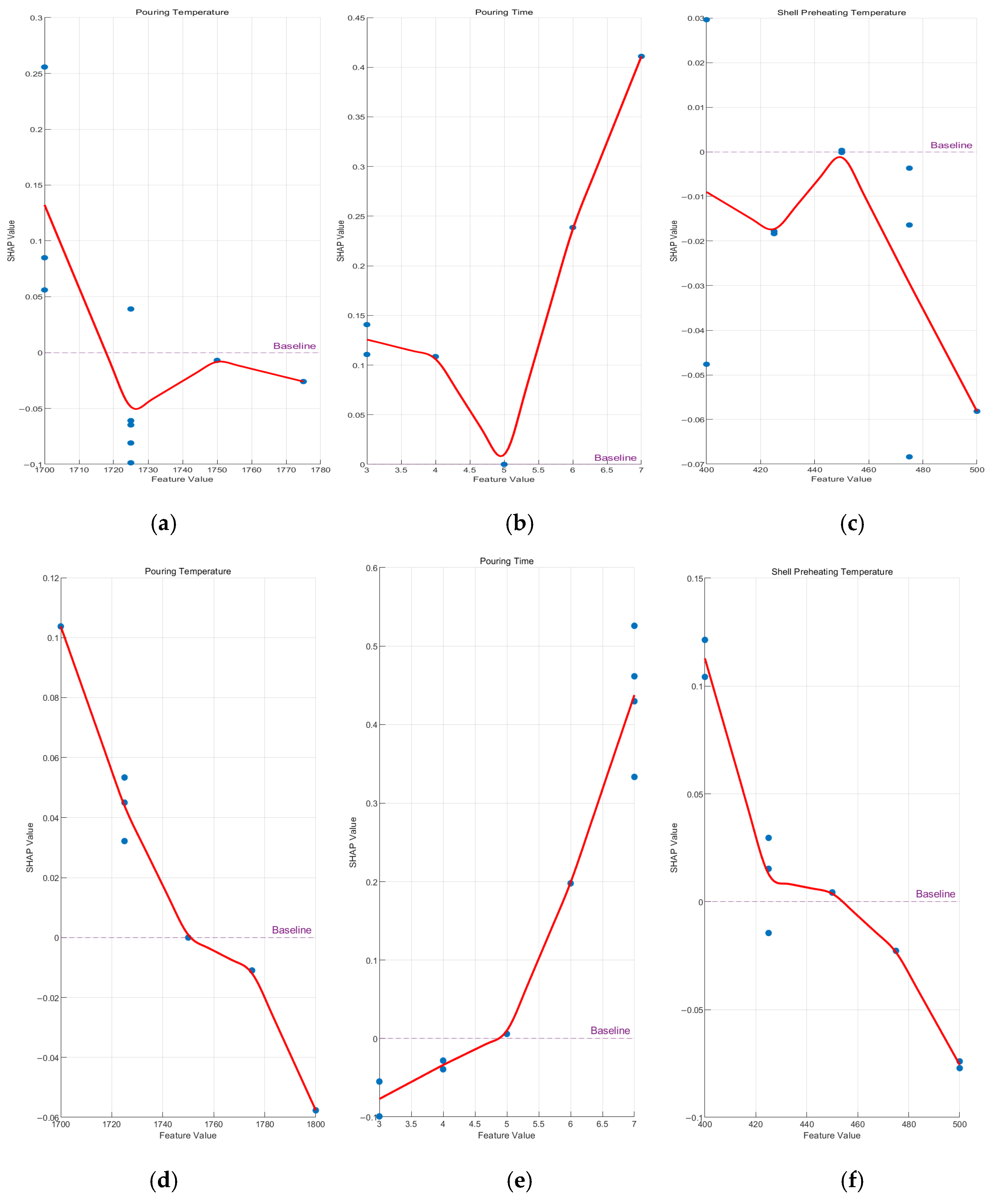
As shown in Figure 14, this set of SHAP feature dependence plots systematically reveals the nonlinear driving mechanisms and differential response characteristics of the three key process parameters (pouring temperature, pouring time, and shell preheating temperature) on total defect volume and shrinkage porosity volume. In these plots, the red line depicts the trend of SHAP values with varying parameter levels, representing the average marginal effect of each parameter on defect formation: values above the purple dashed baseline (SHAP = 0, indicating no impact on defect volume) correspond to an increase in defect volume, while values below correspond to a reduction, with the line slope reflecting the sensitivity of defects to parameter changes. The blue dots denote the SHAP values of individual test samples, where the horizontal position matches the actual parameter value, the vertical position represents the specific contribution of the parameter to the predicted defect volume for that sample, and the dot distribution reflects the dispersion of the parameter’s impact across different process intervals.

For the total defect volume (Figure 14a–c), the driving mechanism exhibits distinct multi-stage nonlinear fluctuation characteristics. Specifically, the effect of pouring temperature (Figure 14a) follows a three-stage rule of defect promotion → inhibition weakening → inhibition enhancement: it promotes defect formation at approximately 1700 °C, the inhibitory effect on defects increases rapidly within 1700–1725 °C, gradually weakens within 1725–1750 °C, and continues to intensify within 1750–1800 °C. Meanwhile, the effect of pouring time (Figure 14b) presents a three-stage nonlinear evolution characteristic of promotion weakening → rapid promotion attenuation → exponential promotion enhancement: the defect-promoting effect weakens with increasing time in the 3–4 s interval; the promoting effect attenuates rapidly in the 4–5 s interval and reaches the weakest negative impact on defect formation at around 5 s; in the 5–7 s interval, it rapidly shifts to a defect-promoting effect with continuously intensifying intensity. Finally, the effect of shell preheating temperature (Figure 14c) shows a three-stage variation rule of inhibition enhancement → inhibition weakening → rapid inhibition enhancement: it exhibits an inhibitory effect on defect formation at approximately 400 °C, the inhibitory effect gradually intensifies within 400–425 °C, its impact on defect formation weakens to the baseline level within 425–450 °C, and it rapidly turns to a strong inhibitory effect with continuously enhancing intensity as the temperature rises within 450–500 °C.

For the shrinkage porosity/void volume (Figure 14d–f), the driving mechanism presents a more significant monotonic or two-stage nonlinear transition characteristic. The effect of pouring temperature (Figure 14d) shows an overall monotonic negative evolution rule: the SHAP value decreases continuously as the temperature rises from 1700 °C to 1800 °C, where the defect-promoting effect weakens gradually in the range of 1700–1750 °C, and it turns to an inhibitory effect after 1750 °C with continuously strengthening intensity. The effect of pouring time (Figure 14e) undergoes a two-stage transition of inhibition attenuation → promotion enhancement: the inhibitory effect on defects weakens gradually with the increase in time in the 3–5 s interval, and it rapidly shifts to a strong defect-promoting effect in the 5–7 s interval with continuously intensifying intensity. The effect of shell preheating temperature (Figure 14f) displays a three-stage evolution of promotion attenuation → negligible effect → inhibition enhancement: it promotes defect formation at approximately 400 °C, the promoting effect weakens gradually with the rise in temperature in the range of 400–425 °C, its impact on defect formation is close to the baseline level within 425–450 °C, and the inhibitory effect increases continuously with the further rise in temperature after 450 °C.

In summary, a comparative analysis of the SHAP dependence plots reveals that the total defect volume and shrinkage porosity/void volume exhibit significantly different response patterns to pouring temperature, pouring time and shell preheating temperature, which uncovers the intrinsic heterogeneity in the formation mechanisms of these two types of defects.

The differences in the above response patterns indicate that differentiated process strategies should be adopted for the precise control of the two types of defects. For the total defect volume, it is necessary to optimize the pouring temperature to the range around 1725 °C or above 1750 °C, regulate the pouring time within the interval of 4–5 s, and maintain the shell preheating temperature above 450 °C; through such multi-stage collaborative regulation, the effective control of the total defect volume can be realized. For shrinkage porosity/void defects, effective inhibition can be achieved by raising the pouring temperature above 1770 °C, controlling the pouring time within 5 s and increasing the shell preheating temperature above 460 °C. The above conclusions provide an important theoretical basis and quantitative support for the precise optimization of casting processes and the targeted control of defects.

5.2. Analysis of Multi-Factor Influence Laws

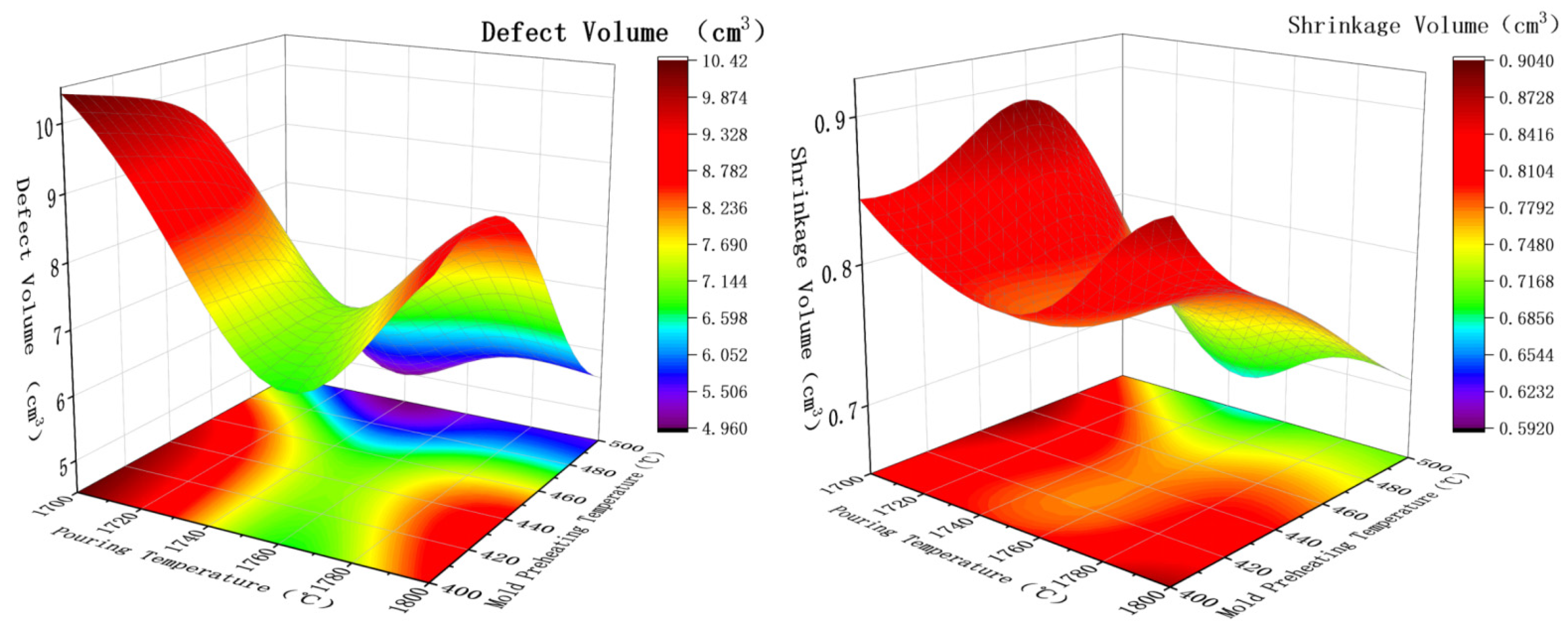
Figure 15, Figure 16 and Figure 17 illustrate the application of the multi-factor analysis, used to evaluate the interactive effects of key process parameters on the total casting defect volume. The parameter settings for the interaction analysis are detailed in

Table 7. Parameters for multi-factor interaction analysis.

Factor	U (°C)	V (s)	W (°C)
1	1750	3~7	400~500
2	1700~1800	5	400~500
3	1700~1800	3~7	450

. Figure 15 shows the coupling effect of pouring temperature and shell preheating temperature on the total defect volume; Figure 16 displays the coupling effect of pouring time and shell preheating temperature; and Figure 17 presents the coupling effect of pouring time and pouring temperature.

Analysis of the results indicates coupling effects among the process parameters—pouring temperature, shell preheating temperature, and pouring time—on both the total defect volume and the shrinkage porosity/void volume. The specific findings are as follows:

When the pouring time is fixed (see Figure 15), the optimal range for the total defect volume corresponds to a pouring temperature of 1740–1760 °C combined with a shell preheating temperature of 480–500 °C. The optimal range for the shrinkage porosity/void volume is similar, falling within a pouring temperature of 1750–1800 °C and a shell preheating temperature of 480–500 °C.

When the pouring temperature is held constant (see Figure 16), the optimal range for the total defect volume is a pouring time of 4.0–6.0 s and a shell preheating temperature of 480–500 °C. The optimal range for the shrinkage porosity/void volume, under this condition, is a pouring time of 3.0–5.5 s and a shell preheating temperature of 460–500 °C.

When the shell preheating temperature is kept constant (see Figure 17), the optimal range for the total defect volume is a pouring time of 3.0–4.0 s and a pouring temperature of 1700–1730 °C. The optimal range for the shrinkage porosity/void volume, under this condition, is a pouring time of 3.0–4.0 s and a pouring temperature of 1780–1800 °C.

In summary, Analysis of Multi-Factor Influence Laws reveals that the sensitivity of pump body defects to process parameters follows this descending order: pouring time, pouring temperature, and shell preheating temperature. Furthermore, contour analysis demonstrates that the coupling effect between pouring temperature and pouring time has the most significant impact on both total defect volume and shrinkage porosity, while the interaction between pouring temperature and shell preheating temperature shows the least coupling influence.

6. Multi-Objective Parameter Optimization

6.1. Fundamental Principles of the NSGA-II Algorithm

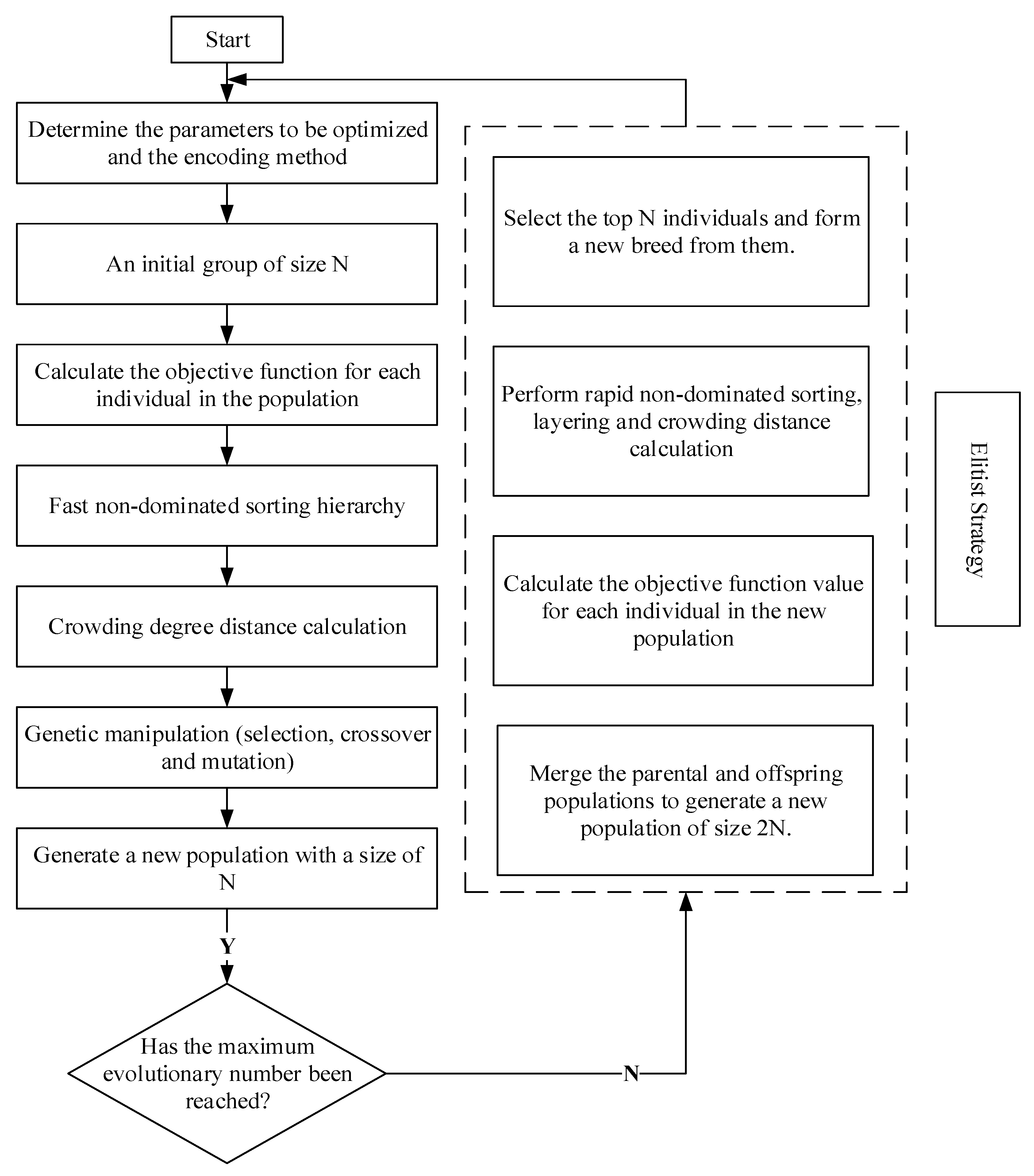
NSGA-II is a multi-objective optimization algorithm based on genetic algorithms. It stratifies the population through non-dominated sorting, maintains solution diversity using crowding distance, and incorporates an elitist strategy by combining parent and offspring populations before selection, thereby ensuring both convergence and diversity during the optimization process [31].

The algorithm workflow is illustrated in Figure 18 and proceeds as follows: First, the problem solutions are encoded as chromosomes (e.g., binary strings). After randomly generating an initial population, the fitness of each individual is evaluated. It is important to note that in NSGA-II, the concept of fitness is primarily embodied by the non-dominated rank and the crowding distance during the selection stage. The algorithm employs fast non-dominated sorting to stratify individuals into different frontier levels (ranks) based on Pareto domination relationships. This is combined with the crowding distance (a measure related to the perimeter of the hypercube formed by an individual’s nearest neighbors) to maintain population diversity. The selection operation prioritizes individuals with better (lower) ranks and those located in sparser regions (larger crowding distance). Crossover is applied to enhance global search capability, while mutation improves local search efficiency. The elitist strategy, which merges the parent and offspring populations before selecting the next generation, helps prevent the loss of high-quality individuals. The population is iteratively updated until specific convergence criteria are met (e.g., finding the Pareto-optimal set, reaching the maximum number of generations, or achieving stabilization in the population’s fitness distribution). Through this cooperative multi-objective optimization mechanism, the algorithm efficiently identifies a well-distributed approximation of the Pareto-optimal front within the solution space.

Input: Decision variables (pouring temperature: 1700–1800 °C, pouring time: 3–7 s, shell preheating temperature: 400–500 °C); population size: 100; number of iterations: 100

Output: Pareto-optimal solution set.

Step 1: Initialize the population $P_0$, and calculate the objective function values (total defect volume, shrinkage cavity volume) for each individual.

Step2: Perform non-dominated sorting on $P_0$, calculate the crowding distance, and select the top 100 individuals as the parent population $P_t$.

Step 3: For t = 1 to 100:

a. Crossover: Generate the offspring population $Q_t$ (size: 100) using Simulated Binary Crossover (SBX).

b. Mutation: Perform polynomial mutation (mutation step size: 0.1).

c. Merge Pt and $Q_t$ to obtain the population $R_t$ (size: 200).

d. Perform non-dominated sorting on $R_t$ to divide it into Front 1, Front 2,...

e. Calculate the crowding distance of each Front, and select 100 individuals as the next-generation population $P_{t+1}$ based on “Front priority + crowding distance”.

f. If the change rate of objective values of Front 1 is <0.1% for 10 consecutive generations, stop the iteration in advance.

Step 4: Output the final Front 1 as the Pareto-optimal solution set.

6.2. Optimization Results of NSGA-II

Based on the optimized ranges of key process parameters, the NSGA-II algorithm is employed to screen for relatively optimal parameters. NSGA-II (Non-dominated Sorting Genetic Algorithm II) is a significant improvement of genetic algorithms in the field of multi-objective optimization. It is designed to solve optimization problems with multiple conflicting objectives and to generate a Pareto-optimal solution set.

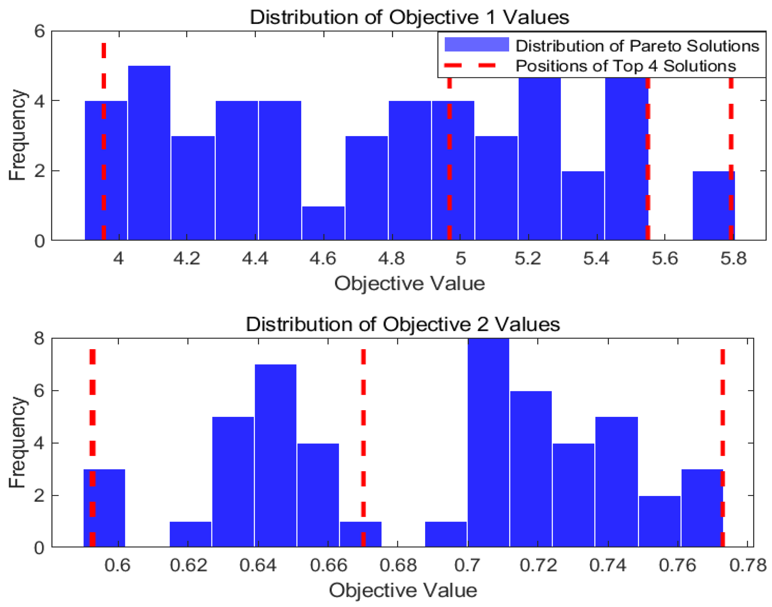
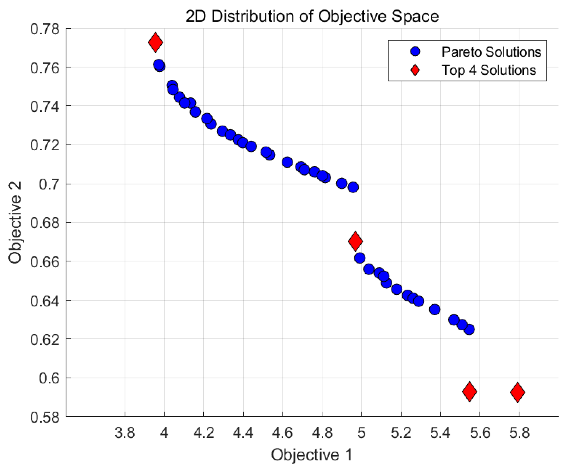
Figure 19 displays the distribution histograms of the Pareto-optimal solution set generated by the NSGA-II algorithm for Objective 1 and Objective 2 in the context of titanium alloy investment casting, with the red dashed lines marking the single-objective optimal positions for each objective. The corresponding Pareto-optimal solution set is visualized in Figure 20. Furthermore, simulation verification of the optimal solution set was conducted using ProCAST, and a comparative analysis of the total defect volume and shrinkage porosity volume is summarized in

Table 8. Pareto-optimal solution set.

	Pouring Temperature (°C)	Pouring Time (s)	Shell Preheating Temperature (°C)	Pred. Total Vol. (cm3)	Pred. Shrinkage Vol. (cm3)	Sim. Total Vol. (cm3)	Sim. Shrinkage Vol. (cm3)
1	1800	4	475	6.156584325	0.624084359	6.125182	0.62823155
2	1725	5	500	5.289102648	0.706907094	5.741780	0.632726
3	1750	4	450	7.587146024	0.691785429	7.507708	0.662608
4	1700	4	450	6.381000493	0.820719872	6.40854	0.769607

.

6.3. Error Analysis and Optimization Results

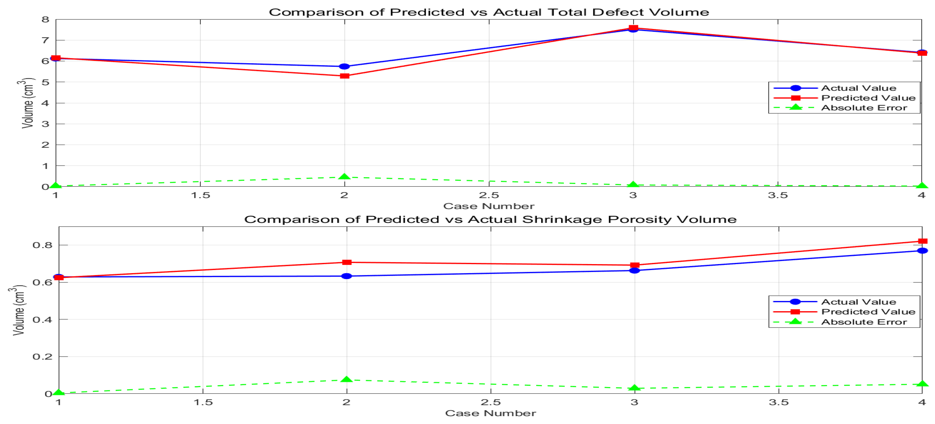
The prediction errors for the defects are shown in Figure 21 The error for the total defect volume remains within a relatively small range overall (with a maximum error of less than 1 cm³), and the error curve exhibits a smooth trend. Meanwhile, the error for the shrinkage porosity/void volume consistently remains at an extremely low level (less than 0.1 cm³), with minimal fluctuation across different test cases. This indicates that the model achieves excellent predictive performance, meeting the expected performance targets.

Among various factors leading to casting scrap in industrial production, including shrinkage porosity/shrinkage cavity, surface scars, and cracking during the straightening process, shrinkage porosity and shrinkage cavity are the core causes of the persistently high scrap rate of castings. In addition, the remediation of shrinkage cavity defects requires complex post-treatment procedures, and areas with severe shrinkage cavities generally present higher stress concentration. In combination with these practical production requirements, the parameter combination with a pouring temperature of 1800 °C, a pouring time of 4 s, and a shell preheating temperature of 475 °C is selected as the superior process parameter set.

From the perspective of casting physics, the core mechanism and superiority of this optimized parameter combination lie in the establishment of thermodynamic and kinetic conditions conducive to sequential solidification and effective feeding through the collaborative regulation of the temperature field and mold filling process. The relatively high pouring temperature significantly improves the superheat and fluidity of the molten metal, which not only ensures the complete filling of complex cavities to reduce mold filling defects such as cold shuts, but also prolongs the overall solidification time of the molten metal to reserve a sufficient feeding window. In conjunction with the extremely short pouring time, the molten metal completes cavity filling almost synchronously in a high-temperature and rapid state, obtaining a uniform initial temperature field to avoid premature solidification and blockage of the feeding channel caused by sequential filling. Meanwhile, the high shell preheating temperature greatly reduces the temperature difference between the casting and the mold, and smoothens the overall solidification process. This synergistic combination of high-temperature rapid pouring and high mold preheating ultimately forms a sequential solidification temperature gradient from the position far away from the gate to the gate direction, keeping the feeding channel open for a long time during the critical stage of solidification shrinkage, thus achieving sufficient feeding in the solidification shrinkage stage, and simultaneously and drastically reducing the most harmful micro shrinkage porosity and centralized shrinkage cavities from the physical root.

In terms of manufacturability, this parameter combination greatly improves the mold filling adaptability of complex cavities and the controllability of solidification quality, and significantly reduces the probability of casting scrap and rework caused by mold filling defects and internal defects. Meanwhile, the uniform temperature field and smooth solidification process reduce the internal stress concentration of the casting, alleviate the stress concentration problem in the shrinkage cavity area, further lower the cracking risk in the subsequent straightening process, and improve the process compatibility and finished product stability of the full production process, while only putting forward higher adaptation requirements for the filling precision and stability of the pouring equipment, as well as the high-temperature thermal stability and refractory performance of the shell.

In terms of thermal risk, this scheme greatly mitigates the thermal stress and hot cracking risk caused by the rapid cooling of the casting surface, as well as the in-service and straightening cracking risks caused by stress concentration at defect locations by reducing the interfacial temperature difference between the casting and the mold, and constructing a uniform initial temperature field and a directional sequential solidification mode, with the core thermal hazards effectively controlled.

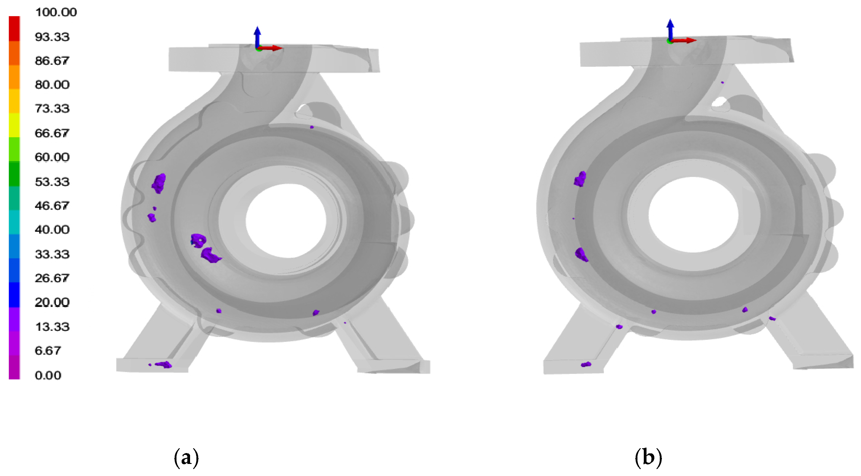
Simulation verification was carried out based on this ideal optimized parameter combination, and the comparison results are shown in Figure 22a,b display the defect distributions corresponding to the original process scheme (1725 °C, 7 s, 400 °C) and the optimized scheme, respectively. The comparison reveals that the total defect volume is significantly reduced. The predicted total defect volume decreases from 10.027715 cm³ to 6.125 cm³ (a reduction of approximately 38.92%), and the shrinkage porosity/shrinkage cavity volume drops from 1.298505 cm³ to 0.6282 cm³ (a reduction of approximately 51.62%). This indicates that the casting defects have been further optimized.

7. Conclusions

In this study, an L₂₅(5³) orthogonal simulation experiment combined with random sampling was first adopted to construct a complete dataset covering the full domain of key process parameters for ZTA2 titanium alloy investment casting. Aiming at the local optimum and poor generalization problems of the standard BP neural network in casting defect prediction, a BP neural network optimized by the PSO algorithm was developed, and a corresponding high-precision defect prediction model was established for quantitative analysis and accurate prediction of casting defects. Subsequently, the NSGA-II algorithm was employed to search for relatively optimal solutions, and the relatively optimal process parameter combination for investment casting was obtained. The main conclusions are as follows:

(1) Verified by 5-fold cross-validation, the optimized PSO-BP (Bayesian regularization) neural network prediction model exhibits excellent prediction precision and generalization ability. Compared with the traditional BP neural network, the performance of the optimized model is significantly improved, with the specific results as follows:

For the prediction of total defect volume, the coefficient of determination (R²) of the test set is increased by 20.82%, and the root mean square error (RMSE) is reduced by 33.34%;

For the prediction of shrinkage porosity/void volume, the test set R² is increased by 7.93%, and the RMSE is reduced by 22.71%.

This effectively solves the problems of the traditional BP network, such as being prone to falling into local optima and weak generalization ability.

(2) Through orthogonal experiment analysis and SHAP-based parameter sensitivity analysis, it is found that pouring time is the most important factor affecting defect volume, and its influence degree is significantly higher than that of pouring temperature and shell preheating temperature. Further two-factor interaction analysis shows that the combination of pouring temperature and pouring time exhibits the strongest coupling effect on both total defect volume and shrinkage porosity/void volume, while the interaction between pouring temperature and shell preheating temperature has the weakest coupling influence.

(3) Combined with the NSGA-II algorithm, a set of superior process parameter combinations was determined. Considering the actual production conditions, the parameter combination with a pouring temperature of 1800 °C, a pouring time of 4 s, and a shell preheating temperature of 475 °C was selected as the superior solution. Compared with the pre-optimization results, this superior solution reduces the total defect volume by 38.92% and the shrinkage porosity/void volume by 51.62%, achieving a significant defect control effect.

References

1. Yuan, X.G.; Wang, Y.X.; Zheng, B.W. Research progress and prospects of cast non-ferrous alloys: Review of the non-ferrous alloy forum at the 75th World Foundry Congress. Foundry 2025, 74, 1013–1028. [Google Scholar]
2. Luo, S.H. Microstructure and Properties Evolution of ZTA2 Commercial Pure Titanium During Power Spinning and Heat Treatment; Taiyuan University of Technology: Taiyuan, China, 2024. [Google Scholar]
3. Lyu, W.J.; Zhang, D.; Han, Y.F.; Le, J.W.; Hou, Z.J.; Wang, P.L. Review on Preparation, Processing and Application of Heat-Resistant Titanium Matrix Composites. Aeronaut. Manuf. Technol. 2023, 66, 38–47+71. [Google Scholar] [CrossRef]
4. Zhang, P.F.; Zhang, L.J.; Zhou, Y.; Sun, F.; Wang, J.; Li, J.S. Advances in Application of Titanium Alloy Precision Casting Technology in the Aerospace Field. Aeronaut. Manuf. Technol. 2025, 68, 22–36. [Google Scholar] [CrossRef]
5. Ran, X.; Chen, Y.S.; Gao, X.H.; Long, X.Q.; Fu, Z.P.; He, L.J.; Li, P.J. Casting Simulation and Analysis of Shrinkage Porosity Defects for Large Titanium Alloy Casings by Centrifugal Precision Casting. Foundry 2025, 74, 344–349. [Google Scholar]
6. Yu, W.; Qie, X.; Zhao, W.; Nan, H.; Wu, G. Effect of structural features on microstructure and properties homogeneity based on quantification and statistical analysis for large-scaled complex titanium alloy castings. Int. J. Met. 2024, 18, 1535–1546. [Google Scholar] [CrossRef]
7. Sun, H.; Wang, M.M.; Zhang, X.Y.; Cai, Y.Q.; Sun, L.R.; Li, D.D.; Zhou, C.Y.; Dong, X.L. Research Progress on Casting Process and Numerical Simulation of Large Castings. Ordnance Mater. Sci. Eng. 2026, 49, 200–214. [Google Scholar] [CrossRef]
8. Qie, X.W.; Li, W.; Yin, Y.J.; Xu, Q.; Nan, H.; Zhou, J.X. Effect of Centrifugal Casting Process Parameters on Shrinkage Porosity Defects and Microstructure of Titanium Alloy Thin-Walled Support Plates. Spec. Cast. Nonferrous Alloys 2024, 1–7. [Google Scholar]
9. Liu, T.J. Numerical Simulation of Centrifugal Casting for Titanium Alloy Impeller. Master’s Thesis, Harbin Institute of Technology, Harbin, China, 2014. [Google Scholar]
10. Pan, D.; Xu, Q.Y.; Liu, B.C. Three-dimensional microstructure simulation of Ni-based superalloy investment castings. Sci. China Phys. Mech. Astron. 2011, 54, 851–855. [Google Scholar] [CrossRef]
11. Sata, A.; Ravi, B. Comparison of some neural network and multivariate regression for predicting mechanical properties of investment casting. J. Mater. Eng. Perform. 2014, 23, 2953–2964. [Google Scholar] [CrossRef]
12. Manjunath Patel, G.C.; Shettigar, A.K.; Krishna, P.; Parappagoudar, M.B. Back propagation genetic and recurrent neural network applications in modelling and analysis of squeeze casting process. Appl. Soft Comput. 2017, 59, 418–437. [Google Scholar] [CrossRef]
13. Dong, Y.; Guo, X.; Ye, Q.; Yan, W. Shrinkage during solidification of complex structure castings based on convolutional neural network deformation prediction research. Int. J. Adv. Manuf. Technol. 2022, 118, 4073–4084. [Google Scholar] [CrossRef]
14. Yu, W.Y.; He, F.S.; Yao, Y.; Huang, Y.; Xiang, H.L.; Huang, J.L. Optimization of Casting Process for Engine Stainless Steel Accessories Based on Combination of PSO-BP and GA. Mech. Sci. Technol. Aerosp. Eng. 2025, 44, 1966–1973. [Google Scholar] [CrossRef]
15. Yu, P.; Ji, X.; Sun, T.; Zhou, W.; Li, W.; Xu, Q.; Qie, X.; Yin, Y.; Shen, X.; Zhou, J. Data-Physics Fusion-Driven Defect Predictions for Titanium Alloy Casing Using Neural Network. Materials 2024, 17, 2226. [Google Scholar] [CrossRef]
16. Shao, Y.J.Q.; Qian, C.H. Application and prospect of artificial neural network in casting process. Met. Work. (Hot Work.) 2025, 6, 13–21. [Google Scholar]
17. Liu, X.; Dong, A.; Wang, D.; Lu, Y.; Zhu, G. Numerical simulation and optimization of casting process for complex pump. IOP Conf. Ser. Mater. Sci. Eng. 2017, 231, 012134. [Google Scholar] [CrossRef]
18. Peng, W.W.; Zheng, J.N.; Yan, T.; Yu, S.Q. Research on Investment Casting Process and Equipment. In Proceedings of the Symposium on Technical Paper Exchange of Electromechanical Equipment Technology and Cultivation and Development of Technical Talents; China Electromechanical Equipment Maintenance and Transformation Technology Association: Beijing, China, 2025. [Google Scholar] [CrossRef]
19. Sun, F.S.; Pang, F.; Liu, M.Q. Construction of column-orthogonal designs for computer experiments. Sci. China Math. 2011, 54, 2683–2692. [Google Scholar] [CrossRef]
20. Panzhong, L.; Ning, L. Low pressure casting technology and forming process analysis of metal mold based on ProCAST FEA procedure. Mech. Adv. Mater. Struct. 2022, 29, 1308–1315. [Google Scholar] [CrossRef]
21. Van den Heuvel, E.; Zhan, Z. Myths about linear and monotonic associations: Pearson’s r, Spearman’s ρ, and Kendall’s τ. Am. Stat. 2022, 76, 44–52. [Google Scholar] [CrossRef]
22. Feng, Q.; Li, Q.; Quan, W.; Pei, X. A survey of multi-objective particle swarm optimization algorithm. Chin. J. Eng. 2021, 43, 745–753. [Google Scholar]
23. Hu, Y.M. Research on Scheduling and Sequencing of Mixed-Model Assembly Line with Multi-Variety and Small-Batch Under JIT Production Mode. Master’s Thesis, Changchun University of Technology, Changchun, China, 2015. [Google Scholar]
24. Sheng, W.B. Research on Breakout Prediction System Based on BP Neural Network Optimized by Ant Colony Algorithm. Master’s Thesis, Yancheng Institute of Technology, Yancheng, China, 2023. [Google Scholar]
25. Deng, J.; Liu, G.; Wang, L.; Liu, G.; Wu, X. Intelligent optimization design of squeeze casting process parameters based on neural network and improved sparrow search algorithm. J. Ind. Inf. Integr. 2024, 39, 100600. [Google Scholar] [CrossRef]
26. Xu, S.; Xu, X.; Jia, W.; Liu, W.; Li, J.; Li, D. Microstructure-property map** modeling for AZ31 alloy rolling deformation using improved PSO-BP neural network. J. Mater. Res. Technol. 2023, 25, 2127–2139. [Google Scholar] [CrossRef]
27. Ismail, A.; Jeng, D.-S.; Zhang, L. An optimized product unit neural network with a novel PSO-BP hybrid training algorithm: Applications to load-deformation analysis of axially loaded piles. Eng. Appl. Artif. Intell. 2013, 26, 2305–2314. [Google Scholar] [CrossRef]
28. Li, X.H.; Li, Z.C. Research progress and key technologies of artificial neural network in predicting dynamic recrystallization. Chin. J. Nonferrous Met. 2024, 34, 2547–2558. [Google Scholar]
29. Clerc, M.; Kennedy, J. The particle swarm–explosion, stability, and convergence in a multidimensional complex space. IEEE Trans. Evol. Comput. 2002, 6, 58–73. [Google Scholar] [CrossRef]
30. Wang, D.; Li, M. Performance Analysis and Parameter Selection of Particle Swarm Optimization Algorithm. Acta Autom. Sin. 2016, 42, 1552–1561. [Google Scholar]
31. Deb, K.; Pratap, A.; Agarwal, S.; Meyarivan, T. A fast and elitist multiobjective genetic algorithm: NSGA-II. IEEE Trans. Evol. Comput. 2002, 6, 182–197. [Google Scholar] [CrossRef]
Figure 1. Three-dimensional model of the pump body: 1. Outlet flange 2. Inlet flange 3. Shell cover flange 4. Flow passage 5. Base.
Coatings 16 00589 g001
Figure 2. Simulation setup procedure.
Coatings 16 00589 g002
Figure 3. Simulated shrinkage evolution results of titanium alloy pump body casting in two solidification processes. (a) Pouring temperature 1725 °C; (b) Pouring temperature 1800 °C.
Coatings 16 00589 g003
Figure 4. Effects of pouring temperature, pouring time, and shell preheating temperature on the total defect volume and the shrinkage porosity/void volume. In the three-dimensional surface plots, the total defect volume is represented in blue, and the shrinkage porosity/void volume is represented in red, with the legend for the total defect volume (blue) placed in the upper left corner and that for the shrinkage porosity/void volume (red) placed in the upper right corner, differentiated by the boundary of the 4% critical porosity rate [20].
Coatings 16 00589 g004
Figure 5. Flowchart of the Particle Swarm Optimization (PSO) algorithm.
Coatings 16 00589 g005
Figure 6. Structure of the BP neural network.
Coatings 16 00589 g006
Figure 7. Function graphs. (a) Hyperbolic tangent function (tansig); (b) Linear function (purelin).
Coatings 16 00589 g007
Figure 8. (a) Single-Factor Sensitivity Analysis Curve of Hidden Neuron Number. (b) Single-Factor Sensitivity Analysis Curve of BP Learning Rate. (c) Single-Factor Sensitivity Analysis Curve of PSO Population Size. (d) Single-Factor Sensitivity Analysis Curve of PSO Iteration Number. (e) Single-Factor Sensitivity Analysis Curve of PSO Learning Factor Combinations. (f) Comparative Analysis of Sensitivity Coefficients for 5 Core Parameters.
Coatings 16 00589 g008aCoatings 16 00589 g008b
Figure 9. (a) 5-Fold Cross Validation-Based Prediction Performance Comparison Chart for Total Defect Volume (RMSE and R2) (b) 5-Fold Cross Validation-Based Prediction Performance Comparison Chart for Shrinkage Porosity/Void Volume (RMSE and R2).
Coatings 16 00589 g009
Figure 10. (a) Total Defect Volume Prediction: PSO Iteration Fitness Error Variation Curve (b) Shrinkage Porosity/Void Volume Prediction: PSO Iteration Fitness Error Variation Curve.
Coatings 16 00589 g010
Figure 11. Comparison of Fitting Effect and Predictive Performance of the Total Defect Volume Prediction Model (a) Comparison Curve of Predicted and Actual Values in the Training Set (b) Comparison Curve of Predicted and Actual Values in the Test Set (c) Scatter Fitting Plot of Predicted vs. Actual Values in the Training Set (d) Scatter Fitting Plot of Predicted vs. Actual Values in the Test Set.
Coatings 16 00589 g011aCoatings 16 00589 g011b
Figure 12. Comparison of Fitting Effect and Predictive Performance of the Shrinkage Porosity/Void Volume Prediction Model (a) Comparison Curve of Predicted and Actual Values in the Training Set (b) Comparison Curve of Predicted and Actual Values in the Test Set (c) Scatter Fitting Plot of Predicted vs. Actual Values in the Training Set (d) Scatter Fitting Plot of Predicted vs. Actual Values in the Test Set.
Coatings 16 00589 g012
Figure 13. SHAP Analysis of Casting Defect Prediction Models (a) SHAP Feature Importance (Total Defect Volume) (b) SHAP Feature Importance (Shrinkage Porosity/Void Volume) (c) SHAP Beeswarm Plot (Total Defect Volume) (d) SHAP Beeswarm Plot (Shrinkage Porosity/Void Volume).
Coatings 16 00589 g013
Figure 14. SHAP Single Feature Dependence Plots, (ac) represent the total defect volume and (df) represent the shrinkage porosity/void volume. (a,d) stand for pouring temperature, (b,e) for pouring time, and (c,f) for shell preheating temperature.
Coatings 16 00589 g014
Figure 15. Relationship between pouring temperature and shell preheating temperature.
Coatings 16 00589 g015
Figure 16. Relationship between pouring time and shell preheating temperature.
Coatings 16 00589 g016
Figure 17. Relationship between pouring temperature and pouring time.
Coatings 16 00589 g017
Figure 18. NSGA-II algorithm flow.
Coatings 16 00589 g018
Figure 19. Histogram of the Optimal Solution Set Distribution.
Coatings 16 00589 g019
Figure 20. Pareto-optimal solution set.
Coatings 16 00589 g020
Figure 21. Predicted Defect Error Value.
Coatings 16 00589 g021
Figure 22. Comparison of defects before and after optimization. (a) Defect distribution corresponding to the original parameter scheme. (b) Defect distribution corresponding to the optimized parameter scheme.
Coatings 16 00589 g022