Deep Spatiotemporal Condition Monitoring and Subsystem Fault Classification for Selective Laser Melting Equipment

Abstract

The integration of Selective Laser Melting (SLM) into high-end manufacturing necessitates robust machine-condition monitoring and subsystem fault classification to navigate the intricate coupling and dynamic transients inherent in these systems. Current diagnostic frameworks often struggle to decouple high-dimensional state variables or track their underlying temporal evolution. To overcome these bottlenecks, this paper develops a spatiotemporal deep learning architecture by coupling Convolutional Neural Networks (CNNs) with Long Short-Term Memory (LSTM) units. This hybrid approach leverages CNNs to distill multi-dimensional spatial features from subsystem sensor arrays, while LSTMs interpret the sequential dependencies critical for identifying systemic drifts. The proposed framework was validated using an extensive industrial dataset comprising over 310,000 temporal samples across seven critical SLM subsystems, including optical, cooling, and energy units. We systematically investigated three data-handling strategies—feature weighting, balancing, and distribution-based synthesis—to optimize the model’s sensitivity to rare-event anomalies. Benchmarking across six architectural variants reveals that a specific CNN × 3 + LSTM × 1 configuration yields superior diagnostic fidelity, achieving a classification accuracy of 98.81%. Visualization of the feature space confirms high inter-class separability, demonstrating the model’s ability to isolate faults within complex manufacturing cycles. This research offers a scalable paradigm for the intelligent monitoring of SLM equipment and provides a technical benchmark for equipment health management and predictive maintenance in advanced additive manufacturing.

1. Introduction

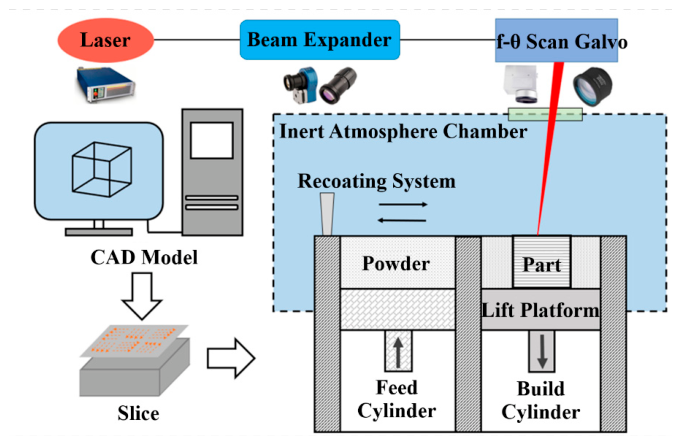
Selective Laser Melting has emerged as a cornerstone of metal additive manufacturing (AM), enabling the stochastic-to-deterministic synthesis of high-precision, geometrically complex components through layer-by-layer laser-powder interaction (Figure 1). The inherent advantages of SLM—unprecedented design freedom, high material utilization, and superior mechanical properties—have catalyzed its strategic adoption across the aerospace, biomedical, and precision engineering sectors [1].

However, the industrial maturation of SLM is hindered by the extreme sensitivity of the process to multi-physics transients. An SLM machine functions as a tightly coupled system of systems, integrating laser optics, thermo-fluid dynamics within the build chamber, and high-precision motion control. Such high-dimensional complexity renders the process susceptible to a spectrum of stochastic anomalies, ranging from subtle laser power fluctuations to critical powder recoating inconsistencies or shielding gas disturbances [2]. These anomalies, if undetected, propagate through the build cycle, compromising metallurgical integrity or manifesting as catastrophic system failures.

In addressing these challenges, it is crucial to delineate the scope of monitoring. While in situ process-defect detection relies on high-frequency (e.g., kHz level) sensing to capture micro-scale melt-pool dynamics, machine-condition monitoring utilizes low-frequency telemetry (e.g., 1 Hz) to evaluate the macro-environmental and mechanical stability of the equipment. This study explicitly focuses on the latter. By classifying subsystem faults before they precipitate macroscopic build defects, this framework serves as a critical prerequisite for maintaining the stable operational environment required for high-quality SLM.

Traditional monitoring paradigms—predominantly relying on heuristic thresholds or expert-defined rule sets—frequently fail to generalize across the non-stationary dynamics of SLM processes, leading to excessive false alarms or missed latent fault detections [3]. While the proliferation of Industrial Internet of Things (IIoT) sensors has generated a deluge of multivariate time-series data, translating these high-throughput streams into actionable diagnostic intelligence remains a non-trivial challenge. Specifically, three bottlenecks persist:

• Systemic Coupling & Dimensionality: The interdependencies between heterogeneous subsystems (e.g., optical vs. gas circulation) create a high-dimensional feature space where anomalous signatures are often masked by cross-channel noise [4].
• Temporal Non-stationarity: SLM faults are rarely instantaneous; they often manifest as gradual drifts or context-dependent deviations that necessitate the modeling of long-range temporal dependencies [5].
• Class Imbalance & Label Scarcity: In production environments, the overwhelming dominance of “steady-state” data renders traditional supervised classifiers prone to overfitting, failing to capture the rare but critical “tail” of the anomaly distribution [6].

To bridge these gaps, this study develops a deep spatiotemporal anomaly detection framework specifically architected for the multi-system constraints of SLM equipment. Rather than treating sensor data as disjointed signals, our approach employs a hybrid CNN-LSTM topology: CNNs serve as spatial encoders to distill inter-subsystem correlations, while LSTM units function as temporal decoders to track the evolution of the state space.

The core contributions of this work are threefold:

• Domain-Guided Data Synthesis: We propose three distinct data construction strategies—feature weighting, balancing, and comprehensive distribution—to systematically address the data scarcity in multi-class anomaly detection across seven SLM subsystems.
• Spatiotemporal Feature Fusion: A dual-path architecture is introduced to resolve the “horizontal” spatial coupling and “vertical” temporal dependencies simultaneously, enhancing the granularity of fault isolation in complex industrial cycles.
• Empirical Benchmarking: Through extensive validation on real-world industrial datasets, we quantify the trade-offs between model depth and diagnostic fidelity, providing a technical roadmap for the deployment of intelligent predictive maintenance in advanced manufacturing.

2. Related Work

2.1. Anomaly Detection in Additive Manufacturing (AM)

The proliferation of AM in mission-critical sectors has necessitated real-time diagnostic frameworks capable of navigating the stochastic nature of laser-powder interactions and thermo-fluid dynamics. Early efforts in process monitoring primarily focused on identifying discrete failure modes through localized sensing. For instance, acoustic emission (AE) and vibration signatures have been extensively utilized to detect nozzle clogging in Fused Filament Fabrication (FFF) and resin-print inconsistencies in Digital Light Processing (DLP) [7,8]. Comprehensive reviews by Sampedro et al. [9] and Chen et al. [10] emphasize that while conventional machine learning—such as SVMs and clustering—can achieve high accuracy (up to 97%) in polymer-based AM, these models often falter when faced with the high-dimensional, cross-system coupling inherent in metal-based SLM.

Recent transitions toward wire-fed and laser-based metal AM have introduced multi-sensor integration (e.g., optical, thermal, and atmospheric sensors) to monitor temperature and gas flow disturbances [11,12]. However, a significant portion of the current literature remains siloed within single-sensor paradigms. These approaches frequently overlook the inter-system correlations, failing to account for how an anomaly in the cooling subsystem might latently propagate into the optical or energy modules.

2.2. Deep Learning Paradigms in Industrial Diagnostics

To bypass the limitations of manual feature engineering, deep learning (DL) has been adopted to autonomously extract hierarchical representations from raw industrial telemetry [13]. CNNs have proven effective in distilling spatial patterns from vibration and network signals [14], while Recurrent Neural Networks (RNNs), specifically LSTM units, have set benchmarks in modeling the temporal evolution of sensor drifts and energy fluctuations [15,16].

Despite the high-fidelity representation offered by DL, existing frameworks in AM predominantly address data scarcity through unsupervised generative models, such as GANs and autoencoders (AEs) [17,18]. While these methods mitigate class imbalance, they often operate as “black boxes” with limited interpretability. More critically, most current models are optimized for either spatial feature extraction or temporal sequencing in isolation, creating a systemic gap in capturing the simultaneous spatiotemporal transients that characterize SLM failures.

2.3. Spatiotemporal Modeling in Complex Systems

The operational state of an SLM machine is defined by a dense spatiotemporal coupling: spatial interactions occur across heterogeneous subsystems, while anomalies evolve and propagate over discrete temporal scales. Spatiotemporal architectures, which fuse CNN-based spatial encoders with recurrent temporal decoders, have recently shown promise in adjacent fields such as water quality monitoring [19], photovoltaic diagnostics [20], and chemical process control [21]. For example, the integration of attention mechanisms with Bi-LSTM units has significantly enhanced noise suppression and long-term dependency modeling in high-dimensional datasets [21,22].

Recently, the paradigm of SLM diagnostics has begun to shift from analyzing isolated, single-modal sensors (e.g., high-speed cameras or acoustic emission) toward multi-system sensor fusion [23]. While localized sensors excel at detecting micro-scale melt-pool anomalies [24,25], they often fail to capture macro-environmental drifts—such as shielding gas turbulence or holistic thermal accumulation—that ultimately precipitate these local defects. Consequently, capturing the highly coupled interactions among the mechanical, optical, and fluidic subsystems necessitates advanced spatiotemporal modeling, which serves as the primary motivation for the CNN-LSTM architecture proposed in this study.

However, the application of such integrated spatiotemporal frameworks to SLM remains remarkably sparse. Current SLM monitoring research is largely confined to 2D melt-pool imaging or single-subsystem tracking, lacking a holistic architecture that reconciles the “horizontal” correlation between multiple subsystems with the “vertical” evolution of the printing process. To address this, the present study develops a robust CNN-LSTM framework designed to decode the complex spatiotemporal signatures of SLM operations, providing a scalable solution for predictive maintenance in advanced manufacturing.

3. Methodology

3.1. Spatiotemporal Framework Overview

The operational integrity of SLM equipment is governed by the synergistic interplay between electro-mechanical, thermal, and atmospheric control loops. To resolve cross-subsystem fault propagation and latent state drifts, we propose a deep spatiotemporal architecture centered on a hybrid CNN-LSTM topology. The framework is engineered to decouple high-dimensional spatial correlations while simultaneously encoding long-term temporal dependencies.

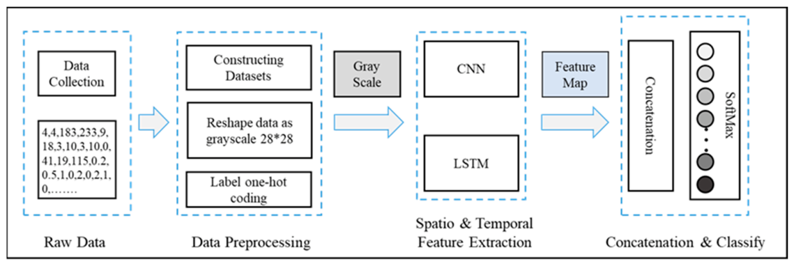
The diagnostic pipeline comprises five distinct phases: (i) multi-source telemetry acquisition, where heterogeneous sensor streams are archived; (ii) synchronized preprocessing, involving normalization and temporal alignment; (iii) spatial encoding, utilizing CNN kernels to distill inter-channel feature maps; (iv) recursive temporal mapping, where LSTM units interpret the evolution of the state space; and (v) latent fusion, terminating in a Softmax layer for multi-class anomaly isolation (Figure 2).

3.2. Industrial Data Acquisition and Physics-Informed Synthesis

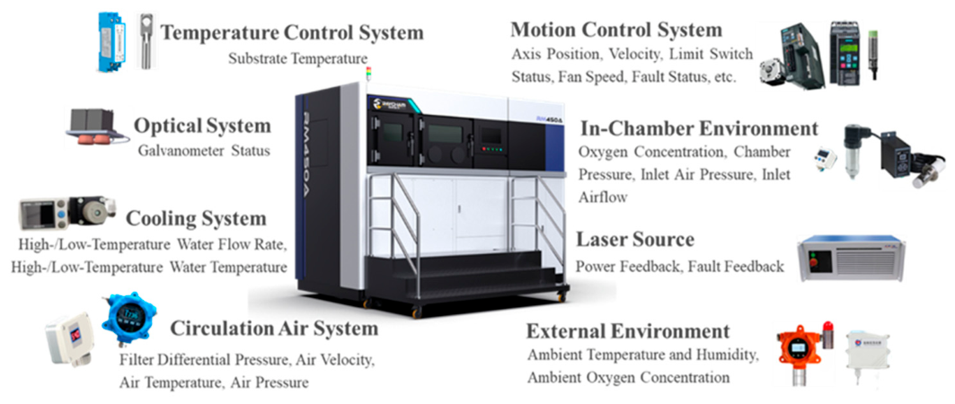
The empirical foundation of this study is derived from the RM450A industrial-grade SLM system, equipped with a comprehensive sensor array spanning seven critical functional modules (Figure 3). Data transmission is facilitated via a unified fieldbus architecture, ensuring microsecond-level synchronization across 41 monitored parameters.

3.2.1. Baseline Steady-State Data

Under nominal operating conditions, a high-fidelity baseline was established by continuously monitoring 8582 printing layers. At a deterministic sampling frequency of 1 Hz, over 290,000 multivariate records were captured. To ensure replicability and establish a rigorous physical baseline, the nominal process parameters during the steady-state data acquisition were strictly controlled. The feedstock material utilized was a commercial aluminum alloy (AlSi10Mg) consisting of highly spherical powder with a particle size distribution of 15–53 μm, processed under a continuous high-purity argon shielding gas flow. The target build geometry was a complex shoe mold.

The optical system was configured with a nominal laser power of 365 W, a focal spot diameter of 80 μm, and an average scanning speed of 1180 mm/s. The mechanical forming system was set to deposit a constant layer thickness of 40 μm.

It is critical to note the relationship between these specific process parameters and the collected multi-system telemetry. The equipment’s operational parameters directly reflect the physical regulatory effects of the chosen process settings. For different materials or build geometries, operators only need to fine-tune the process parameters, which consequently establishes a new nominal equilibrium for the equipment’s telemetry. Therefore, the proposed monitoring framework exhibits strong transferability across varying manufacturing scenarios; it functions by learning the specific healthy baseline of a given material-process envelope and detecting systemic mechanical or environmental deviations from that established equilibrium.

The baseline steady-state data reflect a statistically significant representation of the machine’s “healthy” dynamic envelope. The feature distribution across the SLM subsystems is detailed in

Table 1. The feature distribution across the SLM subsystems.

Subsystem	Component	Key Parameters (Variables)
Optical	Galvanometer	Voltage, Temperature, Humidity, Head Temperature
Cooling	High-Temperature Water	Temperature, Flow Rate
	Low-Temperature Water	Temperature, Flow Rate
Forming	Build Cylinder	Current Position, Current Velocity,
		Right-Side Position, Torque
	Recoater Blade	Current Position, Current Velocity
	Powder Delivery	Feed Multiplier, Weight
Sealing	Processing Chamber	Pressure, Oxygen Concentration 1, 2
	Main Circuit	Inlet Air Velocity, Pressure, Temperature
		Return Air Velocity, Pressure, Temperature
	Branch Circuit	Return Air Velocity, Pressure, Temperature
Preheating	Substrate Plate	Temperature (Zones 1, 2, 3)
Filtration	Pressure	Total Inlet Air, Backblow Air, Compressed Air
	Inlet Air Flow	Rear Panel, Main Chamber, Protective Window
	Differential Pressure	Coarse Filter 1, 2
Energy	Lasers	Actual Power (Laser 1, 2)

.

While the 41 monitored variables represent macro-level machine telemetry, their deviations are inextricably linked to micro-scale metallurgical defects through three primary causal pathways:

Opto-Thermal Linkage (Optical & Energy Systems): Drifts in galvanometer temperature or voltage inevitably induce focal shifts or fluctuations in scanning velocity. These deviations alter the localized Volumetric Energy Density (VED) at the powder bed, serving as direct precursors to lack of fusion (underheating) or keyhole-induced porosity (overheating).

Powder-Bed Kinematics (Forming System): Mechanical anomalies, such as abnormal recoater blade torque or positional deviations, compromise the uniformity of the powder layer. Localized excessive powder thickness prevents adequate laser penetration, reliably leading to interlayer delamination and structural weak points.

Atmospheric & Filtration Dynamics (Sealing & Filtration Systems): The stability of the shielding gas flow is heavily dependent on chamber pressure and filtration differential pressure. Subsystem deviations in these areas disrupt the laminar flow, preventing the efficient removal of spatter and condensates. The subsequent redeposition of these byproducts onto the melt-pool trajectory may directly lead to slag inclusions and severe oxidation.

By monitoring these specific telemetry channels, the proposed framework does not merely detect generic machine noise but rather isolates the systemic subsystem deviations that threaten equipment stability, moving away from predicting downstream build defects to focus strictly on machine-condition degradation.

3.2.2. Controlled Anomaly Injection via Physics-Informed Paradigms

To overcome the inherent scarcity of real-world failure labels and support categorical balance, we employed a physics-informed fault injection strategy. Controlled hardware and software overrides—executed directly via the overarching Programmable Logic Controller (PLC) interfaces, analog signal generators, and mechanical valve throttling—were utilized to synthesize reproducible degradation patterns across all seven functional modules. For instance, fluidic and thermodynamic anomalies (such as cooling or filtration issues) were primarily induced via physical valve restriction to mimic progressive occlusion, whereas electromechanical and optical drifts were synthesized by overriding the nominal setpoints within the PLC control loops. The specific manifestations across the modules include:

Optical System: Controlled perturbations were injected into the galvanometer control loops, including stochastic transients (circuit surges) and monotonic linear drifts (thermally induced deviation). A $\pm$5 °C thermal bias was also introduced to simulate opto-thermal coupling faults.

Filtration System: Harmonic pressure oscillations (0.1–0.5 MPa) were induced to emulate pump degradation, and non-linear impedance escalation was applied to represent progressive filter occlusion.

Cooling System: Flow-rate anomalies were synthesized by mechanically throttling the high-temperature and low-temperature water valves, simulating chiller flow restrictions and cooling degradation.

Forming System: Transient positional deviations and artificial torque resistance were applied to the recoater blade’s servo-drive, accurately simulating the mechanical drag caused by powder jamming or rail friction.

Sealing System: Transient oxygen concentration spikes and chamber pressure drops were induced by briefly overriding the purge gas circuitry, simulating dynamic seal leaks during the build process.

Preheating System: Asymmetric thermal gradients were created by systematically deactivating individual substrate heating channels or introducing thermal bias, replicating the failure of resistive heating elements.

Energy System: A progressive linear attenuation was applied to the actual laser output power via the overarching control system, effectively simulating the energy degradation caused by protective window contamination.

All anomalous streams were timestamp-aligned with the baseline telemetry, ensuring a standardized input tensor. Crucially, because this framework is architected for machine-condition monitoring rather than post-build part inspection, the categorical labels directly correspond to these deterministic, hardware-level physical injections. This actively controlled methodology ensures absolute ground-truth validity for the machine-state labels without the need for ex situ part validation.

3.2.3. Dataset Construction Strategies

To evaluate the impact of class distribution on diagnostic robustness and mitigate potential sampling bias, we developed three distinct anomaly-augmented datasets. These strategies are architected to simulate varied industrial scenarios, ranging from feature-proportional fault distribution to perfectly balanced multi-class benchmarks:

• Feature-Weighted (FW) Strategy: Anomalous samples are allocated proportionally to the intrinsic feature dimensionality of each subsystem. It must be noted that sensor count is not inherently proportional to the actual failure likelihood. Therefore, this strategy does not aim to perfectly mirror empirical failure rates; rather, it serves as a structural baseline to evaluate how the CNN processes localized feature density and spatial imbalances within the data matrix.
• Feature-Balanced (FB) Strategy: A uniform distribution is enforced, where each subsystem contributes an equivalent number of anomaly instances. This produces a balanced categorical benchmark to evaluate the model’s unbiased discriminative power.
• Feature-Combined (FC) Strategy: A hybrid heuristic is employed, synthesizing both feature density and the empirical criticality of specific subsystems. This strategy approximates real-world operational profiles where certain critical modules (e.g., optical or energy) require higher diagnostic priority.

The detailed categorical distributions for these three benchmarks are summarized in

Table 2. Dataset construction overview.

Dataset Type	Normal	Optical	Cooling	Forming	Sealing	Preheat	Filtration	Energy
Feature-Weighted (FW)	290,220	1960	1960	3900	5840	1460	3900	980
Feature-Balanced (FB)	290,220	2857	2857	2857	2857	2857	2857	2857
Feature-Combined (FC)	290,220	2000	2000	4000	4000	2000	4000	2000

.

3.2.4. Data Preprocessing and Spatial Mapping

The raw telemetry from the SLM system is natively formatted as $1\times 41$ multivariate vectors. However, standard 1D representations often fail to preserve the latent spatial proximity between coupled sensors. To leverage the hierarchical feature extraction capabilities of CNNs, we implemented a spatial encoding transformation.

Dimensionality Augmentation: The transformation of the 41-dimensional 1D telemetry into a $28\times 28$ 2D matrix is fundamentally driven by the need to construct a topological feature map. To conform to the matrix dimensions, dimensionality augmentation is required. Crucially, rather than employing standard zero-padding, we utilized low-variance Gaussian padding, $N\left(0, 0.01\right)$. From a signal-processing perspective, zero-padding introduces sharp, high-frequency spatial boundaries that trigger edge-effect artifacts and false filter activations during deep convolution. Conversely, the Gaussian padding functions as a neutral, stationary background. It preserves the integrity of the active feature topology without generating artificial structural gradients, while concurrently serving as a stochastic regularizer that mitigates localized overfitting.

Functional Clustering: Rather than random reshuffling, features were mapped into the 2D matrix based on functional proximity. Sensors from the same subsystem (e.g., all 12 sealing parameters) were assigned to adjacent spatial coordinates. This spatial locality ensures that subsystem-specific anomalies manifest as localized activation patterns within the CNN’s receptive field. The processing steps are summarized in Algorithm 1.

Algorithm 1: Construction of a Two-Dimensional Matrix.

Input: The original data set $D$, the number of rows $m$, and the number of column $n$;

Output: The target matrix $D^{\prime }$;

1: function GenMatrix ($D, m, n$)

2: Generate a zero padding matrix $D^{\prime }$ of $m\times n$

3: for $i\times n+j\le \left|D^{\prime }\right|$ do

4:      If $\mathrm{i} \times n+\mathrm{j} \le \left|D\right|$ then

5:          $D^{\prime }\left[i, j\right]\leftarrow D\left[i\times n+j\right]$

6:      else

7:          $D^{\prime }\left[i, j\right]\leftarrow x$, where $x$ belongs to the random normal distribution

8:      End if

9: End for

10: Return $D^{\prime }$

End function

The transition from a 1D vector to a 2D structured matrix is fundamentally driven by the physical topology of the SLM equipment. One-dimensional architectures (e.g., MLPs or 1D-CNNs) inherently assume a flat feature space, which struggles to efficiently encode the multi-hop, non-linear coupling between subsystems (e.g., the interaction between optical thermal drift and chamber gas dynamics). By arranging functionally coupled sensors (e.g., sealing pressure and filtration flow) into adjacent 2D coordinates, we elevate the feature manifold. This enables the overlapping receptive fields of the 2D CNN kernels to simultaneously capture cross-system state drifts, while the low-variance Gaussian elements act as structural anchors to prevent gradient distortion.

The preprocessing logic is formalized in Algorithm 1. For the multi-class objective, state labels were mapped to an integer space $\{0, 1, \dots , 7\}$, where 0 represents the nominal baseline, and 1–7 denote discrete subsystem failures. These labels were subsequently transformed via one-hot encoding to facilitate the final Softmax optimization, with representative data instances listed in

Table 3. One-hot encoding results.

No.	Feature Types	One-Hot Code
0	Normal	00000001
1	Optical	00000010
2	Cooling	00000100
3	Forming	00001000
4	Sealing	00010000
5	Preheat	00100000
6	Filtration	01000000
7	Energy	10000000

.

3.3. Spatiotemporal Fusion Architecture

To resolve the intricate interplay between instantaneous state transients and protracted temporal drifts across SLM subsystems, this study proposes a dual-branch spatiotemporal fusion network. The architecture is engineered to perform end-to-end representation learning by coupling a CNN for hierarchical spatial encoding with an LSTM network for recursive sequential modeling. The integrated diagnostic flow is formalized in Algorithm 2 [26].

Algorithm 2: Deep Spatiotemporal Anomaly Detection Model.

Input: The data matrix $D^{\prime }$

Output: Target model for Status-Connection Features of payload;

Step 1. Create CNN model:

Reshape input

for $i$ in range (2) do

Create convolution layer named conv_i

Set $c_i$ filter of size $s_i$

Set activation as ReLUs

Add maxpooling layer of size $p_i$

End for

Create a dropout layer with rate = 0.5

Create convolution layer named conv_3 with activation ReLU

Add global maxpooling layer, the output of which is a temp vector $V_1$

Step 2. Create LSTM model:

Create LSTM layer with $l_1$ units, with dropout $d_2$

Create a Dense layer with activation ReLU and dropout $d_3$, the output of Which

is a temp vector $V_2$

Step 3. Concatenate two model:

$V_3$ = np.concatenate($V_1$, $V_2$)

Create a full connection Dense layer with activation ReLU and dropout $d_4$

Step 4. Compile and validate model:

Set optimizer as Adam

Set loss as categorical_crossentropy

Step 5. Evaluate model:

Summary target model and Test it by evaluate data sets

Return model

3.3.1. Spatial Encoding Branch

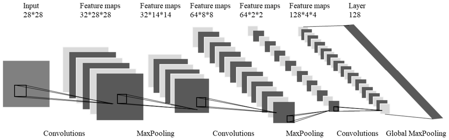
The CNN module is architected to distill localized spatial correlations from the augmented sensor matrix. By convolving across functional clusters, the module identifies subsystem-level anomaly signatures. As illustrated in Figure 4, the structured $28 \times 28$ input matrix undergoes a series of transformations to yield a 128-dimensional spatial embedding.

Let $X_{CNN}=x_1,x_2,\dots ,x_n$ denote the input sequence. For the $l$-th convolutional layer with kernel weights $W_l\in R^{k\times D\times C_l}$ and bias $b_l\in R^{C_l}$, the output feature map $F_l$ is defined as follows:

$$F_l\left(i,j,c\right)=\sigma \left(\sum _{d=1}^D\sum _{m=1}^k\left[W_l\left(m,d,c\right)\cdot X_{CNN}\left(t-m+1,d\right)\right]+b_l\left(c\right)\right)$$

(1)

where $\sigma \left(\cdot \right)$ denotes the Rectified Linear Unit (ReLU) activation function, $\mathrm{ReLU}\left(z\right)=\max \left(0,z\right)$. To enhance translation invariance and reduce computational redundancy, a max-pooling operation with window size s is applied:

$$F_{pool}\left(i,j,c\right)=\underset{t\in \mathrm{window}\left(i,j\right)}{\max }{F}_l\left(t,j,c\right)$$

(2)

The CNN branch effectively compresses the high-dimensional telemetry into a compact spatial manifold, providing a foundation for subsequent temporal reasoning.

3.3.2. Temporal Evolution Branch

Simultaneously, the LSTM branch captures the long-range dependencies inherent in the sensor sequence $X\in R^{N\times D}$. To maintain temporal continuity, a sliding-window segmentation generates input samples:

$$W_i=\left[x_{i-\left(T-1\right)},x_{i-\left(T-2\right)},\dots ,x_i\right]\in R^{T\times D}$$

(3)

The optimal temporal horizon T is not arbitrarily assigned; instead, it is determined via mutual information (MI) to ensure the window encapsulates sufficient dynamic information:

$$T=\arg \underset{\tau }{\max }\left({\displaystyle \frac{1}{\tau }}\sum _{k=1}^{\tau }\mathrm{MI}\left(x_t,x_{t-k}\right)>\theta \right)$$

(4)

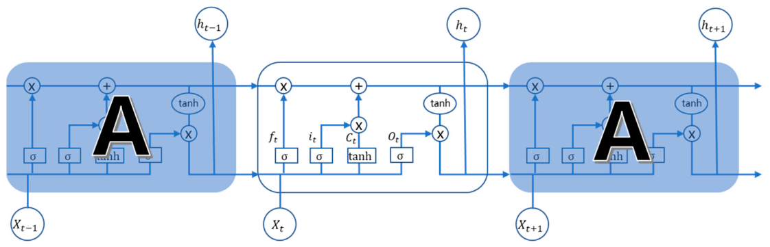
The MI was estimated utilizing Shannon entropy across 10 discrete bins to capture non-linear temporal dependencies. Based on the MI decay trajectory, the threshold $\theta = 0.25$ yielded an optimal temporal horizon of $T = 10$ s. Consequently, the sliding window segmentation was executed with a window length of 10 and a stride length of 1, applied uniformly across all nominal and anomalous data streams to standardize the temporal receptive field. To facilitate gradient flow in deep stacks and mitigate the vanishing gradient problem, residual connections are integrated between LSTM layers. This design ensures stable training while capturing the non-stationary evolution of SLM process states (Figure 5).

3.3.3. Feature Fusion and Anomaly Classification

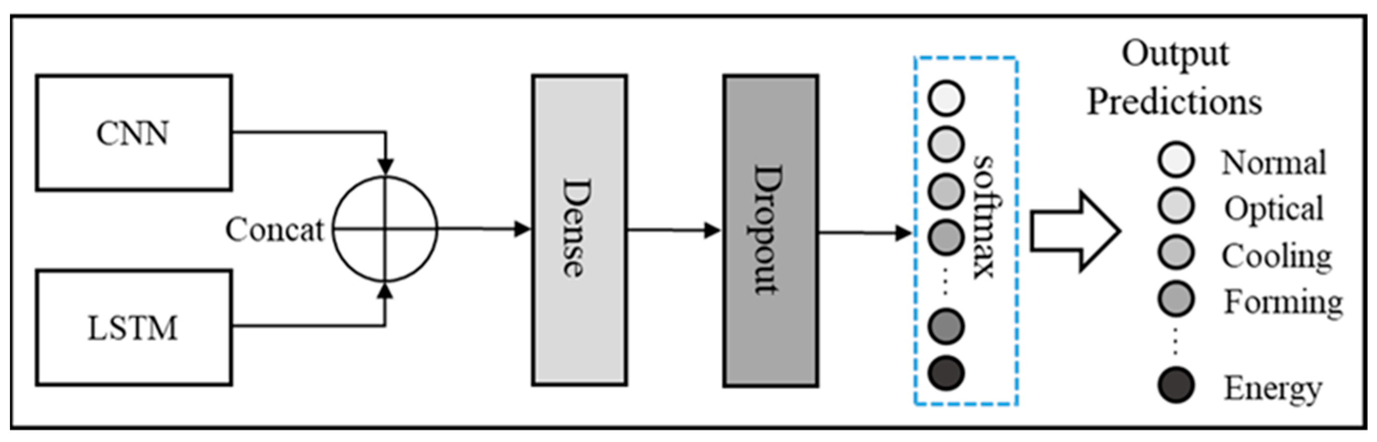
The latent representations from the dual branches—the flattened spatial feature $F_{flat}\in R^{1\times \left(T/2\times 128\right)}$ and the final temporal hidden state $h_{final}\in R^{1\times 128}$—are concatenated into a unified spatiotemporal vector $Z$:

$$Z=F_{flat}\oplus h_{final}$$

(5)

This fused vector provides a holistic snapshot of the equipment’s operational status. A final fully connected layer with parameters $W_{fc}$ maps this vector to the label space via a Softmax function:

$$Y_{pred}=Softmax\left(W_{fc}^{T}Z+b_{fc}\right)$$

(6)

The model is optimized using the categorical cross-entropy loss function $\mathcal{L}$ over $N$ training samples and C anomaly categories:

$$\mathcal{L}=-{\displaystyle \frac{1}{N}}\sum _{n=1}^N\sum _{c=1}^C{Y}_{true}^{\left(n,c\right)}\log \left(Y_{pred}^{\left(n,c\right)}\right)$$

(7)

The integrated fusion and classification pipeline is visualized in Figure 6.

3.4. Model Training and Evaluation Protocol

To systematically evaluate the diagnostic fidelity and robustness of the proposed framework, we established a benchmarking suite encompassing varying architectural depths and a standardized optimization pipeline.

3.4.1. Architectural Sensitivity Configurations

To elucidate the influence of model depth on spatiotemporal feature extraction, six architectural variants were developed. These configurations systematically scale the spatial receptive fields (CNN layers) and temporal recursion depth (LSTM layers) to identify the optimal balance between representation capacity and computational efficiency:

Shallow Architectures ($CNN \times 1$): combining a single convolutional layer (32 filters) with one or two LSTM layers (128 units each) to establish a baseline for low-complexity feature mapping;

Intermediate Architectures ($CNN \times 2$): utilizing a hierarchical spatial encoder (32 $\to$ 64 filters) to capture multi-scale subsystem correlations before sequential modeling;

Deep Architectures ($CNN \times 3$): employing a deep spatial pipeline (32 $\to$ 64 $\to$ 128 filters) designed to distill high-level abstract representations of complex industrial anomalies.

By traversing this configuration matrix, the study provides a granular analysis of how spatial extraction granularity interacts with temporal modeling depth in the SLM domain.

3.4.2. Optimization and Hyperparameter Tuning

To ensure an equitable comparison and facilitate reproducible results, a unified training protocol was enforced across all model variants. The optimization objectives and hyperparameter settings are defined as follows:

Optimization Engine: The Adam optimizer was employed with a deterministic learning rate $\eta = 0.001$ and momentum parameters ${\beta }_1=0.9,{\beta }_2=0.999$, ensuring efficient convergence across the heterogeneous fault datasets.

Regularization and Generalization: To mitigate the risk of overfitting in higher-dimensional configurations (e.g.,$CNN \times 3$), we integrated a dual-regularization strategy. This includes a dropout rate of $p = 0.5$ in the fully connected layers and $L_2$ weight decay ($\lambda = 0.001$) applied to the convolutional kernels.

Stability Mechanisms: Residual connections were implemented in multi-stack LSTM variants to stabilize gradient backpropagation through time.

Convergence Criterion: An early-stopping mechanism was adopted, where training is terminated if the validation F1 score exhibits no improvement for five consecutive epochs, thereby preventing over-optimization on the training manifold.

This standardized protocol supports that performance variances are attributable to architectural differences rather than optimization stochasticity, providing a robust foundation for the subsequent experimental analysis.

4. Experiments and Analysis

4.1. Experimental Setup and Implementation

To ensure high-fidelity training and evaluation, all computational tasks were executed on a high-performance workstation (Lenovo Group, Beijing, China: Intel^® Core™ i9-13900K, NVIDIA RTX 4090 24 GB, 64 GB DDR5 RAM). The framework was implemented using TensorFlow 2.14 and the Keras 2.3.0 ecosystem under Python 3.10. GPU-accelerated backpropagation was employed to maintain computational throughput, with convergence trajectories monitored via TensorBoard on VSCode (v1.106)

4.2. Dataset Partitioning and Preprocessing

The empirical validation relies on three strategically synthesized datasets: Feature-Weighted (FW), Feature-Balanced (FB), and Feature-Combined (FC). As detailed in Section 3, these datasets encapsulate 290,220 nominal measurements alongside seven categories of physics-informed anomalies. To preserve the spatiotemporal integrity of the sensor streams, the $1 \times 41$ vectors were transformed into $28 \times 28$ structured matrices. To rigorously prevent data leakage—a common pitfall where overlapping sliding windows artificially inflate performance—we strictly avoided stochastic (random) splitting. Instead, the continuous data streams were partitioned using a chronological block split of 70:15:15. To clarify the structural transformation from raw telemetry to model-ready inputs, the raw dataset consists of continuous 1D vectors. Following the spatial encoding ($28 \times 28$ matrix) and the sliding window segmentation (temporal horizon $T=10$, stride = 1), each discrete training sample is structured as a 3D spatiotemporal tensor of shape (10,28,28). Consequently, the chronological block split (70:15:15) was applied to these sequential blocks, ensuring that the model processes continuous time steps representing 10 s operational windows rather than isolated data points. Specifically, the temporal sequences were divided based on the actual build timeline (e.g., the first 70% of the printing layers for training, followed by 15% for validation, and the final 15% for testing). The sliding window extraction was executed strictly after this chronological partitioning, ensuring absolute zero temporal overlap between the respective datasets and guaranteeing a realistic evaluation of the model’s forward-predictive capability.

4.3. Evaluation Metrics

The diagnostic efficacy of the proposed architectures was quantified using accuracy (ACC), detection rate (DR), and false alarm rate (FAR). Furthermore, to rigorously address the highly imbalanced nature of the multi-class dataset, we evaluated the macro-precision, macro-recall, and macro-F1 scores based on the resulting confusion matrix. While ACC provides a global measure of classification fidelity, macro-F1 and FAR are critical to ensure that the model generalizes robustly across minority fault classes rather than merely overfitting to the dominant nominal state.

4.4. Architectural Comparative Analysis

To systematically investigate the influence of network depth on diagnostic performance, six structural variants were constructed via a combinatorial progression. These models differ specifically in their spatial feature extraction depth (number of CNN blocks) and temporal memory depth (number of LSTM layers). The configurations are explicitly defined as follows:

Model 1: $CNN \times 1 + LSTM \times 1$ (shallow spatial, shallow temporal);

Model 2: $CNN \times 1 + LSTM \times 2$ (shallow spatial, deep temporal);

Model 3: $CNN \times 2 + LSTM \times 1$ (medium spatial, shallow temporal);

Model 4: $CNN \times 2 + LSTM \times 2$ (medium spatial, deep temporal);

Model 5: $CNN \times 3 + LSTM \times 1$ (proposed optimal);

Model 6: $CNN \times 3 + LSTM \times 2$ (deep spatial, deep temporal).

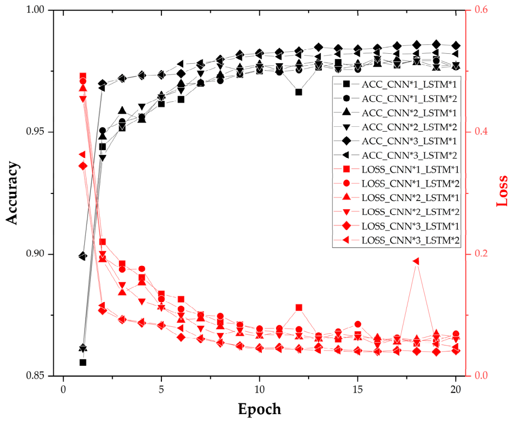
We first conducted a sensitivity analysis on the six candidate architectures using the FB dataset. As illustrated in the training trajectories (Figure 7), all models exhibited stable convergence; however, Model 5 $\left(CNN \times 3 + LSTM \times 1\right)$ demonstrated superior performance, yielding the lowest categorical cross-entropy loss and the most stable validation accuracy, where ACC denotes the classification accuracy and LOSS represents the cross-entropy loss during the training/validation phases.

The superiority of Model 5 suggests that for the high-dimensional telemetry of SLM equipment, a deeper spatial encoder (3-layer CNN) is more effective at distilling inter-system correlations than increasing the temporal recursion depth. The detailed configuration of this optimal architecture, which terminates in a 128-dimensional latent fusion layer, is formalized in

Table 4. Architecture of Model 5.

Layer	Type	Filters/Neurons	Stride
1	convolution layer	32	1
2	pooling layer	2	2
3	convolution layer	64	(2, 2)
4	pooling layer	2	(3, 3)
5	convolution layer	128	(1, 1)
6	global pooling layer	1	Default
7	LSTM	128	Default
8	full connection	1024	——
9	full connection	1024	——
10	Softmax	——	——

.

4.5. Diagnostic Performance and Discussion

4.5.1. Model Performance Analysis

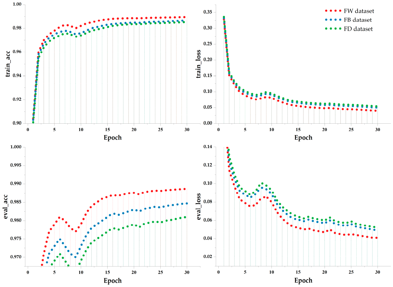
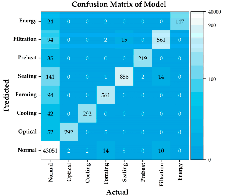
To further refine the diagnostic capability, Model 5 was subjected to extended training across the three data strategies. As shown in Figure 8, the FW dataset yielded the most robust results. Under this configuration, the model achieved a remarkable overall accuracy of 98.81% and a detection rate of 98.27%.

The confusion matrix (Figure 9) and categorical metrics (

Table 5. Model testing results.

Data Type	ACC	Precision	DR (Recall)	FAR	F1 Score
Normal	0.9889	0.9992	0.9889	0.0110	0.9941
Optical	0.9987	0.8367	0.9932	0.0012	0.9082
Cooling	0.9991	0.8743	0.9932	0.0009	0.9299
Forming	0.9975	0.8565	0.9590	0.0020	0.9048
Sealing	0.9962	0.8442	0.9772	0.0035	0.9058
Preheat	0.9992	0.8622	0.9910	0.0008	0.9221
Filtration	0.9971	0.8348	0.9590	0.0024	0.8926
Energy	0.9994	0.8497	1	0.0006	0.9187
Total (Macro)	0.9881	0.8697	0.9827	0.0028	0.9220

) reveal that the framework excels in isolating anomalies across all seven subsystems. Notably, the model maintained a high precision even in subsystems with subtle signal deviations, such as the sealing and preheating modules. The robust diagonal distribution in the confusion matrix demonstrates a high macro-F1 score, confirming the model’s excellent generalization across highly imbalanced anomaly classes. The false alarm rate (FAR) was rigorously recorded at 0.28%. It is important to note that while this FAR (0.28%) is marginally higher than estimates derived from initial stochastic-split evaluations (which often suffer from temporal data leakage), this value strictly represents the true forward-predictive FAR under chronological block splitting. This negligible rate is primarily attributed to transient boundary ‘noise’ inherent in high-frequency SLM sensors, validating that the framework does not artificially deflate error rates by memorizing correlated temporal windows.

4.5.2. Ablation Study on Spatial Encoding Topologies

To validate the structural necessity of the 2D functional layout, an ablation study was conducted comparing the proposed architecture against alternative encoding paradigms. The models were evaluated on the FB dataset.

Baseline 1 (1D-CNN-LSTM): ingesting the raw 1D vector directly, yielding an accuracy of 96.8%;

Baseline 2 (2D CNN-LSTM with Random Layout): utilizing the 28 × 28 matrix, but with the 41 features stochastically scattered, yielding an accuracy of 98.1%;

Proposed (2D CNN-LSTM with Functional Layout): grouping coupled subsystems adjacently, achieving a peak accuracy of 98.81%.

The notable performance degradation in Baseline 1 confirms that flat 1D vectors lack the spatial dimensionality required to resolve complex inter-system coupling. Furthermore, the 0.71% accuracy margin between the functional layout and the random layout empirically validates that the 2D CNN is not merely exploiting synthetic padding but is genuinely decoding the physical cross-system interactions embedded within the designed spatial topography.

While this 0.71% numerical performance gain may appear globally modest, its engineering significance is substantial. Deep CNNs possess inherent translation invariance, allowing them to eventually identify abstract correlations even within stochastically scattered inputs. However, the proposed functional layout deterministically aligns physically coupled subsystems directly within the initial receptive fields of the convolutional kernels. Given the overwhelming dominance of nominal samples in industrial operations, this sub-one-percent global improvement translates to a highly concentrated optimization at the anomaly decision boundaries. It specifically minimizes the false alarm rate (FAR) and supports the correct diagnosis of complex, long-tail multi-system faults—both of which are critical prerequisites for reliable industrial condition monitoring.

4.5.3. Performance Comparison with External Baselines

To rigorously validate the superiority of the proposed framework beyond internal depth variations, we benchmarked the optimal $CNN \times 3 + LSTM \times 1$ model against three widely adopted condition-monitoring algorithms: Random Forest (RF), representing traditional ensemble learning; 1D-CNN, serving as a purely spatial deep learning baseline; and Gated Recurrent Unit (GRU), serving as a purely temporal baseline. All models were trained and evaluated on the chronologically partitioned Feature-Weighted dataset.

The empirical results demonstrate that the RF model struggles with the high-dimensional non-linear coupling, yielding an accuracy of only 91.2%. The 1D-CNN (94.5%) and GRU (95.1%) models, which operate directly on the original sequential and tabular structures, respectively, show improvement but suffer from higher false alarm rates (FARs). The fundamental limitation of 1D-CNNs is their linear receptive field, which restricts kernel operations to sequential neighbors and fails to model complex inter-system coupling. By transforming the data into a 2D matrix, our 2D kernels simultaneously capture cross-domain physics (e.g., thermal and pneumatic coupling) across functionally adjacent nodes. This topological advantage explains why single-domain baseline models fail to adequately process spatial channel correlations alongside temporal evolution. In contrast, the proposed 2D CNN-LSTM achieves a superior accuracy of 98.8% with an exceptionally low FAR. This comparative analysis definitively confirms that the synergistic spatiotemporal fusion is indispensable for accurately decoupling the complex physical signatures of SLM equipment.

4.5.4. Computational Efficiency and Real-Time Feasibility

In industrial SLM deployments, diagnostic models must execute strictly within the equipment’s control cycle to enable predictive interventions. To validate real-time applicability, the inference latency of the trained $CNN \times 3 + LSTM \times 1$ model was empirically quantified.

During the testing phase, the average processing time required to encode and classify a single temporal window (comprising 10 timesteps of $28 \times 28$ structured matrices) was recorded at 4.2 milliseconds per sample. Given that the underlying machine telemetry is generated at a frequency of 1 Hz (imposing a maximum allowable latency budget of 1000 ms), the model’s inference consumes merely 0.42% of the available temporal cycle. This substantial computational buffer guarantees that the framework can be deployed for synchronous, on-the-edge condition monitoring without bottlenecking the machine’s primary Programmable Logic Controller (PLC) network.

4.6. Feature Space Visualization via t-SNE

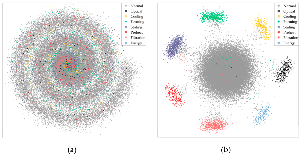
To investigate the discriminative power of the learned spatiotemporal representations, we employed t-Distributed Stochastic Neighbor Embedding (t-SNE) to project the high-dimensional latent space into a 2D plane.

As visualized in Figure 10, the nominal operational state forms a dense, centrally located cluster, whereas the seven anomaly categories manifest as distinct, well-separated peripheral clusters. The clear inter-class margins and high intra-class density suggest that the hybrid CNN-LSTM architecture effectively extracts linearly separable latent features from the highly coupled telemetry. While this 2D qualitative embedding cannot be interpreted as conclusive proof that the model has learned the absolute physical manifold of the SLM process, it serves as strong supportive evidence of the network’s discriminative capacity. It visually demonstrates that the framework translates raw operational noise into highly separable diagnostic clusters, thereby supporting its reliability for downstream classification tasks.

4.7. Summary

The experimental results confirm that the $CNN \times 3 + LSTM \times 1$ configuration, coupled with a feature-weighted data strategy, provides an optimal solution for SLM anomaly detection. The framework’s ability to achieve near-perfect accuracy while maintaining high separability in the feature space demonstrates its potential for real-time industrial monitoring and predictive maintenance.

5. Conclusions and Discussion

The industrial maturation of Selective Laser Melting is increasingly contingent upon the ability to perform robust machine-condition monitoring and classify subsystem faults within its highly coupled, multi-system operational fabric. This study has developed and validated a deep spatiotemporal framework that transcends the limitations of traditional univariate monitoring by synergistically coupling CNN-based spatial encoders with LSTM-based temporal decoders.

The core synthesis of our findings and their implications for the field are as follows:

• System-Level Diagnostic Fidelity: Through the physics-informed synthesis of anomalies across seven critical subsystems, we demonstrated that the Feature-Weighted (FW) data strategy most accurately reflects the stochastic nature of SLM failures. By aligning the diagnostic resolution with the sensory dimensionality of each module, the framework facilitates balanced sensitivity across the entire equipment architecture.
• Architectural Optimization: Our comparative analysis of six deep learning topologies reveals a critical design paradigm for SLM monitoring: spatial depth outweighs temporal recursion. The superior performance of the $CNN \times 3 + LSTM \times 1$ configuration suggests that distilling high-dimensional inter-subsystem correlations is more vital for fault isolation than modeling excessively long-range temporal sequences, which can introduce noise and gradient instability.
• Empirical Performance and Separability: Achieving an overall accuracy of 98.8%, the proposed model establishes a high-fidelity benchmark for real-time diagnostics. The t-SNE manifold visualization provides conclusive evidence that the network effectively transforms raw, noisy telemetry into a structured feature space where normal baselines and multi-class anomalies are linearly separable, thereby enhancing the reliability of autonomous decision-making in production environments.
• Operational Implications: Beyond numerical accuracy, this research provides a scalable technical roadmap for the transition from reactive to predictive maintenance in metal additive manufacturing. The framework’s ability to isolate faults at the subsystem level provides actionable intelligence for targeted hardware interventions. By enabling preemptive machine adjustments before mechanical deviations escalate, it strongly supports predictive maintenance protocols.

Limitations and Future Perspectives

While the proposed framework demonstrates exceptional diagnostic fidelity, it inherently relies on a supervised learning paradigm, which necessitates the acquisition of labeled anomalous data. In authentic industrial deployments, catastrophic SLM failures are relatively rare, leading to highly imbalanced datasets. Therefore, a critical limitation of the current study is its dependence on physics-informed fault injection rather than naturally occurring degradation over years of operation. Future deployment must explore the transition toward semi-supervised or fully unsupervised frameworks. Furthermore, while our chronological split demonstrates that the model does not merely memorize repeated build-specific patterns within the same geometry, evaluating the transferability of these learned spatiotemporal embeddings across entirely different SLM platforms and novel component geometries will be essential for creating generalized, fleet-wide predictive maintenance solutions.

References

1. Soni, N.; Renna, G.; Leo, P. Advancements in metal processing additive technologies: Selective laser melting (SLM). Metals 2024, 14, 1081. [Google Scholar] [CrossRef]
2. Li, Z.; Zhu, Y.; Cao, R. The state of the art in defect monitoring technologies for selective laser melting processes. 3D Print. Addit. Manuf. 2025. [Google Scholar] [CrossRef]
3. Fang, Q.; Xiong, G.; Zhou, M.C.; Tamir, T.S.; Yan, C.B.; Wu, H.; Shen, Z.; Wang, F.Y. Process monitoring, diagnosis and control of additive manufacturing. IEEE Trans. Autom. Sci. Eng. 2022, 21, 1041–1067. [Google Scholar] [CrossRef]
4. Wang, L.; Xing, F.; Shi, J.; Wang, Q. Dual-model fusion method based on DBTBoost for fault diagnosis. IEEE Trans. Instrum. Meas. 2025, 74, 3535210. [Google Scholar] [CrossRef]
5. Zeiser, A.; Özcan, B.; Kracke, C.; van Stein, B.; Bäck, T. A data-centric approach to anomaly detection in layer-based additive manufacturing. at-Automatisierungstechnik 2023, 71, 81–89. [Google Scholar] [CrossRef]
6. Zamiela, C.E. Enhancing Data-Driven Process Quality Control in Metal Additive Manufacturing: Sensor Fusion, Physical Knowledge Integration, and Anomaly Detection. Ph.D. Dissertation, Mississippi State University, Starkville, MS, USA, 2024. Available online: https://scholarsjunction.msstate.edu/td/6211/ (accessed on 11 December 2025).
7. Wu, H.; Yu, Z.; Wang, Y. Experimental study of the process failure diagnosis in additive manufacturing based on acoustic emission. Measurement 2019, 136, 445–453. [Google Scholar] [CrossRef]
8. Bhattacharya, M.; Penica, M.; O’Connell, E.; Hayes, M. AI-driven real-time failure detection in additive manufacturing. Procedia Comput. Sci. 2024, 232, 3229–3238. [Google Scholar] [CrossRef]
9. Sampedro, G.A.R.; Rachmawati, S.M.; Kim, D.S.; Lee, J.M. Exploring machine learning-based fault monitoring for polymer-based additive manufacturing: Challenges and opportunities. Sensors 2022, 22, 9446. [Google Scholar] [CrossRef]
10. Chen, L.; Bi, G.; Yao, X.; Su, J.; Tan, C.; Feng, W.; Benakis, M.; Chew, Y.; Moon, S.K. In-situ process monitoring and adaptive quality enhancement in laser additive manufacturing: A critical review. J. Manuf. Syst. 2024, 74, 527–574. [Google Scholar] [CrossRef]
11. Xie, M.; Shi, Z.; Yue, X.; Ding, M.; Qiu, Y.; Jia, Y.; Li, B.; Li, N. Fault diagnosis and prediction system for metal wire feeding additive manufacturing. Sensors 2024, 24, 4277. [Google Scholar] [CrossRef]
12. Guo, Y.; Zhang, Y.; Pan, Z.; Shen, L.; Lu, X. Recent progress of sensing and machine learning technologies for process monitoring and defects detection in wire arc additive manufacturing. J. Manuf. Process. 2024, 125, 489–511. [Google Scholar] [CrossRef]
13. Zamanzadeh Darban, Z.; Webb, G.I.; Pan, S.; Salehi, M. Deep learning for time series anomaly detection: A survey. ACM Comput. Surv. 2024, 57, 15. [Google Scholar] [CrossRef]
14. Elnakib, O.; Shaaban, E.; Mahmoud, M.; Emara, K. EIDM: Deep learning model for IoT intrusion detection systems. J. Supercomput. 2023, 79, 13243–13271. [Google Scholar] [CrossRef]
15. Esmaeili, F.; Cassie, E.; Nguyen, H.P.T.; Plank, N.O.V.; Unsworth, C.P.; Wang, A. Anomaly detection for sensor signals utilizing deep learning autoencoder-based neural networks. Bioengineering 2023, 10, 405. [Google Scholar] [CrossRef] [PubMed]
16. Li, G.; Jung, J.J. Deep learning for anomaly detection in multivariate time series: Approaches, applications, and challenges. Inf. Fusion 2023, 91, 93–102. [Google Scholar] [CrossRef]
17. Chung, J.; Shen, B.; Kong, Z.J. Anomaly detection in additive manufacturing processes using supervised classification with imbalanced sensor data based on generative adversarial network. J. Intell. Manuf. 2024, 35, 2387–2406. [Google Scholar] [CrossRef]
18. Zeiser, A.; Özcan, B.; van Stein, B.; Bäck, T. Evaluation of deep unsupervised anomaly detection methods with a data-centric approach for on-line inspection. Comput. Ind. 2023, 146, 103852. [Google Scholar] [CrossRef]
19. El-Shafeiy, E.; Alsabaan, M.; Ibrahem, M.I.; Elwahsh, H. Real-time anomaly detection for water quality sensor monitoring based on multivariate deep learning technique. Sensors 2023, 23, 8613. [Google Scholar] [CrossRef]
20. Amiri, A.F.; Kichou, S.; Oudira, H.; Chouder, A.; Silvestre, S. Fault detection and diagnosis of a photovoltaic system based on deep learning using the combination of a convolutional neural network (CNN) and bidirectional gated recurrent unit (Bi-GRU). Sustainability 2024, 16, 1012. [Google Scholar] [CrossRef]
21. Zhao, S.; Duan, Y.; Roy, N.; Zhang, B. A deep learning methodology based on adaptive multiscale CNN and enhanced highway LSTM for industrial process fault diagnosis. Reliab. Eng. Syst. Saf. 2024, 249, 110208. [Google Scholar] [CrossRef]
22. Anuradha, R.; Swathi, B.; Nagpal, A.; Chaturvedi, P.; Kalra, R.; Alwan, A.A. Deep learning for anomaly detection in large-scale industrial data. In Proceedings of the 2023 10th IEEE Uttar Pradesh Section International Conference on Electrical, Electronics and Computer Engineering (UPCON), Gautam Buddha Nagar, India, 1–3 December 2023. [Google Scholar] [CrossRef]
23. Xu, H.; Lv, R.; Zi, B. A multimodal spatiotemporal fusion network with physical-data-driven learning for additive manufacturing fault diagnosis. IEEE Trans. Instrum. Meas. 2025, 74, 3566415. [Google Scholar] [CrossRef]
24. Yang, G.; Xie, Y.L.; Zhao, S.; Qin, L.; Wang, X.; Wu, B. Quality control: Internal defects formation mechanism of selective laser melting based on laser-powder-melt pool interaction: A review. Chin. J. Mech. Eng. Addit. Manuf. Front. 2022, 1, 100037. [Google Scholar] [CrossRef]
25. Wang, R.; Garcia, D.; Kamath, R.R.; Dou, C.; Ma, X.; Shen, B.; Choo, H.; Fezzaa, K.; Yu, H.Z.; Kong, Z. In situ melt pool measurements for laser powder bed fusion using multi sensing and correlation analysis. Sci. Rep. 2022, 12, 13716. [Google Scholar] [CrossRef]
26. Zhao, J.; Zeng, P.; Chen, C.; Dong, Z.; Han, J. Deep Learning Anomaly Detection Based on Hierarchical Status-Connection Features in Networked Control Systems. Intell. Autom. Soft Comput. 2021, 30, 337–350. [Google Scholar] [CrossRef]
27. Jafarbigloo, S.K.; Danyali, H. Nuclear atypia grading in breast cancer histopathological images based on CNN feature extraction and LSTM classification. CAAI Trans. Intell. Technol. 2021, 6, 426–439. [Google Scholar] [CrossRef]
Figure 1. Principle of the Selective Laser Melting process.
Coatings 16 00517 g001
Figure 2. Overall architecture of the proposed deep spatiotemporal anomaly detection model.
Coatings 16 00517 g002
Figure 3. Configuration of the RM450A SLM system.
Coatings 16 00517 g003
Figure 4. CNN module architecture.
Coatings 16 00517 g004
Figure 5. LSTM module architecture [27].
Coatings 16 00517 g005
Figure 6. Fusion and classification pipeline.
Coatings 16 00517 g006
Figure 7. Performance comparison of the six models.
Coatings 16 00517 g007
Figure 8. Performance comparison of Model 5 on the three datasets.
Coatings 16 00517 g008
Figure 9. Confusion matrix of the proposed model.
Coatings 16 00517 g009
Figure 10. Feature space visualization using t-SNE: (a) unlearned original features; (b) separated features extracted by Model 5.
Coatings 16 00517 g010