Approximate Analytical Solutions of Nonlinear Jerk Equations Using the Parameter Expansion Method

Abstract

The Parameter Expansion Method (PEM) is employed to study nonlinear Jerk equations, which are often difficult to solve because of their strong nonlinearity. This method provides higher accuracy and broader applicability, enabling analytical insights and closed-form approximations. This study explores the use of Prof. He’s PEM to derive approximate analytical solutions of the nonlinear third-order Jerk equation, this model is commonly encountered in the analysis of complex dynamical systems across physics and engineering. Owing to the strong nonlinearity inherent in Jerk equations, exact solutions are often unattainable. The PEM provides a simple, effective framework by expanding the solution with respect to an embedding parameter, allowing accurate approximations without the need of small parameters or linearization. The method’s reliability and precision are validated through comparisons with numerical simulations, demonstrating its practicality and robustness in tackling nonlinear problems. The results indicate that PEM provides highly accurate approximations of nonlinear Jerk equation, showcasing greater simplicity and efficiency relative to other analytical methods, along with excellent concordance with numerical simulations. Additionally, the nonlinear Jerk equation demonstrates exact approximate solutions via PEM, closely mirroring numerical results and surpassing several contemporary analytical techniques in efficiency and usability. Furthermore, the study indicates that PEM is a straightforward and effective approach in solving nonlinear Jerk equation. It generates accurate estimates that nearly align with numerical simulations and surpass numerous other analytical methods.

1. Introduction

Nonlinear third-order differential equations play a significant role in modeling a wide range of physical and engineering systems, particularly those involving higher-order dynamics such as Jerk (a third-order derivative of displacement), which is essential in characterizing smooth transitions in acceleration. There are several key applications of nonlinear Jerk equations across various fields, such as robotics, motion control, vehicle dynamics, biomechanics, structural engineering, plasma physics, nonlinear circuits, dynamical systems, MEMS/NEMS devices, and seismology [1,2,3]. Due to their inherent nonlinearity and higher order, exact analytical solutions of such equations are often difficult or impossible to achieve. Traditional techniques such as perturbation methods have been widely applied to solve weakly nonlinear differential equations [4]. However, their effectiveness diminishes when dealing with strongly nonlinear problems. This has motivated the development of alternative analytical and semi-analytical approaches capable of handling stronger nonlinearities without requiring small parameters. Among these, He’s PEM has emerged as a simple yet powerful analytical tool [5,6]. The PEM constructs approximate solutions by expanding the response in terms of an artificial parameter, enabling effective handling of nonlinearities with minimal computational effort.

Analytical solutions of nonlinear Jerk equations are infrequently obtainable due to the strong nonlinearity inherent in their structure. Consequently, researchers have developed various analytical and semi-analytical methods to approximate periodic solutions and analyze system dynamics [7,8,9,10]. More specifically, Wang et al. [11] applied He’s PEM to obtain analytical solutions of nonlinear Jerk equations. Hu [12] applied the Lindstedt–Poincaré perturbation method to a class of nonlinear Jerk equations, deriving approximate frequency–amplitude relations of systems with cubic nonlinearity. Similarly, Ma et al. [13] employed He’s Homotopy perturbation method (HPM) to obtain analytical approximations of Jerk oscillators, accomplishing results that agreed well with numerical simulations. In an effort to enhance flexibility and accuracy, Marinca et al. [14] introduced the optimal auxiliary functions method to tackle nonlinear Jerk systems, effectively reducing residual errors through optimally selected auxiliary terms. Hu et al. [15] proposed a modified Mickens iteration procedure to handle nonlinear Jerk equations, which demonstrated rapid convergence and accurate estimation of periodic solutions, even of strongly nonlinear cases. Ramos [16] applied the Lindstedt–Poincaré method to analyze Jerk equations. While Leung and Guo [17] applied the residue harmonic balance approach. Ismail and Abu-Zinadah [18] extend the global error minimization method to obtain analytic approximations of nonlinear Jerk equations. El-Dib [19,20] used the non-perturbative approach and Galerkin’s method, respectively, to solve the nonlinear Jerk oscillator.

More recently, Ismail and Yamani [21] presented a hybrid approach based on the Modified Iteration Method and He’s PEM, offering an efficient framework for solving complex Jerk equations without resorting to linearization or small parameter assumptions. Nonlinear Jerk equations, when examined through PEM, possess significant experimental and practical applications in science and engineering. In mechanical systems, Jerk equations are essential in creating smoother motion profiles in robotics, computer numerical control (CNC) machining, and transportation systems, as abrupt changes in acceleration can lead to wear, vibration, or discomfort. Nonlinear Jerk models in electrical engineering characterize specific chaotic oscillators and nonlinear circuits, facilitating the advancement of secure communication systems and signal processing devices. In biomechanics, Jerk is significant in modeling human or animal movement, contributing to ergonomic design, prosthetics, and sports performance analysis. The PEM improves these applications by delivering precise analytical approximations that can be empirically tested, diminishing dependence on solely numerical simulations and facilitating real-time implementation in control systems. In experimental contexts, PEM-based models facilitate parameter optimization, forecast system behavior under diverse conditions, and enhance designs for stability and performance, serving as a potent instrument in connecting theoretical nonlinear dynamics with practical breakthroughs.

The present study aims to explore the application of PEM to a class of nonlinear third-order differential equations, often referred to as Jerk equations. The focus is on deriving accurate approximate solutions and comparing them with the known results to demonstrate the method’s efficiency, reliability, and simplicity. The findings contribute to the growing body of literature on analytical methods of nonlinear systems, offering a valuable tool for researchers who working with higher-order nonlinear differential equations.

Jerk equations feature complex displacement–velocity–acceleration coupling and high-order nonlinearities that complicate their analysis. This study is very significant to demonstrate the systematic application of PEM to derive highly accurate analytical approximations of strongly nonlinear Jerk equations. The PEM solutions not only match numerical simulations with remarkable precision, but also successfully capture elusive phenomena like amplitude-dependent frequency shifts and higher-harmonic content features that often missed by traditional perturbation methods. These findings establish PEM as an efficient and reliable analytical tool in exploring Jerk equations in various engineering and physical contexts.

To crystallize the presentation of the paper, its remainder is organized as follows: Section 2 is devoted to introducing the implementation of PEM. This section involves two special cases. The results and discussion are presented in Section 3. Lastly, the conclusions are presented in Section 4.

2. Implementation of PEM

The general third-order nonlinear Jerk equation, according to Gottlieb [22], can be described as

$$\stackrel{⃛}{x}+\alpha \dot{x}+\beta {\dot{x}}^3+\gamma x^2\dot{x}-\delta x\dot{x}\ddot{x}+\mu \dot{x}{\ddot{x}}^2=0,$$

(1)

with the initial conditions of

$$x\left(0\right)=0,\hspace{1em}\dot{x}\left(0\right)=A,\hspace{1em}\ddot{x}\left(0\right)=0.$$

(2)

Equation (1) is highly versatile. It applies to mechanical vibrations, nonlinear circuits, chaos theory, control and robotics, human motion, biomechanics, and aerospace systems.

According to PEM [23,24], the solution is expanded in a series of artificial parameters, p, in the following form:

$$x=x_0+p{x}_1+p^2{x}_2+\cdots ,$$

(3)

in which the parameter $\alpha ,\beta ,\gamma ,\delta ,$ and $\mu$ can be expanded as $x$ in Equation (3):

$$\alpha ={\omega }^2+p{\omega }_1+p^2{\omega }_2+\cdots ,$$

(4)

$$\beta =p{a}_1+p^2{a}_2+\cdots ,$$

(5)

$$\gamma =p{b}_1+p^2{b}_2+\cdots ,$$

(6)

$$\delta =p{c}_1+p^2{c}_2+\cdots ,$$

(7)

$$\mu =p{d}_1+p^2{d}_2+\cdots .$$

(8)

Substituting Equations (3)–(8) into Equation (1) and equating the terms of the identical powers of p, we have

$${\stackrel{⃛}{x}}_0+{\omega }^2{\dot{x}}_0=0,$$

(9)

$${\stackrel{⃛}{x}}_1+{\omega }^2{\dot{x}}_1+b_1{\dot{x}}_0{x}_0^2+{\omega }_1{\dot{x}}_0+a_1{\dot{x}}_0^3-{c_{1}x}_0{\dot{x}}_0{\ddot{x}}_0+d_1{\dot{x}}_0{\ddot{x}}_0^2=0,$$

(10)

$$\begin{gathered} {\stackrel{⃛}{x}}_2+{\omega }^2{\dot{x}}_2+b_{1}2x_0{x}_1{\dot{x}}_0+b_2{x}_0^2{\dot{x}}_0+{\omega }_2{\dot{x}}_0+a_2{\dot{x}}_0^3+b_1{x}_0^2{\dot{x}}_1+{\omega }_1{\dot{x}}_1+3a_1{\dot{x}}_0^2{\dot{x}}_1-c_1{x}_1{\dot{x}}_0{\ddot{x}}_0-c_2{x}_0{\dot{x}}_0{\ddot{x}}_0 \\ -c_1{x}_0{\dot{x}}_0{\ddot{x}}_0+d_2{\dot{x}}_0{\ddot{x}}_0^2+d_1{\dot{x}}_1{\ddot{x}}_0^2-c_1{x}_0{\dot{x}}_0{\ddot{x}}_1+2d_2{\dot{x}}_0{\ddot{x}}_0{\ddot{x}}_1=0. \end{gathered}$$

(11)

The solution of Equation (9), in light of the initial conditions, is given as

$$x_0={\displaystyle \frac{A}{\omega }}\mathrm{s}\mathrm{i}\mathrm{n}\left(\omega t\right).$$

(12)

Substituting Equation (12) into Equation (10), then solving the results after eliminating the secular terms, we obtain the following:

$$x_1=A^3\left({\displaystyle \frac{a_1}{96{\omega }^3}}-{\displaystyle \frac{b_1}{96{\omega }^5}}+{\displaystyle \frac{c_1}{96{\omega }^3}}-{\displaystyle \frac{d_1}{96\omega }}\right)\mathrm{s}\mathrm{i}\mathrm{n}(3\omega t),$$

(13)

$${\omega }_1=-{\displaystyle \frac{A^2\left(3{\omega }^2{a}_1+b_1-{\omega }^2{c}_1+{\omega }^4{d}_1\right)}{4{\omega }^2}}.$$

(14)

Similar to the previous step, we can obtain $x_2$ and ${\omega }_2$ in the same manner:

$$\begin{gathered} x_2=\left({\displaystyle \frac{A^5{a}_1^2}{512{\omega }^5}}+{\displaystyle \frac{A^3{a}_2}{96{\omega }^3}}-{\displaystyle \frac{A^5{a}_1{b}_1}{768{\omega }^7}}-{\displaystyle \frac{A^5{b}_1^2}{1536{\omega }^9}}-{\displaystyle \frac{A^3{b}_2}{96{\omega }^5}}+{\displaystyle \frac{A^5{a}_1{c}_1}{384{\omega }^5}}+{\displaystyle \frac{A^5{c}_1^2}{1536{\omega }^5}}-{\displaystyle \frac{A^3{c}_2}{96{\omega }^3}}-{\displaystyle \frac{A^5{a}_1{d}_1}{768{\omega }^3}}-{\displaystyle \frac{A^5{b}_1{d}_1}{768{\omega }^5}}-{\displaystyle \frac{A^5{d}_1^2}{1536\omega }}-{\displaystyle \frac{A^3{d}_2}{96\omega }}+ \\ {\displaystyle \frac{A^3{a}_1{\omega }_1}{768{\omega }^5}}-{\displaystyle \frac{A^3{b}_1{\omega }_1}{768{\omega }^7}}+{\displaystyle \frac{A^3{c}_1{\omega }_1}{768{\omega }^5}}-{\displaystyle \frac{A^3{d}_1{\omega }_1}{768{\omega }^3}}\right)\mathrm{S}\mathrm{i}\mathrm{n}\left(3\omega t\right)+\left({\displaystyle \frac{A^5{a}_1^2}{5120{\omega }^5}}-{\displaystyle \frac{7A^5{a}_1{b}_1}{\mathrm{23,040}{\omega }^7}}+{\displaystyle \frac{A^5{b}_1^2}{9216{\omega }^9}}-{\displaystyle \frac{A^5{a}_1{c}_1}{\mathrm{11,520}{\omega }^5}}+{\displaystyle \frac{A^5{b}_1{c}_1}{5760{\omega }^7}}-{\displaystyle \frac{13A^5{c}_1^2}{\mathrm{46,080}{\omega }^5}}- \\ {\displaystyle \frac{A^5{a}_1{d}_1}{1536{\omega }^3}}+{\displaystyle \frac{13A^5{b}_1{d}_1}{\mathrm{23,040}{\omega }^5}}-{\displaystyle \frac{A^5{c}_1{d}_1}{5760{\omega }^3}}+{\displaystyle \frac{7A^5{d}_1^2}{\mathrm{15,360}\omega }}\right)\mathrm{s}\mathrm{i}\mathrm{n}\left(5\omega t\right). \end{gathered}$$

(15)

$$\begin{gathered} {\omega }_2={\displaystyle \frac{1}{384{\omega }^6}}{A}^2\left(-9A^2{\omega }^4{a}_1^2-288{\omega }^6{a}_2+10A^2{\omega }^2{a}_1{b}_1-A^2{b}_1^2-96{\omega }^4{b}_2-16A^2{\omega }^4{a}_1{c}_1+8A^2{\omega }^2{b}_1{c}_1 \\ -7A^2{\omega }^4{c}_1^2-96{\omega }^6{c}_2-6A^2{\omega }^6{a}_1{d}_1+14A^2{\omega }^4{b}_1{d}_1-8A^2{\omega }^6{c}_1{d}_1+15A^2{\omega }^8{d}_1^2-96{\omega }^8{d}_2\right). \end{gathered}$$

(16)

The higher-order approximate solutions to Equation (1) for $x\left(t\right)$ and $\omega$ can be established in a similar manner.

Now, we shall study some different relevant cases considering main Equation (1).

2.1. Special Case 1: Jerk Equation Based on Displacement–Velocity–Acceleration Interaction

Putting $\beta =\gamma =\mu =0$, and $\alpha =\delta =1,$ in Equation (1), we obtain the Jerk function involving displacement–velocity–acceleration product and velocity term in the following form [22]:

$$\stackrel{⃛}{x}+\dot{x}-x\dot{x}\ddot{x}=0,\hspace{1em}x\left(0\right)=0, \dot{x}\left(0\right)=A,\hspace{1em}\ddot{x}\left(0\right)=0.$$

(17)

Equation (17) describes a system where a competition between linear velocity effects and a nonlinear product of displacement, velocity, and acceleration governs the rate of change in acceleration (Jerk). This makes it a model for nonlinear oscillators with strong displacement–velocity–acceleration coupling, relevant in mechanical vibrations, nonlinear circuits, and complex dynamical systems.

Inserting Equations (3), (4) and (7) into Equation (17), a new trial function is proposed for the first-order approximation as

$${\stackrel{⃛}{x}}_0+{\omega }^2{\dot{x}}_0=0,$$

(18)

$${\stackrel{⃛}{x}}_1+{\omega }^2{\dot{x}}_1+{\omega }_1{\dot{x}}_0-c_1{x}_0{\dot{x}}_0{\ddot{x}}_0=0,$$

(19)

$${\stackrel{⃛}{x}}_2+{\omega }^2{\dot{x}}_2+{\omega }_2{\dot{x}}_0+{\omega }_1{\dot{x}}_1-c_1{x}_1{\dot{x}}_0{\ddot{x}}_0-c_2{x}_0{\dot{x}}_0{\ddot{x}}_0-c_1{x}_0{\dot{x}}_1{\ddot{x}}_1-c_1{x}_0{\dot{x}}_0{\ddot{x}}_1=0.$$

(20)

A new trial function is proposed for the first-order approximation, Equation (18), as

$$x_0(t)={\displaystyle \frac{A}{\omega }}\sin \omega t.$$

(21)

Substituting Equation (21) into Equation (19), we can write

$${\stackrel{⃛}{x}}_1+{\omega }^2{\dot{x}}_1+{\displaystyle \frac{1}{4}}(A^3{c}_1+4A{\omega }_1)\cos \left(\omega t\right)-{\displaystyle \frac{1}{4}}{A}^3{c}_1\cos \left(3\omega t\right)=0.$$

(22)

Solving the above results after eliminating the secular term, and choosing $c_1=0$ and $c_2=0,$ we obtain

$$x_1\left(t\right)=-{\displaystyle \frac{A^3}{96{\omega }^3}}\sin \left(3\omega t\right),\hspace{1em}{\omega }_1=-{\displaystyle \frac{1}{4}}{A}^2,$$

(23)

$$x_2\left(t\right)=-{\displaystyle \frac{A^5}{3072{\omega }^5}}\mathrm{s}\mathrm{i}\mathrm{n}(3\omega t)+{\displaystyle \frac{13A^5}{\mathrm{46,080}{\omega }^5}}\mathrm{s}\mathrm{i}\mathrm{n}(5\omega t),\hspace{1em}{\omega }_2={\displaystyle \frac{7A^4}{384{\omega }^2}}.$$

(24)

Applying the same procedure, we can find $x_3$, $x_4$, … and so on.

Now using Equations (21), (23) and (24), we obtain the third-order solution for $x\left(t\right),$ as follows

$$x\left(t\right)={\displaystyle \frac{A}{\omega }}\sin (\omega t)-\left({\displaystyle \frac{A^3}{96{\omega }^3}}+{\displaystyle \frac{A^5}{3072{\omega }^5}}\right)\mathrm{s}\mathrm{i}\mathrm{n}\left(3\omega t\right)+{\displaystyle \frac{13A^5}{\mathrm{46,080}{\omega }^5}}\mathrm{s}\mathrm{i}\mathrm{n}\left(5\omega t\right),$$

(25)

$$\omega ={\displaystyle \frac{1}{4}}\sqrt{8+2A^2+\sqrt{64+32A^2-{\displaystyle \frac{2A^4}{3}}}}.$$

(26)

Equations (25) and (26) represent the effects of strong nonlinearity: amplitude-dependent frequency and wave forming across higher harmonics, both of which are a direct result of the three-way feedback between $x,\dot{x},$ and $\ddot{x}$ that controls the Jerk equation. These features characterize nonlinear oscillators in mechanical systems, circuits, and elsewhere, and determine their response under different excitation amplitudes.

2.2. Special Case 2: Jerk Function, Involving the Product of Velocity and the Square of Acceleration, Along with a Term Proportional to Velocity

Putting $\beta =\gamma =\delta =0$, and $\alpha =\mu =1,$ in Equation (1), then we obtain the Jerk function involving velocity times acceleration squared, and velocity in the following form [22]:

$$\stackrel{⃛}{x}+\dot{x}+\dot{x}{\ddot{x}}^2=0,\hspace{1em}x\left(0\right)=0, \dot{x}\left(0\right)=A,\hspace{1em}\ddot{x}\left(0\right)=0.$$

(27)

Equation (27) describes a system where Jerk is governed by a balance between a linear velocity effect and a nonlinear velocity–acceleration interaction. The nonlinear term makes the system highly sensitive to bursts of acceleration: the faster and more forcefully the system accelerates, the stronger feedback on Jerk. This means that the system behaves like a dynamical amplifier of rapid motion, showing strong nonlinear resistance or amplification depending on the motion’s phase and intensity.

Following the same procedure as the previous case, after performing many calculations, we can finally obtain the general solution up to third order in the following form:

$$x\left(t\right)={\displaystyle \frac{A}{\omega }}\sin (\omega t)-({\displaystyle \frac{A^3}{96\omega }}+{\displaystyle \frac{A^5}{3072\omega }})\sin (3\omega t)+({\displaystyle \frac{7A^5}{\mathrm{15,360}\omega }})\sin (5\omega t),$$

(28)

$$\omega ={\displaystyle \frac{64}{\sqrt{4096-1024A^2+160A^4-13A^6}}}.$$

(29)

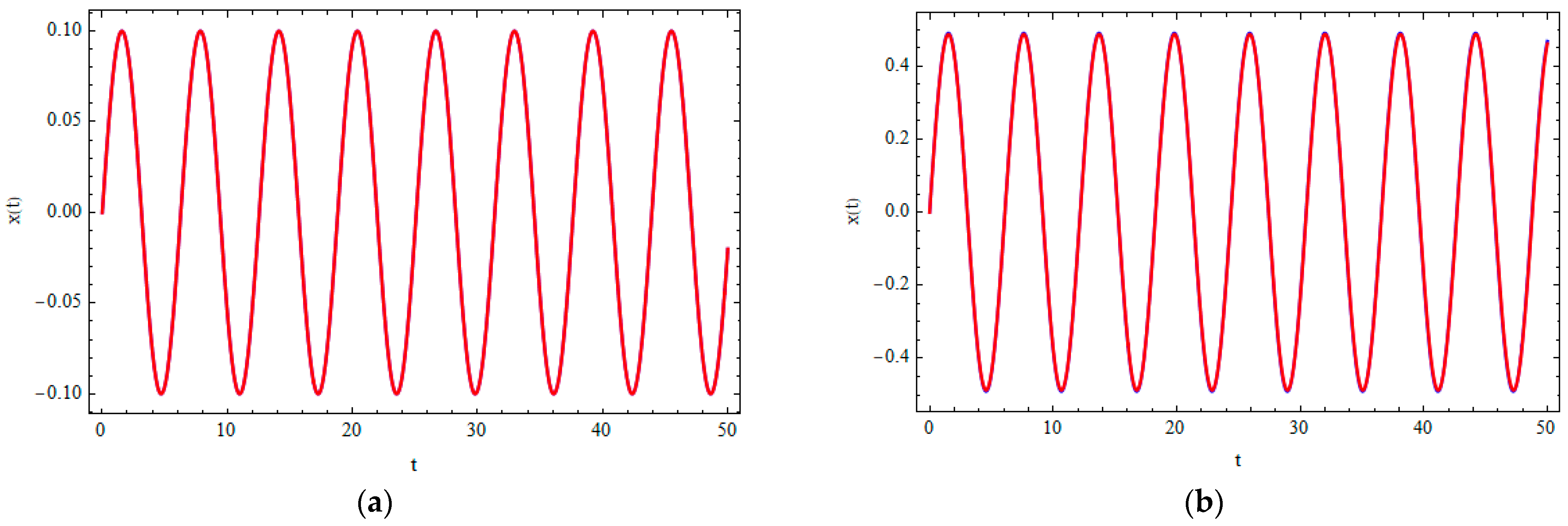
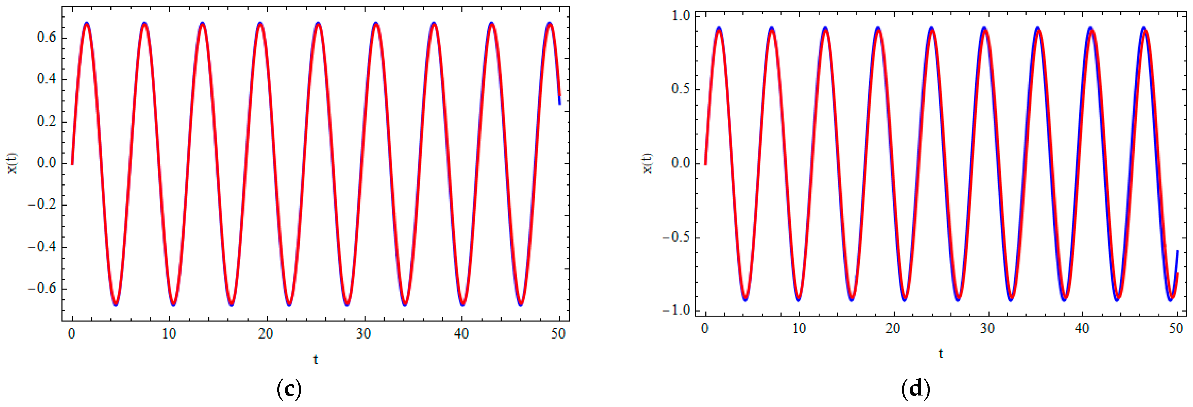
To assess the accuracy of the solutions obtained in cases 1 and 2, we compared the approximate analytical results derived using PEM with numerical solutions obtained via the fourth-order Runge–Kutta method. Figure 1 and Figure 2 illustrate these comparisons, corresponding to the present solutions (25) and (28), respectively.

3. Results and Discussion

The PEM was effectively applied to the nonlinear third-order Jerk equation, yielding accurate and consistent approximate analytical solutions. Two specific cases are explored: one involving displacement–velocity–acceleration interactions and another involving velocity coupled with acceleration-squared terms. The third-order approximations demonstrated strong agreement with numerical results obtained via the Runge–kutta method, as shown in Figure 1 and Figure 2, particularly for low to moderate oscillation amplitudes. Frequency–amplitude response curves indicated significant nonlinearity-induced shifts, showing both hardening and softening behavior depending on the nature of the Jerk function. The analytical expressions also successfully captured higher-order harmonic contributions—such as third and fifth harmonics—especially at larger amplitudes.

These findings highlight PEM’s effectiveness as a semi-analytical approach in solving the nonlinear Jerk-type. Unlike traditional perturbation methods, PEM does not depend on small parameters or linearization assumptions, making it well-suited for systems with strong nonlinearities. The method accurately models amplitude-dependent frequency behavior and provides deeper insights into the dynamics of nonlinear Jerk equations. The inclusion of higher-order harmonics reflects the impact of nonlinearity on waveform shape and energy distribution. Furthermore, PEM delivers closed-form solutions that support further theoretical investigations and sensitivity analyses. Overall, PEM proves to be a robust and flexible method in analyzing nonlinear oscillatory systems in areas such as applied mechanics, vibration analysis, and control engineering.

In contrast to perturbation methods that require small parameters or linearization, PEM directly incorporates nonlinear coupling terms, allowing it to capture amplitude-dependent frequency shifts and higher-harmonic contributions, while maintaining excellent agreement with numerical simulations. Figure 1 and Figure 2, therefore, serve not only as visual comparisons but also as demonstrations of PEM’s effectiveness, providing a compact analytical framework that accurately tracks nonlinear distortions in both frequency and waveform—an advantage over traditional perturbation approaches.

Figure 1: Shows comparison between the analytical solutions obtained using PEM (red line) and the numerical solution (blue line) for Equation (25). The numerical solution is generated using the classical fourth-order Runge–Kutta method to ensure stability and accuracy. The PEM solution closely follows the numerical response, reproducing the fundamental oscillation as well as nonlinear effects such as amplitude-dependent frequency shifts and higher-harmonic components.

Figure 2: Displays comparison between the analytical solutions obtained using PEM (red line) and the numerical solution (blue line) for Equation (28). The numerical solution is obtained using the fourth-order Runge–Kutta method under identical initial conditions and time-stepping parameters. The strong agreement highlights PEM’s ability to reproduce nonlinear distortions, including hardening/softening frequency shifts and waveform modifications arising from third- and fifth-order harmonics.

Taken together, Figure 1 and Figure 2 demonstrate PEM’s strength in handling strongly nonlinear Jerk equations. The method successfully models nonlinear frequency shifts—showing hardening or softening depending on the governing Jerk function—and naturally captures the emergence of higher harmonics that reshape the waveform at larger amplitudes. These features, often inaccessible to conventional perturbation methods, are clearly resolved within the PEM framework. The near-complete overlap with numerical simulations further confirms its robustness as a semi-analytical approach, making PEM a reliable tool in investigating nonlinear oscillators in applied mechanics and engineering contexts.

In addition,

Table 1. Displays a comparison between the exact and approximate values of the period for Equation (17).

$\mathit{A}$	${\mathbf{T}}_{\mathbf{e}}$	Current ${\mathbf{T}}_3$	RHBM [17]	HPM [13]	LPM [16]	HBM [22]	PEM [11]
0.1	6.275347	6.275350	6.275346837	6.27534684	6.275348	6.275346	6.275326
		(4.78 × 10−5)	(2.59 × 10−6)	(2.55 × 10−6)	(1.59 × 10−5)	(1.59 × 10−5)	(3.35 × 10−4)
0.2	6.252016	6.2520924	6.25201599	6.25201599	6.252028	6.252003	6.251690
		(0.001222)	(1.59 × 10−7)	(2.59 × 10−7)	(1.92 × 10−4)	(2.08 × 10−4)	(0.00521)
0.5	6.096061	6.09866	6.09606050	6.09605904	6.096491	6.095585	6.083668
		(0.042634)	(8.20 × 10−6)	(3.12 × 10−5)	(0.00706)	(0.00781)	(0.20329)
1	5.626007	5.653322	5.62599289	5.62579479	5.630343	5.619852	5.441398
		(0.485513)	(2.51 × 10−4)	(0.00377)	(0.07707)	(0.10940)	(3.28135)

and

Table 2. Shows a comparison between the exact and approximate values of the period for Equation (27).

$\mathit{A}$	${\mathbf{T}}_{\mathbf{e}}$	Current ${\mathbf{T}}_3$	RHBM [17]	HPM [13]	LPM [16]	HBM [22]
0.1	6.2753338	6.275338	6.2753338	6.27533378	6.275329	6.2753264
		0	0	0	(7.61 × 10−5)	(1.18 × 10−4)
0.2	6.251809	6.251887	6.25180911	6.25182078	6.251740	6.251690
		(0.001247)	(1.76 × 10−6)	(1.88 × 10−4)	(0.00110)	(0.00190)
0.5	6.088449	6.0914236	6.08848374	6.08815979	6.085649	6.083668
		(0.048856)	(5.71 × 10−4)	(0.00475)	(0.04599)	(0.07853)
1	5.527200	5.570066	5.52994105	5.50818960	5.477174	5.441398
		(0.775546)	(0.04959)	(0.343943)	(0.90509)	(1.55236)
1.5	4.690247	4.863291	4.72603111	4.44735707	4.412733	4.155936
		(3.689443)	(0.76295)	(5.17847)	(5.91683)	(11.39196)

provide quantitative evidence by comparing the third approximate period ${\mathrm{T}}_3$ obtained from the PEM with the exact values and other analytical methods. The deviations are remarkably small, for example, at amplitude 0.1, the PEM period is 6.275347 compared with the exact 6.275346837, an error of less than ${10}^{-6}$ Even at larger amplitudes, discrepancies remain minimal. Together with Figure 1 and Figure 2, these results provide both numerical and graphical validation of PEM’s accuracy and convergence, reinforcing the claim that PEM is a simple yet highly effective tool in capturing nonlinear frequency shifts and higher-harmonic behavior.

To validate the accuracy, we calculated the percentage error (%) according to its definition:

$$\mathrm{E}\mathrm{r}\mathrm{r}\mathrm{o}\mathrm{r}=\left|{\displaystyle \frac{{\mathrm{T}}_{\mathrm{e}\mathrm{x}\mathrm{a}\mathrm{c}\mathrm{t}}-{\mathrm{T}}_{\mathrm{A}\mathrm{p}\mathrm{p}}}{{\mathrm{T}}_{\mathrm{e}\mathrm{x}\mathrm{a}\mathrm{c}\mathrm{t}}}}\right|\times 100\%,$$

(30)

where various approximate periods obtained by ${\mathrm{T}}_{\mathrm{A}\mathrm{p}\mathrm{p}}$ and ${\mathrm{T}}_{\mathrm{e}\mathrm{x}\mathrm{a}\mathrm{c}\mathrm{t}}$ represent the corresponding exact period of the oscillator.

Finally, while earlier studies, such as Ismail and Yamani [21], employed hybrid schemes that combine PEM with Modified Iteration Methods to enhance convergence, the present work deliberately applies PEM in its pure form. This choice emphasizes PEM’s intrinsic ability to capture amplitude-dependent frequency shifts, higher-harmonic distortions, and nonlinear waveform modifications without auxiliary corrections. The results confirm that PEM alone provides a concise yet robust analytical framework, delivering accuracy comparable to more complex hybrid approaches while retaining greater simplicity and transparency. This highlights the dual contribution of the paper: establishing PEM as both a practical analytical tool for nonlinear Jerk equations and a benchmark framework against which hybrid or modified methods can be evaluated.

To assess the accuracy of the analytical approximations for the nonlinear Jerk Equations (17) and (27) against the corresponding reference solutions in Equations (25) and (28), three quantitative error indicators were utilized: the Root Mean Square Error (RMSE), the Relative RMSE, and the Maximum Absolute Error (Max Abs Error). The equations were first solved numerically using a high-order Runge–Kutta integration scheme to obtain the reference solution $x_{num}\left(t\right)$, while the analytical approximation $x_{approx}\left(t\right)$ was evaluated at the same discrete time points $t_i$. The RMSE, which quantifies the average deviation magnitude between the two solutions, was calculated as follows:

$$\mathrm{R}\mathrm{M}\mathrm{S}\mathrm{E}=\sqrt{{\displaystyle \frac{1}{N}}+{\sum }_{i=1}^N{\left[x_{num}\left(t_i\right)-x_{approx}\left(t_i\right)\right]}^2},$$

(31)

where N represents the total number of sampled points. To obtain a dimensionless and scale-independent indicator, the RMSE was normalized by the root-mean-square amplitude of the numerical solution, resulting in the Relative RMSE, which is defined as

$$\mathrm{R}\mathrm{e}\mathrm{l}\mathrm{a}\mathrm{t}\mathrm{i}\mathrm{v}\mathrm{e} \mathrm{R}\mathrm{M}\mathrm{S}\mathrm{E}={\displaystyle \frac{\mathrm{R}\mathrm{M}\mathrm{S}\mathrm{E}}{N\sqrt{\frac{1}{N}+\sum _{i=1}^N{\left[x_{num}\left(t_i\right)-x_{approx}\left(t_i\right)\right]}^2}}}.$$

(32)

Furthermore, the Maximum Absolute Error was determined as

$$\mathrm{M}\mathrm{a}\mathrm{x} \mathrm{A}\mathrm{b}\mathrm{s} \mathrm{E}\mathrm{r}\mathrm{r}\mathrm{o}\mathrm{r}=max\left|x_{num}\left(t_i\right)-x_{approx}\left(t_i\right)\right|,$$

(33)

to capture the largest pointwise deviation between the two solutions within the considered time interval. Collectively, these three metrics provide a comprehensive evaluation of both the overall and peak discrepancies, where lower values indicate stronger agreement and higher accuracy of the analytical approximation in reproducing the true system dynamics, as shown in

Table 3. Computes RMSE, Relative RMSE, and Maximum Absolute Error for Equation (17).

A	RMSE	Relative RMSE	Max Abs Error
0.1	0.0000220515	0.000311564	0.0000313245
0.5	0.0050616	0.0146871	0.0110108
1	0.0997455	0.1527548	0.2300944
1.5	0.4753127	0.5284609	1.0796243
2	1.1507117	1.0622366	2.5387488

and

Table 4. Computes RMSE, Relative RMSE, and Maximum Absolute Error for Equation (25).

A	RMSE	Relative RMSE	Max Abs Error
0.1	0.0000221	0.000312677	0.0000315208
0.5	0.0065785	0.0190583	0.0148713
1	0.178973	0.279584	0.4200002
1.5	0.98505	1.15267	2.15964
2	1.42245	1.48123	2.80166

.

To quantify the largest pointwise deviation between the two solutions over the considered time interval. Together, these three metrics offer a comprehensive assessment of both the overall and peak discrepancies, where smaller values signify closer agreement and higher accuracy of the analytical approximation in capturing the true system dynamics, as presented in Table 3 and Table 4.

Table 3 and Table 4 present a quantitative assessment of the PEM accuracy through the RMSE, Relative RMSE, and Maximum Absolute Error for the two nonlinear Jerk equations. The outcomes demonstrate that PEM maintains excellent consistency with the numerical (Runge–Kutta) results, particularly for small and moderate amplitudes where the errors remain below 10⁻³. As anticipated, the discrepancies increase with amplitude due to the intensification of nonlinear effects at larger oscillation levels. A comparative analysis reveals that the second case (Table 4) exhibits slightly higher errors than the first, suggesting that the velocity–acceleration-squared coupling produces stronger nonlinearity than the displacement–velocity–acceleration interaction. In general, the low RMSE and Maximum Absolute Error values confirm the robustness and convergence of PEM, while the gradual error increase at high amplitudes indicates that higher-order extensions or hybrid formulations—such as combining PEM with the Modified Iteration Method—could further enhance accuracy.

4. Conclusions

This paper introduced a straightforward and effective analytical technique, parameter expansion, to estimate the frequencies and periodic solutions of highly nonlinear oscillators described by a third-order nonlinear differential equation. The method’s key benefit lies in its simplicity, and the results it produced closely match numerical solutions, regardless of whether the oscillations have small or large amplitudes. In conclusion, this study successfully employed PEM to analyze complex dynamics of slender cantilever beams with flexible roots and intermediate lumped masses, systems governed by a highly nonlinear differential equation. The PEM provides a straightforward and accurate approximate analytical solution, demonstrating superior performance compared to other approximation techniques, particularly in physically realistic scenarios. By directly yielding analytical solutions while bypassing complex computations, PEM offers a quicker and more efficient approach in understanding and predicting the behavior of these challenging nonlinear oscillators, making it a valuable tool for engineering applications.

As a future study, coupled Jerk systems can be studied in multi-body mechanical constructions, interconnected electrical circuits, synchronized robotic arms, and physiological systems such as coupled neuromuscular reflexes. These systems frequently display complex behavior, including chaos, synchronization, bifurcations, and wave propagation, which are challenging to analyze using conventional linearization or perturbation techniques. PEM offers a systematic method for obtaining precise approximate solutions without limiting the research to minor parameters, facilitating a more profound understanding of stability, resonance, and control attributes. Utilizing PEM in coupled Jerk equations enables researchers to more accurately forecast system behavior across diverse conditions, optimize design parameters, and improve performance in both experimental and industrial contexts, thereby connecting theoretical nonlinear dynamics with practical engineering applications.