


Abstract
Detecting and identifying faults in industrial chemical plants is essential for safe and stable operation, and modern monitoring systems increasingly rely on deep learning to classify faults from multivariate sensor data. A practical obstacle to adoption is trust: most deep-learning diagnosers reach their decisions through a classification layer that operators cannot inspect, making it hard to see how the model maps process signals to a particular fault. This study targets fault diagnosis on the Tennessee Eastman (TE) process, a standard benchmark of simulated chemical-plant sensor data, and asks whether this final decision stage can be made directly inspectable without sacrificing accuracy. We propose CNN–Transformer–KAN (CTKAN), a hybrid model that learns local temporal patterns with a one-dimensional convolutional encoder, captures global inter-time-step dependencies with a Transformer encoder, and classifies faults with a Kolmogorov–Arnold Network (KAN) head whose learnable B-spline activations can be plotted and examined individually, in place of a conventional multi-layer perceptron (MLP). On the TE benchmark, CTKAN attains a Macro-F1 of 91.38 ± 0.26% over ten independent runs, comparable to a CNN + Transformer + MLP ablation (91.21 ± 0.32%) and a capacity-matched MLP-head variant (91.43 ± 0.37%) within seed-to-seed variability. The main finding is therefore not a higher score: at matched capacity the KAN and MLP heads are statistically indistinguishable in accuracy, so the KAN head’s value is to add a directly inspectable view of the classification stage at no measurable accuracy cost, helping process engineers sanity-check how the diagnoser separates faults in safety-critical settings.
1. Introduction
Industrial chemical processes such as petroleum refining, pharmaceutical manufacturing, and polymerization operate under complex, highly coupled conditions where equipment failures or process deviations can lead to catastrophic consequences including environmental contamination, economic losses, and threats to human safety [1,2]. In Industry 4.0 and smart manufacturing settings, data-driven process monitoring and fault diagnosis support predictive maintenance and safer plant operation [3,4,5,6,7,8]. The TE process, originally proposed by Downs and Vogel [9] as a realistic simulation of an industrial chemical plant, has become the most widely adopted benchmark for evaluating fault diagnosis algorithms. The TE process involves five major unit operations with 41 measured and 11 manipulated variables (52 in total); our experiments use 50 process variables after standard preprocessing, encompassing 20 distinct fault scenarios of varying difficulty that span step changes, random variations, slow drifts, and sticking valves.
Traditional fault diagnosis methods based on multivariate statistical analysis, such as principal component analysis (PCA) [10] and Partial Least Squares (PLS) [11], project high-dimensional process data into lower-dimensional subspaces and monitor statistical indices for anomaly detection. While these methods are mathematically well-founded and computationally efficient, they rely on linear assumptions that fundamentally limit their ability to capture the nonlinear dynamics inherent in complex chemical processes.
The advent of deep learning has provided powerful alternatives for nonlinear feature extraction from process monitoring data, with broad adoption across machine health monitoring pipelines [12]. One-dimensional convolutional neural networks (CNN1Ds) [13,14] apply local receptive fields to capture short-range temporal patterns such as transient spikes and sensor anomalies. However, standard CNN1Ds with small kernel sizes have limited receptive fields and cannot directly model long-range dependencies across distant time steps. Recurrent Neural Networks (RNNs), particularly Long Short-Term Memory (LSTM) networks [15], process sequential data step by step and can theoretically capture long-term dependencies, but in practice suffer from vanishing gradient problems and cannot be parallelized during training. Bidirectional variants have been applied to chemical-process fault diagnosis with improved performance [16]. The Transformer architecture [17], which employs self-attention mechanisms to directly compute pairwise relationships between all time steps, has shown promising results on TE fault diagnosis [18,19,20,21]. However, applying Transformers alone sacrifices the inductive bias for local pattern extraction that CNNs provide.
Several hybrid approaches have been explored. CNN-LSTM models combine local feature extraction with sequential modeling [22], while attention-based hybrids for process monitoring continue to evolve [20,21]. Kai et al. [23] benchmark MLP, CNN, LSTM, and Transformer models on multiple chemical-process benchmarks under varying temporal subsequence lengths. However, a fundamental limitation persists: their classification layers, typically multi-layer perceptrons (MLPs) with fixed activation functions, act as opaque decision boundaries that provide no insight into how extracted features map to fault categories. In safety-critical industrial applications, operators need not only accurate predictions but also explanations of the diagnostic reasoning [24,25]. When the decision behavior of the classification layer itself can be inspected, engineers and operators can verify how the diagnoser responds to individual process variables and audit the model before trusting its outputs in safety-critical operation, rather than relying on aggregate accuracy alone.
The recently proposed KAN [26] offers a promising direction for classification heads with directly plottable edge functions. Based on the Kolmogorov–Arnold representation theorem [27], KAN replaces fixed activation functions with learnable B-spline functions on network edges, enabling direct visualization of the learned nonlinear transformations. Recent applications of KAN to fault diagnosis in power Transformers [28] and rotating machinery [29] have demonstrated its potential. Preliminary studies have also explored KAN-based autoencoders for unsupervised fault detection on the TE process [30].
To address the dual challenges of multi-scale temporal feature extraction and limited classification-layer inspectability, this paper proposes CTKAN, a three-stage hybrid architecture. The central research question we investigate is whether a KAN-based classification head can provide useful, directly inspectable decision functions for industrial fault diagnosis without reducing classification accuracy compared with a conventional MLP head. CTKAN is organized into three stages:
Stage 1 (Local Feature Extraction): A CNN1D encoder with standard convolutions and a kernel size of three extracts local temporal features. With two CNN blocks (each containing two 1D convolutional layers), the receptive field covers approximately nine time steps, capturing short-range patterns while intentionally leaving global temporal structure for the subsequent stage.
Stage 2 (Global Dependency Modeling): A Transformer encoder with multi-head self-attention establishes dependencies across all time steps, complementing the CNN’s local view with global context.
Stage 3 (Inspectable Classification): A KAN classification head with two layers of learnable B-spline activation functions replaces the conventional MLP, enabling visualization of the nonlinear response curves learned during classification. Here, by inspectability, we mean that each learned activation function in the classification layer can be directly plotted and examined, as distinct from interpretability, i.e., explaining why a particular fault decision is made.
The main contributions of this work are summarized as follows:
- We propose CTKAN, a hybrid CNN–Transformer–KAN architecture that couples local temporal feature extraction (CNN) with global inter-time-step dependency modeling (Transformer) and a classification head whose per-edge B-spline activation functions can be plotted and inspected individually. The novelty lies in this inspectable-by-construction classification design rather than in maximizing benchmark accuracy.
- Under the reported TE protocol, CTKAN achieves a competitive Macro-F1 of 91.38 ± 0.26% over ten independent training runs among the four main-table architectures, and a factorial ablation quantifies the contribution of the Transformer stage.
- At matched parameter capacity (≈526k), the KAN and MLP classification heads yield comparable Macro-F1 (91.38 ± 0.26% vs. 91.43 ± 0.37%) within seed-to-seed variability; the distinguishing benefit of the KAN head is its directly inspectable B-spline activation curves rather than an accuracy gain.
- Through per-class analyses of hard-to-diagnose TE faults (IDV(3), IDV(9), IDV(15)), we document specific strengths and weaknesses of the model rather than presenting CTKAN as universally superior.
The remainder of this paper is organized as follows. Section 2 reviews related work on deep-learning fault diagnosis and positions CTKAN with respect to existing methods. Section 3 details the proposed CTKAN architecture and its training procedure. Section 4 describes the experimental setup and reports results on the TE benchmark, including ablation, inspectability, and sensitivity analyses. Section 5 discusses the main findings, parameter efficiency, and limitations, and Section 6 concludes the paper.
2. Related Work
This section reviews prior work relevant to the proposed CTKAN framework and positions our contribution. The discussion is organized along four dimensions that are central to inspectable fault diagnosis: (i) local temporal feature extraction, (ii) global temporal dependency modeling, (iii) the transparency of the classification layer, and (iv) evaluation on the TE benchmark. Section 2.1 reviews convolutional and recurrent approaches; Section 2.2 examines Transformer-based and hybrid models; Section 2.3 surveys KAN in fault diagnosis; Section 2.4 discusses the transparency of the classification layer; and Section 2.5 consolidates the comparison in a gap-analysis table and states the research gap that motivates CTKAN.
2.1. Convolutional and Recurrent Approaches
Data-driven fault diagnosis has evolved from classical multivariate statistical methods (such as principal component analysis and its dynamic variants [1,2,10,11]) toward deep-learning models that learn discriminative features directly from raw process data [12]. On the TE benchmark, this transition is well documented: Yin et al. [31] provided a widely used comparison of basic data-driven monitoring methods, and subsequent studies showed that deep models can surpass them; for example, the deep belief network of Zhang and Zhao [32] and the architecture comparison of Chadha and Schwung [33] both demonstrated that learned hierarchical features improve fault classification on TE.
Among deep architectures, convolutional neural networks (CNNs) exploit the local structure of multivariate time series through shared convolutional filters. Wu and Zhao [13] proposed a deep CNN for chemical-process fault diagnosis that learns discriminative features directly from raw signals, and Chen et al. [14] developed a one-dimensional convolutional autoencoder for unsupervised feature learning from multivariate processes. CNNs are computationally efficient and translation-invariant, but standard convolutions with small kernels have an inherently limited receptive field and therefore cannot directly capture dependencies that span distant time steps. Beyond architectural choices, the robustness of CNN-based diagnosers under changing operating conditions has been pursued through transfer learning: Siddique et al. [34] proposed a multistage transfer-learning framework that progressively adapts a pretrained convolutional network to sustain vibration-based fault discrimination across variable rotating-machinery speeds. Such strategies improve cross-condition generalization, but they retain a conventional classification head and target a sensing modality distinct from the multivariate chemical-process signals considered here.
RNNs, in particular LSTM networks [15], instead model temporal sequences through recurrent hidden states and can in principle represent long-range dependencies. Mou et al. [16] applied bidirectional RNNs to TE fault diagnosis and reported improved performance from bidirectional temporal modeling. However, recurrent models process sequences step by step, which precludes parallelization and leads to inefficient training, and they remain susceptible to vanishing-gradient effects on long sequences. Crucially, both CNN- and RNN-based diagnosers in this category retain a conventional MLP classification layer whose decision behavior cannot be inspected directly.
2.2. Transformer-Based and Hybrid Approaches
The Transformer architecture [17] replaces recurrence with self-attention, enabling each time step to attend to all others in parallel and thereby capturing global dependencies efficiently. This property has motivated a series of Transformer-based diagnosers for the TE process. Zhang et al. [18] proposed a generalized Transformer for TE fault diagnosis, and Labbaf-Khaniki et al. [19] introduced a twin Transformer with a gated dynamic learnable attention mechanism that achieved over 94% accuracy. More recent work has enriched the attention backbone with additional structure: Cao et al. [20] augmented a Transformer with a graph attention mechanism for complicated processes, and Zhang et al. [21] proposed a sequence-aware vision Transformer with feature fusion for complex industrial processes. Comparative studies have further mapped the design space: Lomov et al. [35] benchmarked a range of recurrent and convolutional temporal models, including LSTM, GRU, attention-augmented RNNs, and Transformers, on the extended TE dataset, and Kai et al. [23] systematically compared supervised deep-learning algorithms under different temporal subsequence lengths. In a recent deployment-oriented study, Khan et al. [36] combined physics-guided residuals with an attention-based convolutional–recurrent network (Conv1D–BiGRU) for early-warning fault detection on the TE process, coupling strong detection performance with probability calibration and SHAP-based feature attribution.
Hybrid designs combine complementary inductive biases. CNN–LSTM models, such as the optimized network of Chen et al. [22], cascade convolutional feature extraction with recurrent temporal modeling, inheriting both local sensitivity and sequential memory but also the training cost of recurrence. Across these Transformer-based and hybrid approaches, the emphasis is on maximizing predictive accuracy through more expressive encoders, while the classification layer remains a standard linear-plus-softmax head. Attention maps are sometimes presented as a form of explanation, but they describe where the encoder attends rather than how the final classification function transforms the pooled features, and they do not by themselves render the classification layer inspectable.
2.3. Kolmogorov–Arnold Networks in Fault Diagnosis
The Kolmogorov–Arnold representation theorem [27] states that any multivariate continuous function can be expressed as a finite superposition of continuous univariate functions and addition. KAN [26] operationalizes this result by replacing the fixed node activations of an MLP with learnable univariate functions, parameterized as B-splines, placed on the network edges. A direct consequence is that every learned edge function can be plotted and examined, which gives KAN an intrinsic, structural form of transparency at the level of individual connections.
KAN has been adopted across several fault-diagnosis domains. Cabral et al. [28] applied KAN to fault diagnosis of oil-immersed power Transformers; Rigas et al. [29] used KAN for explainable fault classification and severity diagnosis in rotating machinery; Wang et al. [37] combined KAN with hypergraph message passing for rolling-bearing diagnosis in noisy environments; and Morales et al. [30] explored KAN-based autoencoders for unsupervised anomaly detection on the TE process. Livieris [38] showed that integrating convolutional layers with KAN (C-KAN) improves time-series forecasting accuracy, providing evidence that KAN can be productively combined with convolutional front ends. These studies employ KAN for a variety of purposes (improving predictive accuracy [28,37], time-series forecasting [38], unsupervised anomaly detection [30], or explainable severity estimation [29]), but in nearly all of them, KAN serves as the principal predictor, and its functional transparency, when noted at all, is incidental rather than the explicit object of evaluation. Moreover, the KAN is typically used either as a standalone classifier or in combination with a single feature extractor; except for the unsupervised autoencoder of [30], it is rarely deployed as an inspectable classification head on top of a model that jointly captures local and global temporal structure for supervised TE fault classification. In contrast, the present work uses the KAN head specifically as an inspectable classification layer and evaluates whether it can deliver this additional qualitative inspection capability while maintaining predictive performance comparable to a conventional MLP head, a question of head-level inspectability, decoupled from raw accuracy, that prior KAN fault-diagnosis studies have not addressed.
2.4. Transparency of the Classification Layer
Because deep diagnosers are typically opaque, a substantial body of work applies post hoc explainable-AI (XAI) techniques to interpret them. Jang et al. [24] applied explainable AI to fault diagnosis of industrial processes, and Cacao et al. [25] surveyed XAI methods for industrial fault diagnosis; more recently, Khan et al. [36] paired an attention-based CRNN on the TE process with SHAP-guided feature selection and probability calibration to produce operator-facing explanations. Such techniques (for example, SHAP and gradient-based attributions) operate after training on an unchanged, opaque model and produce approximate importance scores for inputs or features. They are valuable but indirect: the classification layer itself remains a black box, and the explanation is an external estimate rather than a property of the model. This motivates a complementary direction, namely making the classification layer structurally inspectable by construction, the role played by the KAN head in the present work, whose learned per-edge activation functions can be plotted directly without any post hoc attribution.
2.5. Comparative Analysis and Research Gap
Table 1 consolidates the preceding discussion along the four dimensions introduced above.
Table 1.
Comparative analysis of representative fault-diagnosis approaches across four key dimensions; the last column summarizes the main gap of each approach.
As the table makes explicit, existing approaches each leave at least one dimension unaddressed: CNNs capture local structure but not long-range dependencies; RNNs model sequences but are difficult to train and remain opaque; Transformer-based and hybrid models achieve strong accuracy yet retain opaque classification heads; and KAN-based methods provide an inspectable functional form but have not been integrated with a combined CNN–Transformer encoder for supervised TE fault classification. In short, no prior method simultaneously (i) extracts local features with a CNN, (ii) models global temporal dependencies with a Transformer, and (iii) classifies through an inspectable KAN head, while being evaluated on the standard TE benchmark.
CTKAN is designed to fill precisely this gap. It assigns local and global temporal modeling to a CNN encoder and a Transformer encoder with deliberately complementary, non-overlapping roles, and it replaces the conventional MLP classification head with a KAN head whose B-spline edge activations can be inspected directly. Consistent with our central claim, the contribution of the KAN head is classification-layer inspectability rather than a peak-accuracy gain: as reported in Section 4.3 and Section 4.4, CTKAN attains accuracy comparable to a capacity-matched MLP-head counterpart while additionally providing a directly plottable view of the learned classification-layer transformations.
3. Proposed Method
This section presents the proposed CTKAN framework in detail. We first formalize the fault-diagnosis task (Section 3.1) and outline the overall architecture (Section 3.2). We then describe the three stages in turn—the CNN encoder for local feature extraction (Section 3.3), the Transformer encoder for global dependency modeling (Section 3.4), and the KAN classification head (Section 3.5)—before presenting the training procedure (Section 3.6) and summarizing the complete method as pseudocode (Section 3.7).
3.1. Problem Formulation
Industrial process fault diagnosis is formulated as a supervised multivariate time-series classification problem. A monitored process is characterized by D sensors and manipulated variables sampled over time, and a single diagnostic decision is made on a fixed-length temporal window. Formally, one sample is
where T is the number of time steps contained in the window and xt is the vector of D process variables observed at time step t. In this study, T = 20 and D = 50. Each window is associated with an operating-condition label
where y = 0 denotes the normal operating condition and y = 1, …, 20 denote the twenty fault types of the Tennessee Eastman benchmark, giving C = 21 classes in total. Because the process variables differ in physical units and dynamic range, every variable is standardized with the per-variable mean and standard deviation estimated on the training set only; these statistics are then reused unchanged for validation, testing, and online inference:
where μd and σd are the training-set mean and standard deviation of the d-th variable, and x̃t,d is the standardized value. The objective is to learn a parametric mapping fθ that converts a standardized window X̃ into a posterior distribution over the C classes,
where pc is the predicted posterior probability of class c and θ collects all trainable parameters. The predicted operating condition is obtained by maximum a posteriori selection:
X = [x1, x2, …, xT]⊤ ∈ ℝT×D, xt ∈ ℝD
y ∈ Y = {0, 1, …, C − 1}, C = 21
x̃t,d = (xt,d − μd)/σd, d = 1, …, D
p = fθ(X̃) ∈ [0, 1]C, Σc=1C pc = 1
ŷ = argmaxc ∈ {1,…,C} pc
The parameters θ are estimated by minimizing the empirical cross-entropy risk defined in Section 3.6 (Equation (25)).
Beyond this formulation, it is useful to state explicitly the evaluation objectives that the proposed design is intended to satisfy and that the experiments in Section 4 are constructed to test. We organize them as three research questions. (O1) Architectural contribution: How much does the global-dependency-modeling Transformer stage contribute beyond the local features extracted by the CNN encoder? This motivates the factorial ablation in Section 4.3. (O2) Head-level inspectability versus accuracy: Can the KAN classification head, at matched parameter capacity, maintain predictive performance comparable to a conventional MLP head while additionally exposing directly inspectable activation functions? This is the central hypothesis of the paper and motivates both the capacity-matched comparison (Section 4.3) and the inspectability analysis (Section 4.4). (O3) Robustness: How sensitive is the model to its principal hyperparameters, and does training converge under the reported protocol? This motivates the sensitivity and convergence study in Section 4.6. Stating these objectives here links the architectural choices detailed in the following subsections to the specific experimental analyses reported later.
3.2. Overall Architecture
As illustrated in Figure 1, the proposed CTKAN realizes the mapping fθ as a composition of three sequential stages with complementary roles: a CNN encoder that extracts local temporal features, a Transformer encoder that models global temporal dependencies, and a KAN head that performs inspectable classification. Let d denote the shared hidden dimension (d = 128). In the first stage, the standardized window is mapped to a sequence of local feature vectors,
Hc = Ecnn(X̃; θcnn) ∈ ℝT×d
Figure 1.
Overall architecture of the proposed CTKAN model. The input multivariate time series passes through three stages: a CNN encoder for local feature extraction, a Transformer encoder for global dependency modeling, and a KAN head for inspectable classification. The circled numbers ①–③ denote the three sequential stages of CTKAN (Stage 1: CNN encoder for local feature extraction; Stage 2: Transformer encoder for global dependency modeling; Stage 3: KAN head for inspectable classification). The different background colors are used only to visually distinguish the functional modules (input/output, CNN encoder, Transformer encoder, pooling, and KAN head) and carry no additional meaning.
In the second stage, the local features are contextualized by global self-attention while preserving the sequence length,
Ht = Etrans(Hc; θtrans) ∈ ℝT×d
The contextualized sequence Ht = [h1, …, hT], with ht ∈ ℝd its t-th time-step row, is then collapsed into a single window-level descriptor by temporal mean pooling followed by layer normalization,
z = LayerNorm ((1/T) Σt=1T ht) ∈ ℝd
Finally, the descriptor is mapped to class posteriors by the two-layer KAN head followed by a softmax,
so that the full model is the composition fθ = softmax ∘ gkan ∘ (LayerNorm ∘ Pool) ∘ Etrans ∘ Ecnn with θ = {θcnn, θtrans, θkan}. The three stages are detailed in Section 3.3, Section 3.4 and Section 3.5, the end-to-end training procedure in Section 3.6, and the complete offline training and online inference workflow is summarized as Algorithm 1 in Section 3.7.
p = softmax (gkan(z; θkan)) ∈ ℝC
3.3. CNN Encoder for Local Feature Extraction
The CNN encoder transforms the raw standardized variables into local temporal feature representations through a stack of L one-dimensional convolutional blocks (L = 2). Treating the standardized window as a multi-channel temporal signal U(0) = X̃⊤ ∈ ℝD×T, each block applies two convolution–batch-normalization–ReLU operations together with a residual shortcut. For the l-th block, the two convolutional layers are
and the block output combines the second convolution with a residual connection,
where ∗ denotes one-dimensional convolution with kernel size k = 3 and symmetric (non-causal) padding that preserves the sequence length; W and b are learnable kernels and biases; BN is batch normalization; and S(l) is the identity when the input and output channel counts match and a 1 × 1 convolution otherwise. All blocks use d = 128 output channels, and the encoder output is Hc = (u(L))⊤ ∈ ℝT×d. With L = 2 blocks and kernel size k, the effective receptive field is
which equals nine time steps for L = 2 and k = 3. This receptive field is deliberately kept smaller than the window length T = 20, so that the CNN encoder captures short-range local patterns while leaving the modeling of longer-range temporal dependencies to the subsequent Transformer encoder. The sensitivity of the diagnosis performance to the kernel size k is analyzed in Section 4.6.
a(l) = ReLU (BN (W1(L) ∗ u(l−1) + b1(L)))
u(l) = ReLU (BN (W2(L) ∗ a(l) + b2(L)) + S(l) (u(l−1)))
RF = 1 + 2 · L · (k − 1)
3.4. Transformer Encoder for Global Dependency Modeling
The Transformer encoder [17] models global temporal dependencies among the local features produced by the CNN stage. Because self-attention is permutation-invariant, sinusoidal positional encodings are first added to inject temporal order:
where t indexes the time step and i indexes the feature dimension. Each of the N = 2 encoder layers is composed of a multi-head self-attention (MHSA) sublayer and a position-wise feed-forward (FFN) sublayer, each wrapped by a residual connection and layer normalization. For head j, the queries, keys, and values are linear projections of the layer input Z,
and the scaled dot-product attention for that head is
where dk = d/h is the per-head dimension and h = 8 is the number of heads. The head outputs are concatenated and linearly projected,
PE(t,2i) = sin(t/10,0002i/d), PE(t,2i+1) = cos(t/10,0002i/d)
Z(0) = Hc + PE
Q(j) = Z WQ(j), K(j) = Z WK(j), V(j) = Z WV(j)
head(j) = softmax(Q(j) (K(j))⊤/√(dk)) V(j)
MHSA(Z) = Concat (head(1), …, head(h)) WO
The attention sublayer output is then formed with a residual connection and layer normalization,
followed by the position-wise feed-forward sublayer with inner dimension dff = 256 and a GELU nonlinearity,
Z′ = LayerNorm (Z + MHSA(Z))
FFN(Z′) = GELU (Z′ W1 + b1) W2 + b2
Z″ = LayerNorm (Z′ + FFN(Z′))
Stacking N = 2 such layers and applying a final layer normalization yields the contextualized sequence Ht used in Equation (7).
3.5. KAN Classification Head
Unlike a conventional MLP head, in which each neuron applies a fixed nonlinearity to a learned linear combination of its inputs, the KAN [26] head places a learnable univariate activation function on every edge. Each such edge function is parameterized as the sum of a SiLU base term and a B-spline expansion,
where wb is a learnable scalar weight, SiLU is the sigmoid-weighted linear unit, ci are learnable spline coefficients, Bi are B-spline basis functions of order s = 3 defined on a uniform grid of size G (G = 5 by default), and the SiLU activation is
φ(x) = wb · SiLU(x) + Σi=1G+s ci Bi(x)
SiLU(x) = x · σ(x), σ(x) = 1/(1 + e−x)
A KAN layer that maps an n-dimensional input u to an m-dimensional output sums the edge functions over the input coordinates,
where φq,p is the learnable activation on the edge connecting input p to output q. The classification head stacks two such layers,
and the logits o are converted to posteriors by the softmax of Equation (9). Because every edge activation φq,p is an explicit univariate function, it can be directly plotted and examined after training; this is the inspectability property analyzed in Section 4.4. The influence of the grid size G on both accuracy and the smoothness of the learned activations is studied in Section 4.6.
(Φ(u))q = Σp=1n φq,p (up), q = 1, …, m
h = Φ1(z) ∈ ℝ64, o = Φ2(h) ∈ ℝC
3.6. Training Procedure
The entire CTKAN model is trained end-to-end by minimizing the multi-class cross-entropy loss over the training set,
where N is the number of training windows, yn is the one-hot encoding of the label of window n, and pn is the corresponding predicted posterior. Optimization uses the Adam optimizer [39] with an initial learning rate of 1 × 10⁻³, weight decay 1 × 10⁻⁴, batch size 128, and a budget of 100 epochs. The learning rate follows a cosine-annealing schedule [40],
where e is the current epoch, E = 100 is the total number of epochs, and ηmax and ηmin are the initial and final learning rates. Gradient norms are clipped to 1.0 for stability. After every epoch, the model is evaluated on the validation set, and the checkpoint achieving the highest validation Macro-F1 is retained as the final model. The convergence behavior of this schedule over the 100-epoch budget is reported in Section 4.6.
L = −(1/N) Σn=1N Σc=1C yn,c log pn,c
ηe = ηmin + (1/2)(ηmax − ηmin) (1 + cos(e π/E))
3.7. Overall Algorithm
Figure 2 depicts the overall workflow of the proposed CTKAN-based fault diagnosis framework, and Algorithm 1 formalizes the complete pipeline, covering both the offline training stage and the online inference stage. The offline stage estimates the normalization statistics, trains the three-stage network, and selects the best checkpoint, whereas the online stage standardizes each newly acquired process window with the stored statistics, performs inference, and optionally exposes the KAN edge activations for classification-layer auditing before a fault decision is reported.
| Algorithm 1. Offline training and online inference of CTKAN |
| Input: training set Dtr, validation set Dval; epochs E; batch size B; learning-rate bounds (ηmax, ηmin). Output: trained parameters θ* of the CTKAN model. Offline training stage: 1: Compute per-variable mean μ and standard deviation σ on Dtr 2: Standardize all windows in Dtr and Dval using Equation (3) 3: Initialize parameters θ = {θcnn, θtrans, θkan} 4: for e = 1 to E do 5: for each mini-batch (X, y) in Dtr do 6: Hc ← CNN-Encoder(X) // Equations (10)–(12) 7: Ht ← Transformer-Encoder(Hc) // Equations (13)–(20) 8: z ← LayerNorm(MeanPool(Ht)) // Equation (8) 9: p ← softmax(KAN-Head(z)) // Equations (9) and (21)–(24) 10: L ← CrossEntropy(p, y) // Equation (25) 11: Update θ with Adam using the gradient of L 12: end for 13: Update the learning rate by cosine annealing // Equation (26) 14: Evaluate Macro-F1 on Dval; keep the best θ* so far 15: end for 16: return θ* Online inference stage: 17: Acquire a new process window Xnew and standardize it with stored μ, σ // Equation (3) 18: p ← fθ*(Xnew) // Equations (6)–(9) 19: ŷ ← argmaxc pc // Equation (5) 20: (optional) Plot the KAN edge activations φ for classification-layer auditing // Equation (21) 21: return predicted fault ŷ and inspection plots |
Figure 2.
Overall workflow of the proposed CTKAN-based fault diagnosis framework. In the offline stage, historical Tennessee Eastman data are standardized with training-set statistics, segmented into fixed-length windows, and used to train the three-stage CTKAN model, from which the checkpoint with the best validation Macro-F1 is retained. In the online stage, each newly acquired process window is standardized with the stored statistics and classified by the trained model; the learned KAN edge activations can additionally be inspected for classification-layer auditing before a fault decision is reported. The blue and green backgrounds distinguish the offline training and online inference stages, respectively. The orange dashed arrow indicates deployment of the trained model to the online stage, and the red dashed arrow indicates optional feedback for retraining or fine-tuning with newly labelled data.
4. Experiments and Results
This section reports the empirical evaluation of CTKAN on the Tennessee Eastman benchmark. Section 4.1 describes the experimental setup, including the dataset, preprocessing, baselines, and implementation details. Section 4.2 presents the main comparison results, Section 4.3 the ablation study, and Section 4.4 the inspectability analysis. Section 4.5 examines hard-to-diagnose faults, and Section 4.6 reports the hyperparameter-sensitivity and convergence analyses.
4.1. Experimental Details
This subsection consolidates the experimental setting: the datasets and their splits (Section 4.1.1), the baselines and CTKAN configuration (Section 4.1.2), and the 2 × 2 factorial ablation design (Section 4.1.3). The training procedure and reproducibility practices (optimizer, schedule, epochs, reproducibility settings, hardware, and metrics) are described in Section 3.6.
4.1.1. Datasets
Table 2 summarizes the TE benchmark. The TE benchmark [9] simulates a plant-wide chemical process; its 21 operating conditions (one normal + 20 fault scenarios) are recorded over 50 process variables (selected from the 41 measured and 11 manipulated TE variables) with 20 time steps per sample, totaling about 163,400 samples split into 104,500 training, 26,200 validation, and 32,700 test samples using the official train/test partition and a grouped stratified train-only validation split with z-score normalization computed exclusively from training data.
Table 2.
Summary of the TE benchmark used in this study.
4.1.2. Baselines
Table 3 lists the four end-to-end configurations compared in this study. CNN1D reuses CTKAN’s CNN encoder with an MLP head; RNN is a two-layer bidirectional LSTM; the standalone Transformer operates at = 64; CTKAN combines the CNN encoder (hidden dimension 128) with a Transformer encoder and the two-layer KAN head (head hidden 64). Each model follows its own standard configuration rather than a single matched-capacity setting, so Table 3 above compares end-to-end architectures as typically deployed.
Table 3.
Configurations of the four end-to-end models compared in this study.
4.1.3. Ablation Design
To isolate the contributions of the Transformer encoder and the KAN head, we adopt a 2 × 2 factorial ablation: the CNN encoder is always present, while the Transformer stage and the KAN head are each toggled independently. The CNN + Transformer + MLP configuration (denoted “CNN + Trans. + MLP”) directly represents a CNN–Transformer architecture with an MLP classification head, serving as an implicit CNN–Transformer baseline within the ablation design without requiring a separately trained fifth model. This factorial design lets us read the Transformer contribution and the KAN head contribution from the same four cells, rather than from two independent comparisons.
4.2. Main Comparison Results on the TE Dataset
As shown in Table 4 and Figure 3, the four main-table architectures are directly comparable on Macro-F1 with error bars; CTKAN attains competitive Macro-F1 with comparatively small variability among the four. The standalone CNN1D and RNN (BiLSTM) baselines obtain 90.23 ± 0.47% and 89.75 ± 0.42%, respectively, while the Transformer reaches 91.28 ± 0.26% on a substantially smaller parameter budget (72k vs. CNN1D’s 194k). Stacking a Transformer encoder on the CNN and switching to the inspectable KAN head (CTKAN) yields 91.38 ± 0.26%. Table 5 shows that the CNN + Transformer + MLP cell reaches 91.21 ± 0.32%, slightly below CTKAN; the differences among the top three configurations are within seed-to-seed variability over ten runs, so we present CTKAN as a competitive option whose distinguishing feature is classification-layer inspectability rather than as the strongest accuracy configuration. Parameter asymmetry between the MLP and KAN heads is addressed in Section 5.2 with a capacity-matched ablation.
Table 4.
Comparison of fault diagnosis methods on the TE benchmark (100 epochs). Bold entries denote the proposed CTKAN model.
Figure 3.
TE Macro-F1 of the four main-table architectures (mean ± std over ten independent training runs). Error bars show the standard deviation across seeds.
Table 5.
Ablation study on the TE benchmark (100 epochs).✓and✗indicate inclusion and exclusion of the Transformer stage and KAN head, respectively. Bold entries denote the proposed CTKAN configuration.
4.3. Ablation Study
Figure 4 visualizes the same ablation, highlighting that the CNN + Transformer configurations cluster slightly above the CNN-only configurations on Macro-F1.
Figure 4.
Factorial ablation of Macro-F1 on TE (mean ± std over ten independent training runs). CTKAN is competitive with the CNN + Transformer + MLP configuration; differences are within seed-to-seed variability.
Effect of the Transformer: Models without Transformer (avg F1 ≈ 90.36%) vs. with Transformer (avg F1 ≈ 91.30%) show ~0.94% (about one percentage point) consistent improvement, confirming global attention provides valuable context beyond the CNN’s local receptive field.
Effect of the KAN head: After ten-seed training, the KAN head edges the MLP head in both pairings (without Transformer: 90.48 ± 0.38% vs. 90.23 ± 0.47%; with Transformer: 91.38 ± 0.26% vs. 91.21 ± 0.32%), but in both cases the gap is well within seed-to-seed variability and should be read as comparable performance rather than a clear KAN advantage. The KAN head’s distinguishing benefit on this benchmark is its inherent inspectability through directly plottable B-spline activation curves.
Capacity-matched ablation. Because the CNN + Trans. + KAN configuration (526,101 parameters) and the CNN + Trans. + MLP configuration (459,413 parameters) differ in parameter count, we additionally trained a capacity-matched MLP-head variant (CNN + Trans. + MLP, matched, 526,613 parameters) with the same ten seeds. It reaches 91.43 ± 0.37% Macro-F1, comparable to CTKAN (91.38 ± 0.26%) within seed-to-seed variability. At equal capacity, the MLP head and the KAN head therefore yield comparable Macro-F1 on the TE protocol within seed-to-seed variability; the KAN head’s contribution remains the directly inspectable B-spline activations rather than an accuracy gain.
4.4. Inspectability Analysis
A key motivation for incorporating KAN is classification-layer inspectability. We present three complementary visualization analyses using a representative TE checkpoint. All three analyses operate on learned internal representations rather than raw sensor variables; CTKAN additionally applies post-pooling LayerNorm before feature extraction for t-SNE, which is not used for the other three models.
4.4.1. Feature Space Visualization via t-SNE
Figure 5 shows t-SNE [41] visualizations of the learned feature representations from all four models on the TE test set. Silhouette scores computed on PCA-reduced features do not rank CTKAN first in this checkpoint: CNN1D obtains 0.377, RNN 0.371, Transformer 0.423, and CTKAN 0.271. Therefore, this figure is used as a diagnostic visualization rather than proof that CTKAN has the clearest global feature separation. Note: CTKAN features are extracted after an additional post-pooling LayerNorm that is not applied to the other three models, which may partially account for the observed silhouette difference and means this comparison is not strictly apples-to-apples.
Figure 5.
t-SNE visualization of the learned penultimate-layer feature representations of the four main models, namely CNN1D, RNN (BiLSTM), Transformer, and CTKAN, on the TE clean test set (120 stratified samples per class; each point is one window, colored by its TE class label, with 0 denoting the normal condition and 1–20 the fault types). The projection is qualitative support rather than primary evidence of CTKAN superiority; the per-model silhouette scores and their interpretation are discussed in the text above.
To verify that the small Macro-F1 differences reported above are not artifacts of seed selection, we performed paired significance tests on the ten-seed Macro-F1 distributions, taking CTKAN as the reference. For each competing model, we report the paired t-test p-value, the Wilcoxon signed-rank p-value, and the 95% confidence interval of the paired difference (CTKAN minus the competitor, in percentage points). The results are summarized in Table 6.
Table 6.
Paired significance tests of Macro-F1 against CTKAN over ten independent training runs. ΔMacro-F1 (pp) is the mean paired difference (CTKAN minus competitor) in percentage points; the 95% CI refers to that difference; p-values are from the paired t-test and the Wilcoxon signed-rank test.
Two conclusions follow. First, CTKAN significantly outperforms the CNN1D and RNN baselines and the CNN + KAN configuration without the Transformer stage (all p < 0.001 under both tests), confirming that the Transformer encoder contributes a real improvement rather than seed-level noise. Second, and central to this paper, CTKAN, the standalone Transformer, the CNN + Transformer + MLP ablation, and the capacity-matched MLP head are statistically indistinguishable on Macro-F1 (all p > 0.05 under both tests). In particular, at matched parameter capacity, the KAN and MLP heads differ by only −0.05 pp with a 95% confidence interval of [−0.45, 0.35] pp that comfortably contains zero (paired t-test p = 0.79). This provides direct statistical support for our central claim: the KAN head is not introduced for accuracy gains (at equal capacity, it performs on par with an MLP head), but for the classification-layer inspectability defined in Section 3.4.
4.4.2. Attention Weight Analysis
Figure 6a,b present attention weights from CTKAN’s Transformer (final layer, averaged across heads). The global attention matrix shows approximately uniform attention (expected for T = 20), with subtle temporal biases. Class-averaged vectors reveal fault-specific temporal weighting patterns.
Figure 6.
(a) Global mean self-attention matrix from CTKAN’s final Transformer layer. Note: attention values span a narrow range (≈0.048–0.052), within ±4% of the uniform baseline 1/T = 0.050; the colormap is auto-scaled to this range, so visual contrast does not reflect large absolute differences between time steps. (b) Per-class attention vectors showing fault-specific temporal attention patterns. Note: as in Figure 6a, all values lie within ±4% of 1/T = 0.050; patterns should be interpreted as relative tendencies rather than strong temporal selection.
4.4.3. KAN Activation Curve Visualization
Figure 7a,b display the learned B-spline activation functions from the first KAN layer. The response norm plot (7a) shows diversity in learned transformations across 128 input channels. The top 10 most nonlinear channels (7b) exhibit complex S-shaped or peaked responses, while linear channels contribute through simple scaling. This visualization provides classification-layer inspectability unavailable with standard MLP heads. Among the top nonlinear channels in Figure 7b, several indices recur across the reported checkpoint, indicating that the KAN head allocates stronger spline-shaped transformations to a subset of latent dimensions rather than applying a uniform linear map. Unlike an MLP head, whose weight matrices require post hoc attribution to interpret, each KAN edge function can be plotted directly, allowing operators to check whether a latent dimension is saturated, inactive, or threshold-like before classification; this is a qualitative diagnostic view on learned features rather than a claim of higher accuracy. Because these curves operate on pooled latent dimensions rather than on raw sensors, we additionally provide a preliminary Integrated-Gradients attribution that traces the most inspectable latent channels back to the underlying TE process variables (Section 4.7); for each such channel the attribution concentrates on a small group of variables, giving an engineer a concrete, if preliminary, link from an inspectable activation curve to the physical measurements that drive it.
Figure 7.
(a) KAN layer 1 L2 response norm per input channel. Each colored line corresponds to one latent input channel of KAN layer 1; line color indicates the channel index (colorbar).Channels with steeper curves indicate stronger learned nonlinearities. Note: all curves converge near x = 0 because the B-spline basis functions have compact support and taper to zero at the grid boundary; this is a boundary artifact of the spline parameterization, not an indication that the learned functions are zero at x = 0. (b) Top 10 most nonlinear KAN channels (indices: 26, 113, 25, 55, 29, 119, 44, 38, 109, 12). NL ratio (residual after best-fit linear subtraction, normalized by signal norm) quantifies deviation from linearity; values near 0 indicate near-linear response. Edge functions are extracted directly from model weights to avoid B-spline boundary contamination.
4.5. Analysis of Hard-to-Diagnose Faults
Table 7 reports per-class F1 for three TE fault conditions known to be challenging across all six architectures. Fault 3 (IDV(3), step change in D feed temperature) is well handled by Transformer-based models: CTKAN (94.2 ± 1.0%), Transformer (94.0 ± 0.9%), and CNN + Trans. + MLP (93.6 ± 1.0%) cluster within roughly one percentage point of each other and are about 2.6 percentage points ahead of CNN1D (91.6 ± 0.7%). Fault 9 (IDV(9), random variation in D feed temperature) is moderately difficult: CTKAN (82.5 ± 1.1%) attains the highest mean among the six, slightly above the standalone Transformer (81.4 ± 1.5%) and CNN + Trans. + MLP (81.0 ± 1.0%). Fault 15 (IDV(15), sticking valve in condenser cooling water) remains the most challenging condition across all models, with F1 ranging from 28.4% (CNN1D) to 46.1% (Transformer). Notably, the standalone Transformer (46.1 ± 1.8%) outperforms CTKAN (39.4 ± 4.0%) on Fault 15, suggesting that pure global attention can be more effective than the hybrid architecture for this fault type. These per-class differences underscore that aggregate Macro-F1 alone does not capture the full picture; model selection for safety-critical deployments should consider class-specific performance on the target fault catalog. Figure 8 plots the same per-class F1 values, making the model-specific differences on Fault 15 visually salient. Figure 9 places the CTKAN class-averaged attention maps for these three faults side by side; the per-class temporal patterns are subtle and should be read as relative tendencies, consistent with the narrow attention range noted for Figure 6a.
Table 7.
Per-class F1 (%, mean ± std) for hard-to-diagnose fault conditions on the TE benchmark. Class k corresponds to fault IDV(k). Best result per row is bold.
Figure 8.
Per-class F1 on hard-to-diagnose TE faults (Fault 3, 9, 15) across six architectures (mean ± std). Aggregate Macro-F1 alone does not capture model-specific behavior on individual faults.
Figure 9.
Class-averaged self-attention maps for Faults 3, 9, and 15 from a representative CTKAN checkpoint. Maps are diagnostic visualizations of learned temporal weighting; they should be interpreted as relative tendencies rather than absolute selection.
To move beyond aggregate scores, we examined the dominant misclassification targets for these faults, aggregated over all ten test runs. Fault 3 is cleanly separated (96.0% recall, 92.5% precision), its only notable leakage being 3.3% of windows assigned to Fault 9. Fault 9 is harder (77.8% recall, 87.7% precision) and spreads across several neighbors, namely Fault 3 (7.3%), Fault 16 (7.1%), Fault 15 (3.7%) and Normal (3.6%), rather than failing on a single competitor. The behavior of Fault 15 is the most informative: 47.2% of its windows are predicted as Fault 16 and a further 11.0% as Normal, leaving only 36.1% correctly recalled. The confusion is bidirectional: Fault 16 is in turn predicted as Fault 15 in 29.4% of its windows and as Normal in 8.4%, so Faults 15 and 16 form a mutually entangled pair that all six architectures, including CTKAN, resolve only partially. This pattern points to a data-level rather than a model-level cause: IDV(15) (a sticking condenser cooling-water valve) and IDV(16) (an unknown disturbance) produce low-amplitude, overlapping signatures whose inter-class separation within a 20-step window is small, and both also drift toward the Normal operating region. Consistent with this interpretation, the same hard faults remain difficult across every architecture in our study and across the TE benchmark literature reviewed in Section 2, indicating an intrinsic limitation of the windowed representation rather than a deficiency specific to the KAN head. Addressing these classes would therefore require longer observation windows and feature engineering targeted at low signal-to-noise fault conditions, which we identify as a concrete direction for future work.
4.6. Hyperparameter-Sensitivity and Convergence Analysis
To address concerns regarding the sufficiency of the training budget and the robustness of our hyperparameter choices, this subsection reports three additional analyses conducted under the protocol of Section 4.1: the convergence behavior over the 100-epoch budget, the sensitivity of CTKAN to the KAN B-spline grid size, and its sensitivity to the CNN encoder kernel size. All results are reported as mean ± standard deviation over the same ten random seeds used throughout.
Training convergence. Figure 10 presents the learning curves over the 100-epoch budget. Panel (a) plots CTKAN’s training and validation cross-entropy loss (mean ± standard deviation across the ten seeds); both decrease smoothly and plateau after roughly 40 epochs, with the validation loss closely tracking the training loss and showing no sign of divergence or overfitting. Panel (b) shows that the validation loss of all four main-table architectures stabilizes well before epoch 100. Together, these curves confirm that the 100-epoch budget is sufficient for the 526k-parameter CTKAN model to converge.
Figure 10.
Learning curves over the 100-epoch training budget (mean over ten independent training runs). (a) CTKAN training and validation cross-entropy loss; the shaded bands denote ± one standard deviation across seeds. (b) Validation cross-entropy loss of the four main-table architectures. All losses plateau well before epoch 100, confirming convergence within the chosen training budget.
B-spline grid size. The grid size G controls the resolution of the learnable B-spline activations in the KAN head. Table 8 reports CTKAN performance for G ∈ {3, 5, 7, 10} with all other settings held fixed. Macro-F1 remains within 91.37–91.45% across the entire range, and none of the differences relative to the default G = 5 are statistically significant (paired t-test p ≥ 0.58). Increasing G enlarges the parameter count (from 507k to 574k) without any measurable accuracy gain, confirming that G = 5 is a sound and parsimonious default. Figure 11 further illustrates how the grid size affects the inspectability of the learned activation curves: for a coarse grid, the activations are smooth and near-monotonic, whereas finer grids produce increasingly oscillatory curves. Quantitatively, the mean absolute curvature of the learned activations rises from 0.04 at G = 3 to 0.26 at G = 7 and 0.56 at G = 10. Finer grids therefore yield fewer inspectable activations while providing no accuracy benefit, which reinforces the choice of a moderate grid size.
Table 8.
Sensitivity of CTKAN to the KAN B-spline grid size G on the TE benchmark (mean ± std over ten independent training runs). ΔMacro-F1, the 95% confidence interval, and the p-value are computed against the default G = 5 using paired tests; ‘—’ marks the reference configuration.
Figure 11.
Learned KAN activation curves from the first KAN layer for three representative B-spline grid sizes spanning the swept range (G = 3, 7, and 10; the six most-active edges for seed 42 are shown). In each panel, each colored line shows the learned activation function of one of the six most active edges in the first KAN layer. Finer grids produce increasingly oscillatory, less inspectable activations: the mean absolute curvature rises from 0.04 (G = 3) to 0.56 (G = 10), whereas Macro-F1 is essentially unchanged (Table 8).
CNN kernel size. The CNN encoder uses a kernel size of 3, giving an effective receptive field of approximately 9 time steps, or about 45% of the 20-step window (Section 3.2). Table 9 reports performance for kernel sizes {3, 5, 7}. Kernel sizes 3 and 5 perform comparably (91.38% versus 91.43%, p = 0.73), whereas kernel size 7 yields a slight and non-significant decrease (−0.22 pp, p = 0.076) at a substantially higher parameter cost (from 526k to 748k). The default kernel size of 3 thus offers the best accuracy–parsimony trade-off and preserves the intended division of labor in which the CNN captures local patterns while the Transformer models global dependencies.
Table 9.
Sensitivity of CTKAN to the CNN encoder kernel size on the TE benchmark (mean ± std over ten independent training runs). Statistics are computed against the default kernel size of 3; ‘—’ marks the reference configuration.
4.7. Linking Inspectable Latent Dimensions to Process Variables
The inspectability analysis in Section 4.4 operates on the pooled latent vector that the KAN head receives, not on the raw process variables. To make the directly plottable activation curves actionable for process engineers, we trace the most inspectable latent dimensions back to the original TE measurements with a post hoc Integrated-Gradients (IG) attribution. For the eight most nonlinear KAN-head input channels (the dimensions highlighted in Figure 7b), we attribute each latent value to every element of the 20-step × 50-variable input using a zero baseline (the per-feature training mean, since the inputs are train-only z-scored) and 32 integration steps, sum the signed attributions over the time axis, and average their magnitudes over 2000 randomly drawn test windows. A representative CTKAN model (seed 43) trained under the standard protocol is used; full details are given with the released code.
Figure 12 shows the resulting attribution map, and Table 10 summarizes the variables that most strongly drive these channels. Two observations stand out. First, the attribution of every inspectable channel concentrates on a small subset of the 50 variables rather than spreading uniformly, confirming that each directly plottable activation curve can be associated with a compact group of physical measurements. Second, one variable (index 21) dominates the inspectable latent subspace, contributing 21.3% of the averaged attribution, followed by variables 49, 22, 18 and 11. For a process engineer this provides a concrete, if preliminary, reading of the model: it identifies which sensors a given inspectable curve responds to, allows the model’s internal logic to be cross-checked against process knowledge, makes it possible to flag cases where the dominant variables are physically implausible for a declared fault, and helps recognize when activations drift into regions not seen during training, an early indication of an unfamiliar operating condition. We emphasize that this attribution captures statistical dependence rather than a causal physical explanation of fault mechanisms; a complete causal account and a quantitative human-factors evaluation (for example, operator-in-the-loop studies and time-to-diagnosis measurements) remain directions for future work, as discussed in Section 5.3.
Figure 12.
Integrated-Gradients attribution of the eight most inspectable KAN latent channels (rows) to the 50 TE process variables (columns), for a representative CTKAN model (seed 43). Each row is normalized to sum to one; brighter cells mark the variables that most strongly drive that latent dimension. The attribution concentrates on a small subset of variables per channel (notably variable 21), showing that the inspectable latent dimensions are traceable to a compact group of physical sensors.
Table 10.
The most influential TE process variables for the inspectable latent subspace: mean normalized Integrated-Gradients attribution (averaged over the eight inspectable channels of Figure 12) and the number of those channels in whose top-five contributors the variable appears.
5. Discussion
This section interprets the experimental findings and discusses their implications. Section 5.1 analyzes the main results, Section 5.2 examines parameter efficiency, and Section 5.3 discusses the limitations of the present study.
5.1. Analysis of Main Results
CTKAN achieves a Macro-F1 of 91.38 ± 0.26% over ten independent training runs, competitive among the four main-table architectures in Table 4. The CNN + Transformer + MLP ablation reaches 91.21 ± 0.32% (459k parameters); a capacity-matched MLP-head variant (526k parameters) reaches 91.43 ± 0.37%. At matched capacity, the MLP and KAN classification heads therefore yield comparable Macro-F1 within seed-to-seed variability, confirming that the KAN head’s primary contribution on this benchmark is classification-layer inspectability (direct visualization of learned B-spline functions) rather than an accuracy gain. The Transformer stage contributes about 0.94 percentage points to Macro-F1 over CNN-only baselines (90.36% average without Transformer vs. 91.30% with). Several published TE studies report 97–99% accuracy under different windowing, partitioning, or feature-construction protocols; although those figures are higher than ours, the present work targets hybrid architecture design with component-level ablation and directly inspectable KAN activations on the TE protocol used here. Under that setting, 91.38% Macro-F1 over ten seeds is a strong, reproducible result, and the main contribution is the inspectable CNN–Transformer–KAN design rather than matching every published accuracy ceiling.
5.2. Parameter Efficiency
CTKAN’s 526k parameters are notably higher than several baselines, most visibly the standalone Transformer (72K), reflecting the Transformer encoder operating at the CNN’s hidden dimension (128) together with the KAN’s B-spline coefficients. This naturally raises the question, rightly highlighted in the review, of whether CTKAN’s behavior stems from its architecture or merely from a larger parameter budget. Our experimental design controls for this directly. The factorial ablation in Section 4.3 isolates each component at comparable scale, and the capacity-matched control equips the MLP-head variant with essentially the same parameter budget as CTKAN (≈526k). Under these controls, the Transformer stage delivers a Macro-F1 gain over CNN-only variants (Section 4.3) that the paired significance tests confirm are statistically significant (Section 4.4.1, Table 6), whereas the KAN and MLP heads perform comparably within seed-to-seed variability at matched capacity. Neither conclusion therefore rests on a parameter-count advantage: the Transformer’s contribution is a genuine architectural effect rather than a capacity artifact, and the KAN head’s distinguishing value is classification-layer inspectability rather than additional accuracy purchased with parameters. While the absolute parameter count is modest by modern standards, parameter efficiency could be improved further through knowledge distillation or shared attention mechanisms.
5.3. Limitations
Statistical variability. Results are aggregated over ten independent training runs; performance differences within roughly half a percentage point of Macro-F1 should be interpreted as indicative trends rather than statistically confirmed gains.
Inspectability versus interpretability. The KAN head provides a useful internal visualization of the transformations learned at the classification layer, but this should not be read as a causal explanation of physical fault mechanisms. Because the spline curves act on pooled latent features rather than on the original process variables, we performed a preliminary post hoc attribution that uses Integrated Gradients to link the most inspectable latent dimensions back to the raw TE process variables; as reported in Section 4.7 (Figure 12 and Table 10), the attribution for each inspectable channel concentrates on a small subset of process variables, demonstrating that such latent-to-sensor tracing is achievable for the proposed framework. A complete causal account connecting spline activations to physical fault mechanisms, together with a quantitative evaluation of how the attention and t-SNE visualizations relate to predictive performance, for example, through perturbation-consistency or attention-rollout analyses, remains beyond the present scope and is left for future work. Finally, the practical value of classification-layer inspection should ultimately be assessed under realistic operating conditions, for instance through operator-in-the-loop studies, measurements of time-to-diagnosis, and head-to-head comparison with established explainability tools such as Integrated Gradients and SHAP.
Window length. Our experiments adopt the standard 20-step TE windowing to preserve comparability with prior work [9,23]. Each window is classified independently, and at deployment, the diagnoser is applied continuously on a sliding-window basis, so the model is not required to observe an entire fault evolution (which may span hundreds of time steps) within a single sample. Moreover, although self-attention over 20 positions produces near-uniform attention maps, the Transformer stage still yields a measurable Macro-F1 gain over CNN-only variants (Section 4.3). A systematic study of longer observation windows, which would require re-simulating the raw continuous process streams, is left for future work.
Single-benchmark scope. All experiments in this study were conducted on the Tennessee Eastman process. Although TE is the most widely adopted benchmark for chemical-process fault diagnosis and spans twenty diverse fault types, it remains a single simulated process; the generalizability of CTKAN, and of the inspectability behavior reported here, to other industrial processes, to real plant data with unmodelled noise and operating-point drift, and to different sensor suites has therefore not yet been demonstrated. The quantitative findings above should accordingly be read as specific to this benchmark and evaluation protocol rather than as evidence of general applicability. External validation across additional industrial process datasets is necessary before broader conclusions can be drawn, and we regard this as the primary direction for future work.
6. Conclusions
This paper proposed CTKAN, a three-stage hybrid architecture for industrial process fault diagnosis, integrating a CNN1D encoder, a Transformer encoder, and a KAN-based classification head with directly inspectable edge functions. Under the reported TE protocol, CTKAN obtains a competitive Macro-F1 of 91.38 ± 0.26% over ten independent training runs, comparable to the CNN + Transformer + MLP ablation (91.21 ± 0.32%) and to a capacity-matched MLP-head variant (91.43 ± 0.37%) within seed-to-seed variability; at matched capacity, the two heads perform comparably, so the KAN head’s distinguishing benefit on TE is classification-layer inspectability rather than peak accuracy. These results directly answer the research question posed in the Introduction: a KAN-based classification head can provide a directly inspectable view of the classification layer in industrial fault diagnosis without sacrificing predictive performance relative to a conventional MLP head, since the two heads attain comparable Macro-F1 at matched parameter capacity. The contribution of CTKAN is therefore not a new accuracy ceiling on the TE benchmark but a hybrid architecture whose classification layer is inspectable by construction. In practical terms, this inspectability can support industrial fault-diagnosis workflows in two ways. First, the plottable per-edge B-spline activations serve as a model-audit tool, allowing process engineers to verify before deployment that the classification layer relies on smooth, physically plausible nonlinear responses rather than erratic artifacts. Second, when combined with sensor-level attribution, as demonstrated by the Integrated-Gradients analysis in Section 4.7, the inspectable curves can be traced back to the process variables that drive each latent dimension, giving operators a concrete starting point for relating model behavior to specific measurements during fault attribution. Two priorities stand out for future work. First, because all experiments here were conducted on the single Tennessee Eastman benchmark, validation across additional industrial process datasets, including real plant data with unmodelled noise and operating-point drift, is necessary before broader conclusions about the general applicability of CTKAN can be drawn. In this direction, transfer-learning strategies such as the multistage adaptation of Siddique et al. [34] offer a promising route to port CTKAN across operating conditions and processes with limited labeled data. Second, the inspectable KAN latent-feature curves should be connected to raw process variables through sensor-level attribution methods (e.g., Integrated Gradients or SHAP), building on the preliminary analysis in Section 4.7.
Author Contributions
Conceptualization, Y.W. and Y.D.; methodology, Y.W. and M.Z.; software, Y.W.; validation, Y.W., M.Z. and A.D.; formal analysis, Y.W.; investigation, Y.W.; resources, Y.D.; data curation, Y.W. and M.Z.; writing—original draft preparation, Y.W.; writing—review and editing, Y.H., Z.J., M.Z. and Y.D.; visualization, Y.W. and A.D.; supervision, Y.D., Y.H. and Z.J.; project administration, Y.D.; funding acquisition, Y.D. All authors have read and agreed to the published version of the manuscript.
Funding
This research was funded by the National Key Research and Development Program of China (2021YFB4000505).
Institutional Review Board Statement
Not applicable.
Informed Consent Statement
Not applicable.
Data Availability Statement
The authors confirm that the data underlying the results presented in this study are available from the corresponding author upon reasonable request.
Acknowledgments
The authors thank the developers and maintainers of the Tennessee Eastman benchmark for making the simulation data publicly available, and the open-source community behind PyTorch and the Kolmogorov–Arnold Network implementations used in this study. All experiments were implemented in PyTorch 2.11.0; the KAN classification head was implemented in PyTorch as described in Section 3.5. We also thank colleagues at the College of Computer Science and Cyber Security, Chengdu University of Technology, for helpful discussions throughout the development of this work.
Conflicts of Interest
The authors declare no conflicts of interest.
Abbreviations
The following abbreviations are used in this manuscript:
| CNN | Convolutional Neural Network |
| KAN | Kolmogorov–Arnold Network |
| CTKAN | CNN–Transformer–KAN |
| TE | Tennessee Eastman (process) |
| MLP | Multi-Layer Perceptron |
| LSTM | Long Short-Term Memory |
| RNN | Recurrent Neural Network |
| PCA | Principal Component Analysis |
| PLS | Partial Least Squares |
| t-SNE | t-distributed Stochastic Neighbor Embedding |
References
- Venkatasubramanian, V.; Rengaswamy, R.; Yin, K.; Kavuri, S.N. A review of process fault detection and diagnosis: Part I. Comput. Chem. Eng. 2003, 27, 293–311. [Google Scholar]
- Yin, S.; Ding, S.X.; Xie, X.; Luo, H. A review on basic data-driven approaches for industrial process monitoring. IEEE Trans. Ind. Electron. 2014, 61, 6418–6428. [Google Scholar] [CrossRef] [Scilit]
- Rakholia, R.; Suarez-Cetrulo, A.L.; Singh, M.; Simon Carbajo, R. Integrating AI and IoT for predictive maintenance in Industry 4.0 manufacturing environments: A practical approach. Information 2025, 16, 737. [Google Scholar] [CrossRef] [Scilit]
- Wang, T.; Dong, J.; Xie, T.; Diallo, D.; Benbouzid, M. A self-learning fault diagnosis strategy based on multi-model fusion. Information 2019, 10, 116. [Google Scholar]
- Daga, A.P.; Garibaldi, L. Machine vibration monitoring for diagnostics through hypothesis testing. Information 2019, 10, 204. [Google Scholar] [CrossRef] [Scilit]
- Calabrese, M.; Cimmino, M.; Fiume, F.; Manfrin, M.; Romeo, L.; Ceccacci, S.; Paolanti, M.; Toscano, G.; Ciandrini, G.; Carrotta, A.; et al. SOPHIA: An event-based IoT and machine learning architecture for predictive maintenance in Industry 4.0. Information 2020, 11, 202. [Google Scholar]
- Fernandes, S.; Antunes, M.; Santiago, A.R.; Barraca, J.P.; Gomes, D.; Aguiar, R.L. Forecasting appliances failures: A machine-learning approach to predictive maintenance. Information 2020, 11, 208. [Google Scholar] [CrossRef] [Scilit]
- Solanes, J.E.; Frances-Falip, A.; Gracia, L.; Munoz, A. Bridging virtual and physical realms in industrial metaverses for enhanced process control. Information 2026, 17, 71. [Google Scholar] [CrossRef] [Scilit]
- Downs, J.J.; Vogel, E.F. A plant-wide industrial process control problem. Comput. Chem. Eng. 1993, 17, 245–255. [Google Scholar] [CrossRef] [Scilit]
- Ku, W.; Storer, R.H.; Georgakis, C. Disturbance detection and isolation by dynamic principal component analysis. Chemom. Intell. Lab. Syst. 1995, 30, 179–196. [Google Scholar] [CrossRef] [Scilit]
- Venkatasubramanian, V.; Rengaswamy, R.; Kavuri, S.N.; Yin, K. A review of process fault detection and diagnosis: Part III. Comput. Chem. Eng. 2003, 27, 327–346. [Google Scholar]
- Zhao, R.; Yan, R.; Chen, Z.; Mao, K.; Wang, P.; Gao, R.X. Deep learning and its applications to machine health monitoring. Mech. Syst. Signal Process. 2019, 115, 213–237. [Google Scholar] [CrossRef] [Scilit]
- Wu, H.; Zhao, J. Deep convolutional neural network model based chemical process fault diagnosis. Comput. Chem. Eng. 2018, 115, 185–197. [Google Scholar] [CrossRef] [Scilit]
- Chen, S.; Yu, J.; Wang, S. One-dimensional convolutional auto-encoder-based feature learning for fault diagnosis of multivariate processes. J. Process Control 2020, 87, 54–67. [Google Scholar]
- Hochreiter, S.; Schmidhuber, J. Long short-term memory. Neural Comput. 1997, 9, 1735–1780. [Google Scholar] [CrossRef] [Scilit] [PubMed]
- Mou, M.; Zhao, X.; Liu, K.; Hui, Y. Bidirectional recurrent neural network-based chemical process fault diagnosis. Ind. Eng. Chem. Res. 2020, 59, 824–834. [Google Scholar]
- Vaswani, A.; Shazeer, N.; Parmar, N.; Uszkoreit, J.; Jones, L.; Gomez, A.N.; Kaiser, Ł.; Polosukhin, I. Attention is all you need. In Proceedings of the Advances in Neural Information Processing Systems; NIPS Foundation: La Jolla, CA, USA, 2017; pp. 5999–6009. [Google Scholar]
- Zhang, K.; Huang, W.; Hou, Y.; Chen, G. Generalized transformer in fault diagnosis of Tennessee Eastman process. Neural Comput. Appl. 2022, 34, 8575–8585. [Google Scholar] [CrossRef] [Scilit]
- Labbaf-Khaniki, M.A.; Manthouri, M.; Ajami, M. Twin Transformer using gated dynamic learnable attention mechanism for fault detection and diagnosis in the Tennessee Eastman process. arXiv 2024, arXiv:2403.10842. [Google Scholar]
- Cao, Y.; Tang, X.; Deng, X.; Wang, P. Fault detection of complicated processes based on an enhanced transformer network with graph attention mechanism. Process Saf. Environ. Prot. 2024, 186, 783–797. [Google Scholar] [CrossRef] [Scilit]
- Zhang, Z.; Xu, M.; Wang, S.; Guo, X.; Gao, J.; Hu, A.P. Sequence-aware vision transformer with feature fusion for fault diagnosis in complex industrial processes. Entropy 2025, 27, 181. [Google Scholar] [CrossRef] [Scilit] [PubMed]
- Chen, H.; Cen, G.; Yang, J.; Si, T.; Cheng, C. Fault diagnosis of the dynamic chemical process based on the optimized CNN-LSTM network. ACS Omega 2022, 7, 34389–34400. [Google Scholar] [CrossRef] [Scilit] [PubMed]
- Kai, T.C.Y.; Saptoro, A.; Putra, Z.A.; Lim, K.H.; Yeo, W.S.; Sunarso, J. Supervised deep learning algorithms for process fault detection and diagnosis under different temporal subsequence length of process data. Appl. Intell. 2025, 55, 883. [Google Scholar] [CrossRef] [Scilit]
- Jang, K.; Pilario, K.E.; Lee, N.; Moon, I.; Na, J. Explainable artificial intelligence for fault diagnosis of industrial processes. IEEE Trans. Ind. Inform. 2025, 21, 4–11. [Google Scholar]
- Cacao, J.; Santos, J.; Antunes, M. Explainable AI for industrial fault diagnosis: A systematic review. J. Ind. Inf. Integr. 2025, 47, 100905. [Google Scholar] [CrossRef] [Scilit]
- Liu, Z.; Wang, Y.; Vaidya, S.; Ruehle, F.; Halverson, J.; Soljacic, M.; Hou, T.Y.; Tegmark, M. KAN: Kolmogorov-Arnold Networks. In Proceedings of the ICLR; ICLR: Rio de Janeiro, Brazil, 2025; pp. 70367–70413. [Google Scholar]
- Kolmogorov, A.N. On the representation of continuous functions of many variables by superposition of continuous functions of one variable and addition. Dokl. Akad. Nauk SSSR 1957, 114, 953–956. [Google Scholar]
- Cabral, T.W.; Gomes, F.V.; de Lima, E.R.; Filho, J.C.S.S.; Meloni, L.G.P. Kolmogorov-Arnold network in the fault diagnosis of oil-immersed power transformers. Sensors 2024, 24, 7585. [Google Scholar] [PubMed]
- Rigas, S.; Papachristou, M.; Sotiropoulos, I.; Alexandridis, G. Explainable fault classification and severity diagnosis in rotating machinery using Kolmogorov-Arnold Networks. Entropy 2025, 27, 403. [Google Scholar] [PubMed]
- Morales, L.; Generoso, A.L.; Attux, R. Exploring Kolmogorov-Arnold networks for unsupervised anomaly detection in industrial processes. Processes 2025, 13, 3672. [Google Scholar]
- Yin, S.; Ding, S.X.; Haghani, A.; Hao, H.; Zhang, P. A comparison study of basic data-driven fault diagnosis and process monitoring methods on the benchmark Tennessee Eastman process. J. Process Control 2012, 22, 1567–1581. [Google Scholar] [CrossRef] [Scilit]
- Zhang, Z.; Zhao, J. A deep belief network based fault diagnosis model for complex chemical processes. Comput. Chem. Eng. 2017, 107, 395–407. [Google Scholar] [CrossRef] [Scilit]
- Chadha, G.S.; Schwung, A. Comparison of deep neural network architectures for fault detection in the Tennessee Eastman process. In Proceedings of the IEEE International Conference on Emerging Technologies and Factory Automation (ETFA); IEEE: Piscataway, NJ, USA, 2017; pp. 1–8. [Google Scholar]
- Siddique, M.F.; Zaman, W.; Khalid, M.; Hamdan, B.; Kim, J.M. A multistage transfer learning framework for intelligent fault diagnosis of rotating machinery under variable operating conditions. Sci. Rep. 2026, 16, 18489. [Google Scholar] [CrossRef] [Scilit] [PubMed]
- Lomov, I.; Lyubimov, M.; Makarov, I.; Zhukov, L.E. Fault detection in Tennessee Eastman process with temporal deep learning models. J. Ind. Inf. Integr. 2021, 23, 100216. [Google Scholar] [CrossRef] [Scilit]
- Khan, A.; Al Farid, F.; Junaid, A.; Siddique, M.F.; Iqbal, A.; Siddique, M.S.; Uddin, J.; Abdul Karim, H.; Husnain, G. Early-warning industrial fault detection based on physics-guided residual learning and calibrated CRNNs. Sci. Rep. 2026, 16, 17488. [Google Scholar] [PubMed]
- Wang, J.; Dong, Z.; Zhang, S. KAN-HyperMP: An enhanced fault diagnosis model for rolling bearings in noisy environments. Sensors 2024, 24, 6448. [Google Scholar] [PubMed]
- Livieris, I.E. C-KAN: A new approach for integrating convolutional layers with Kolmogorov-Arnold networks for time-series forecasting. Mathematics 2024, 12, 3022. [Google Scholar]
- Kingma, D.P.; Ba, J. Adam: A method for stochastic optimization. In Proceedings of the ICLR; ICLR: Rio de Janeiro, Brazil, 2015; pp. 1–15. [Google Scholar]
- Loshchilov, I.; Hutter, F. SGDR: Stochastic gradient descent with warm restarts. In Proceedings of the ICLR; ICLR: Rio de Janeiro, Brazil, 2017; pp. 1–15. [Google Scholar]
- van der Maaten, L.; Hinton, G. Visualizing data using t-SNE. J. Mach. Learn. Res. 2008, 9, 2579–2605. [Google Scholar]
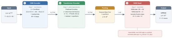
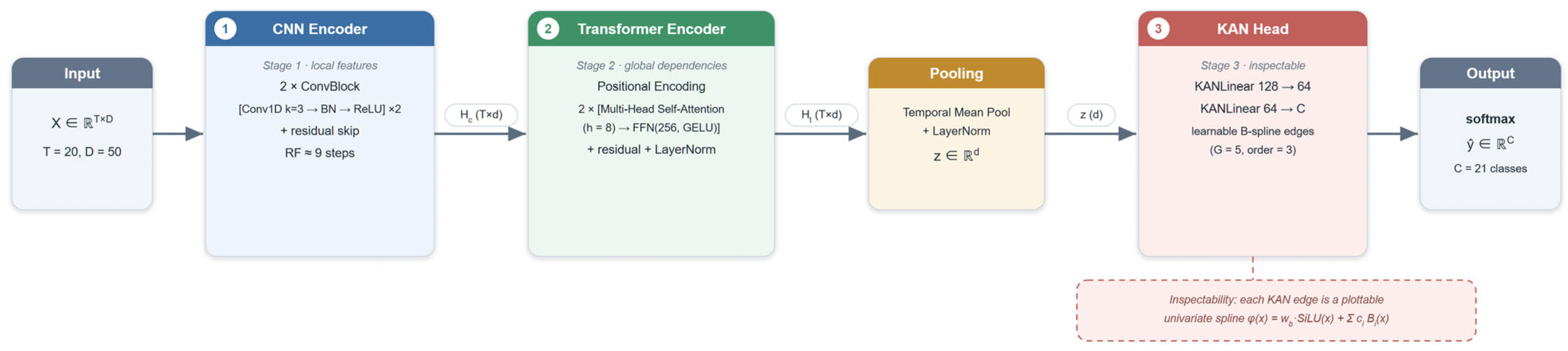
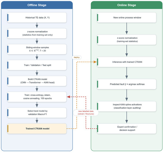
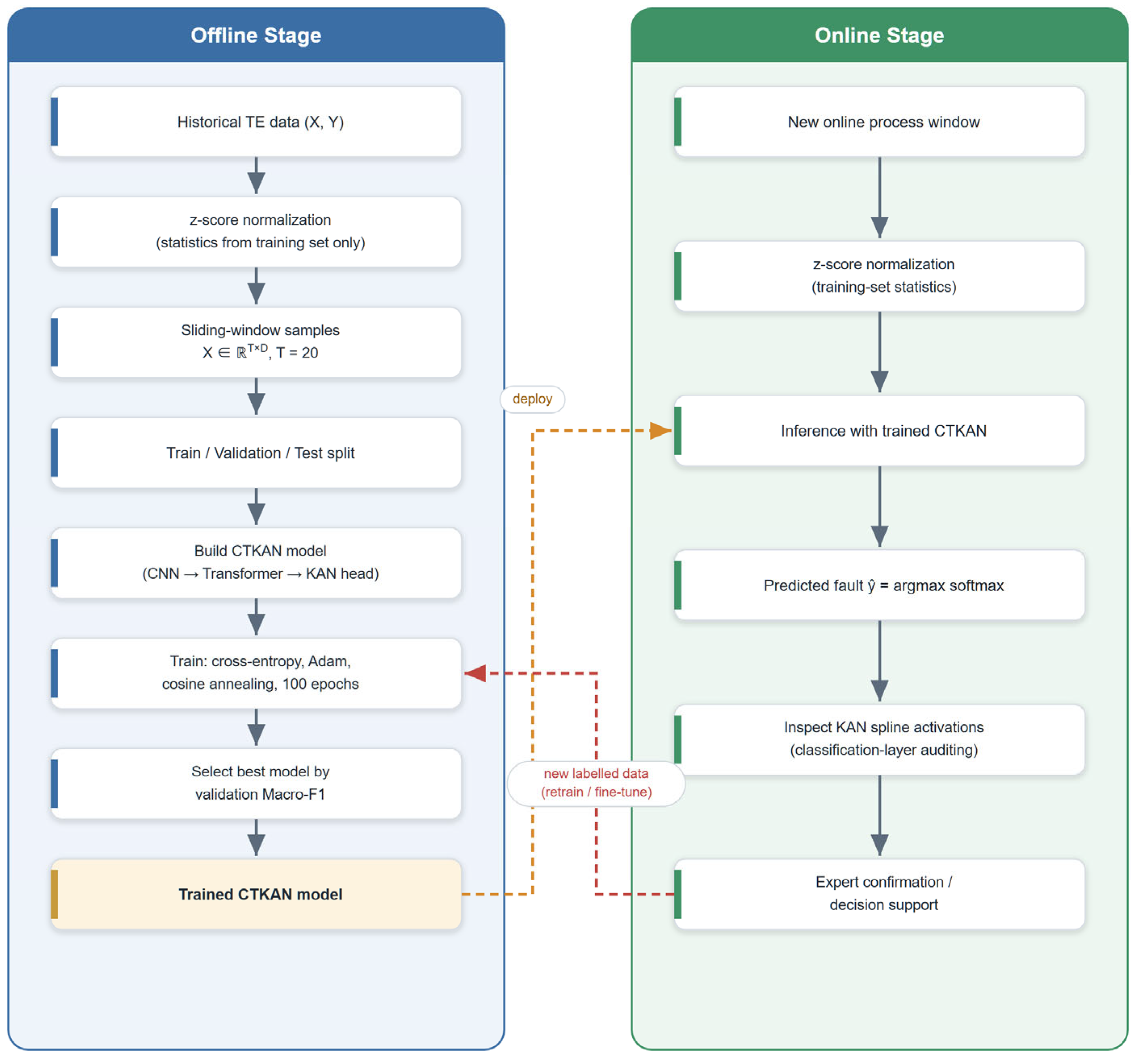
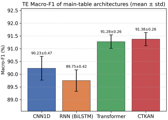
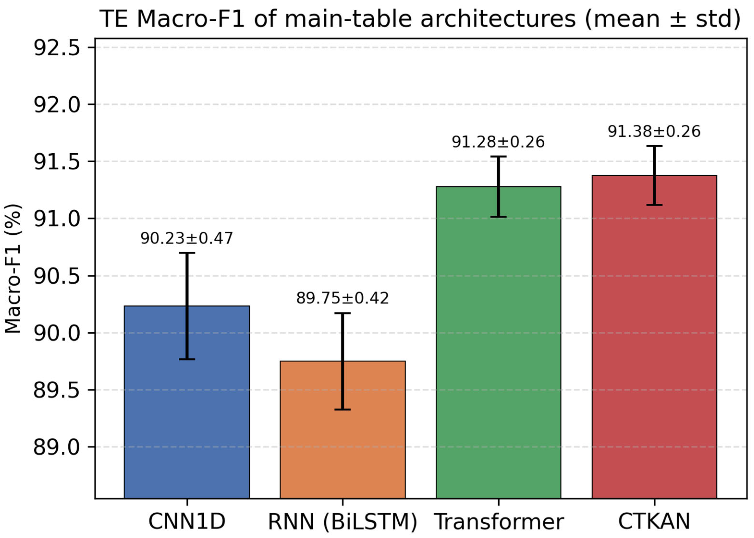
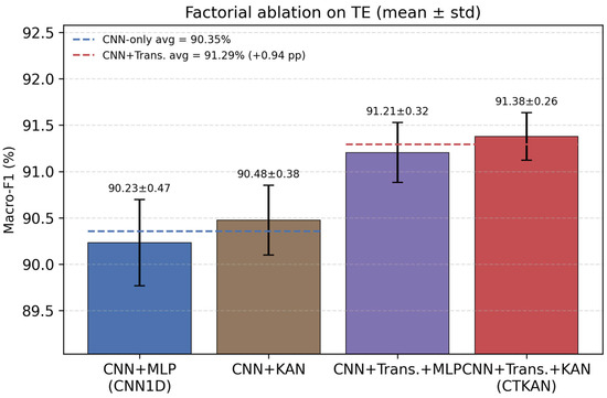
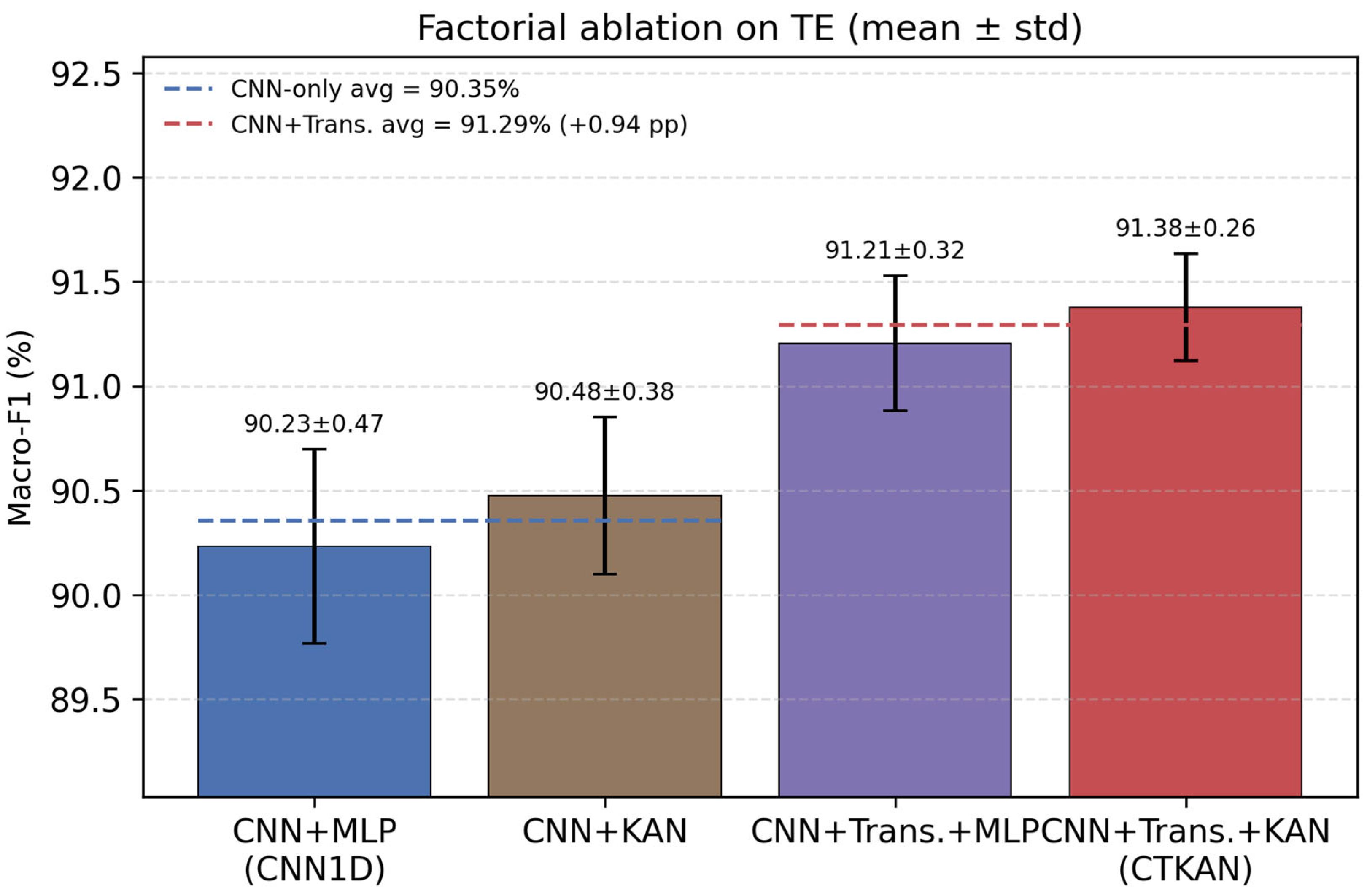
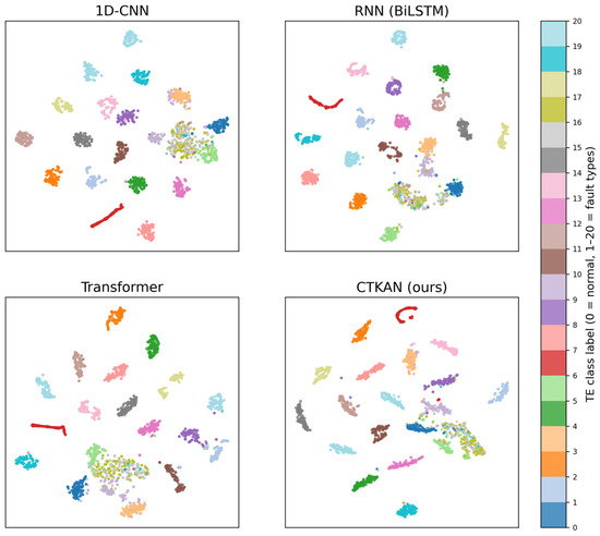
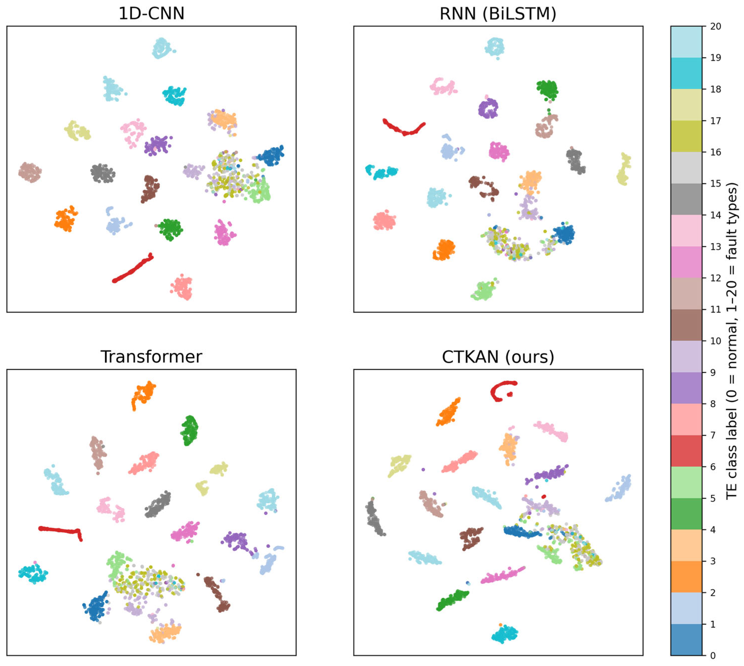
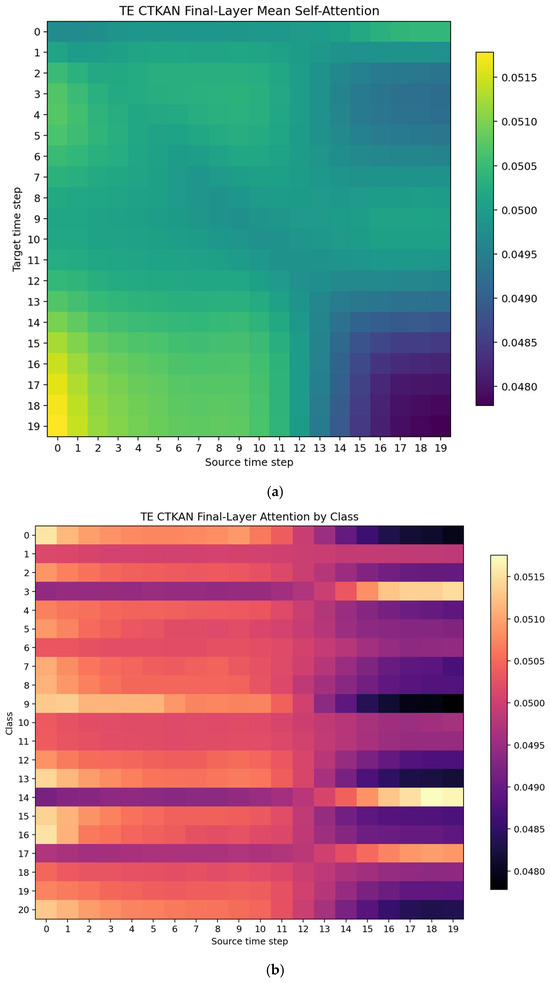
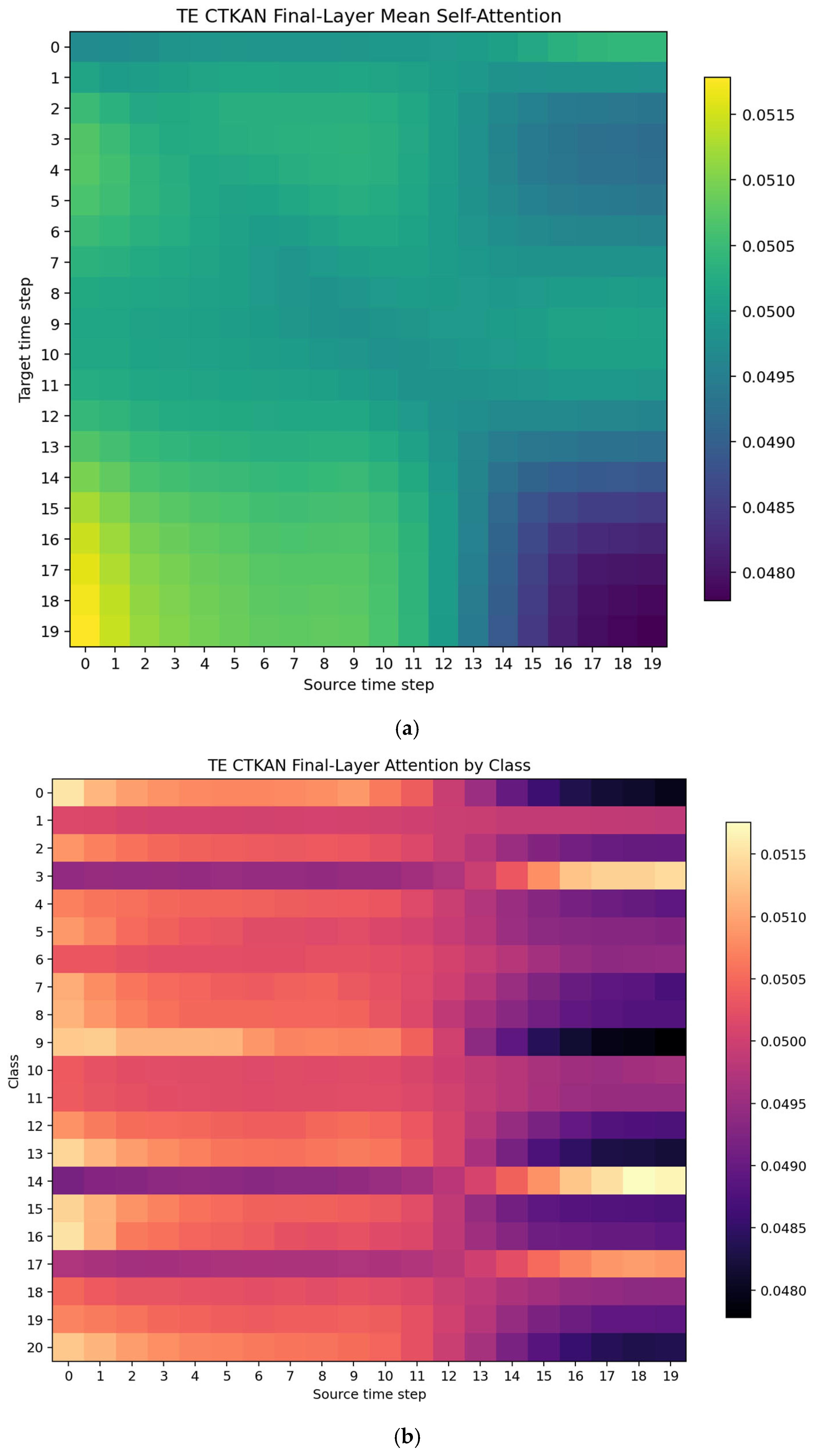
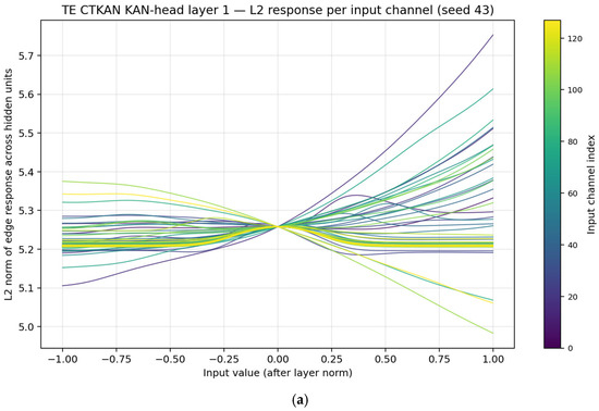
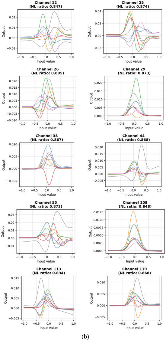
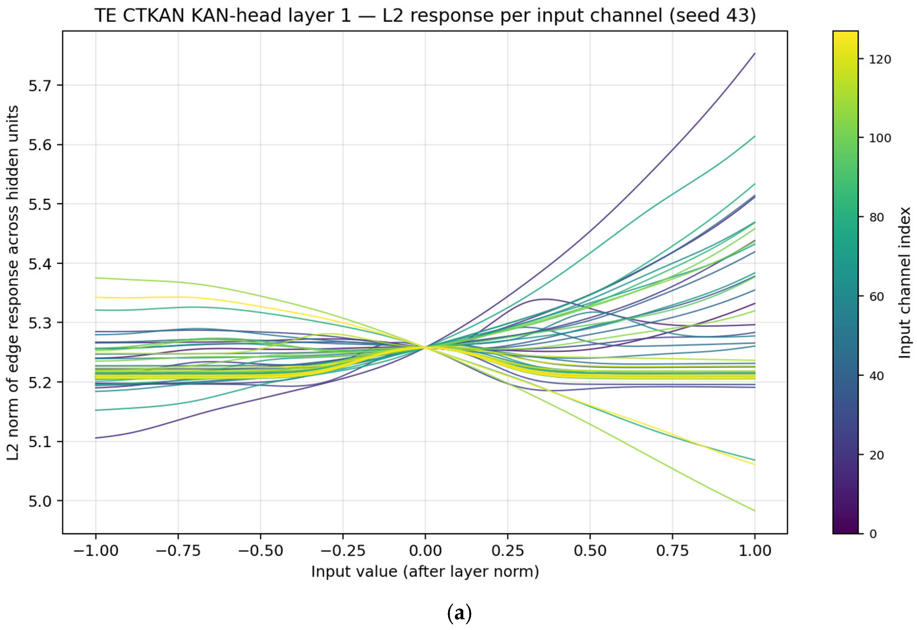
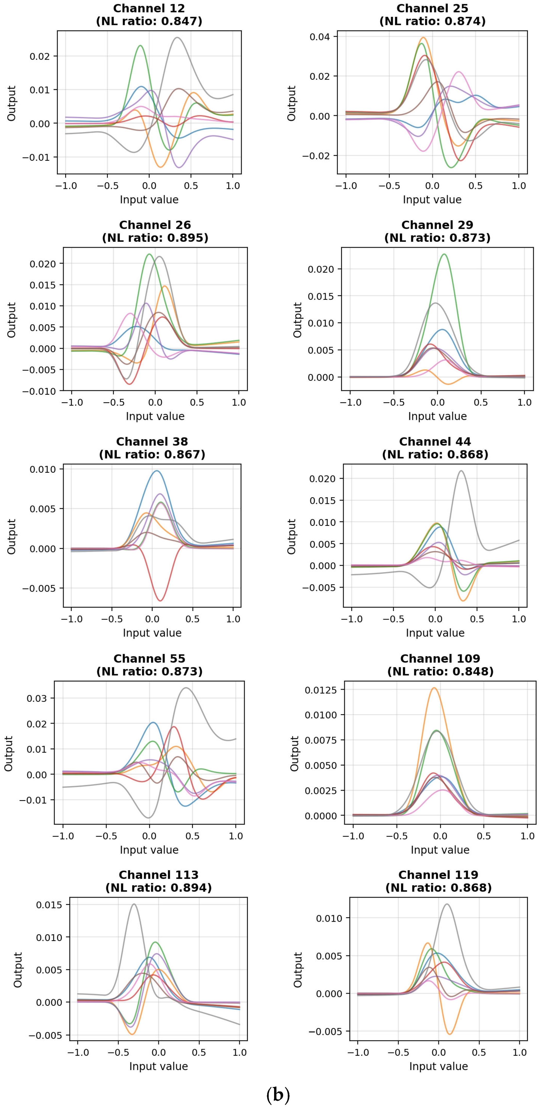
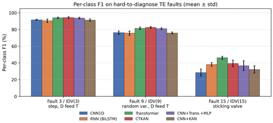
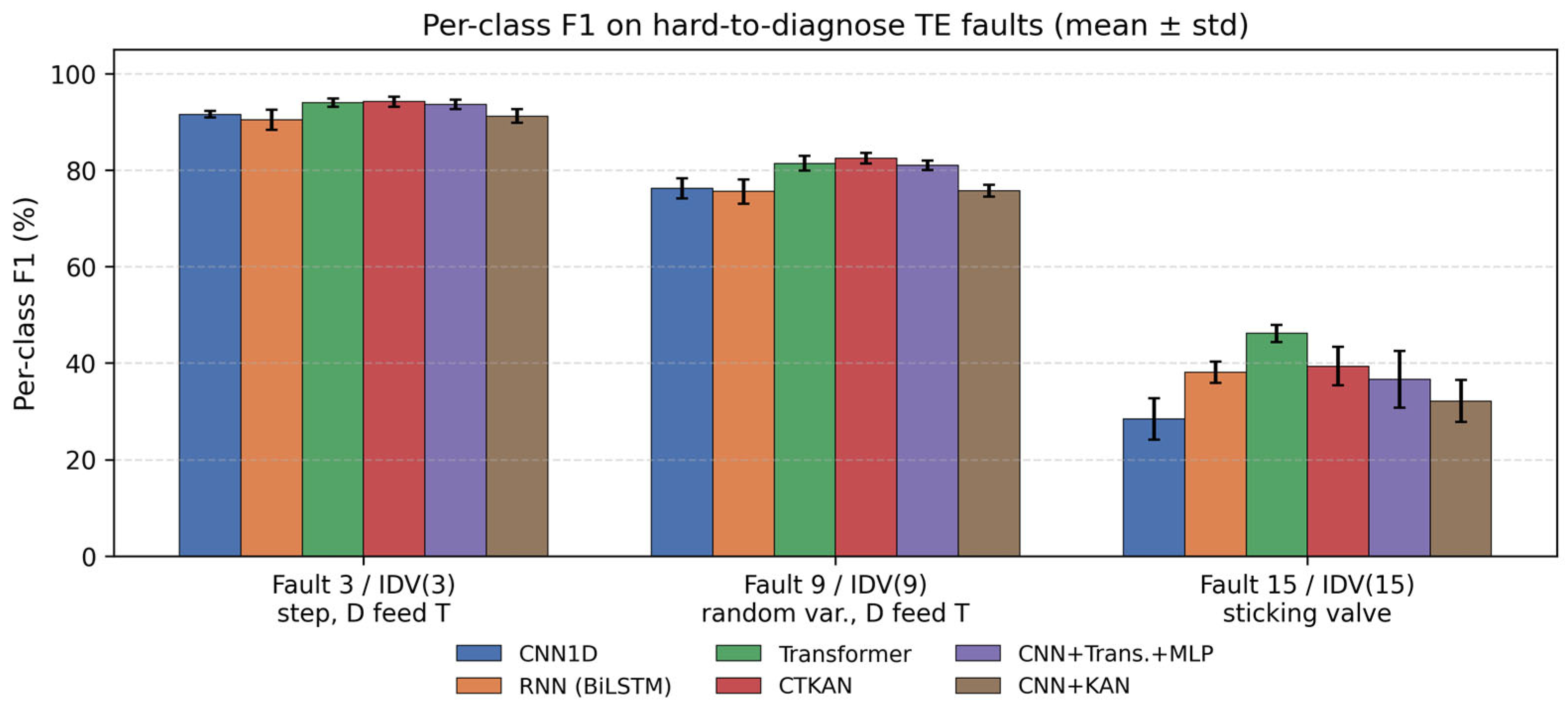
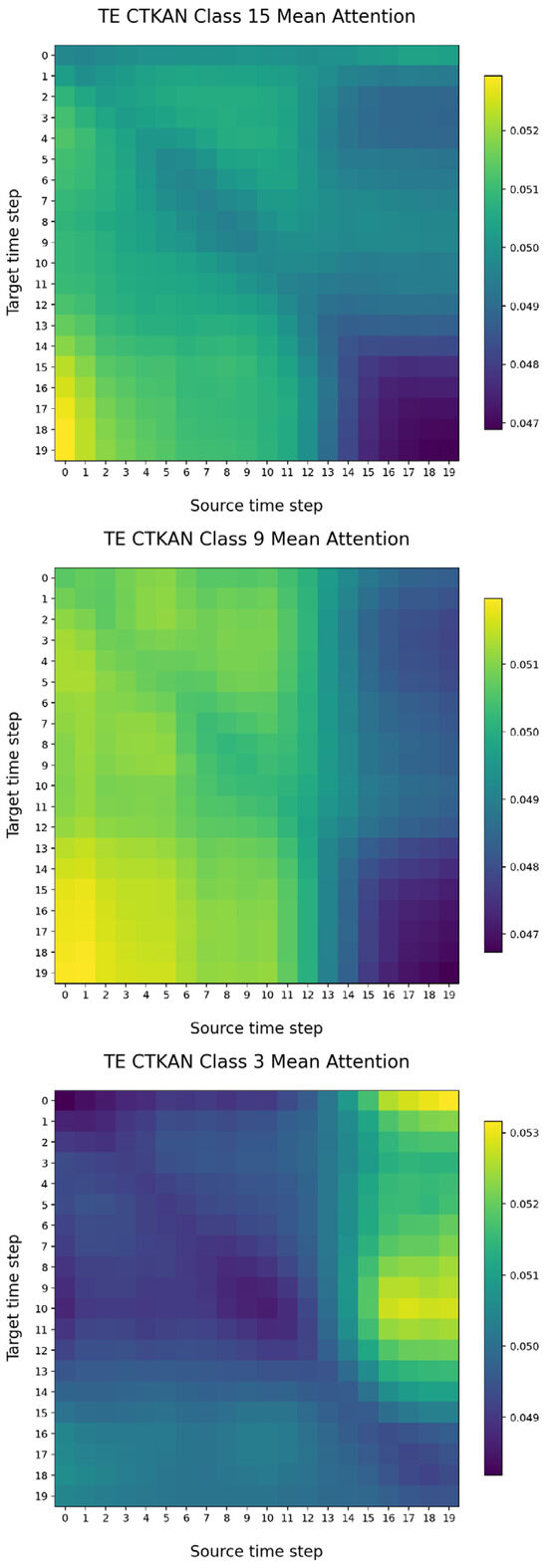
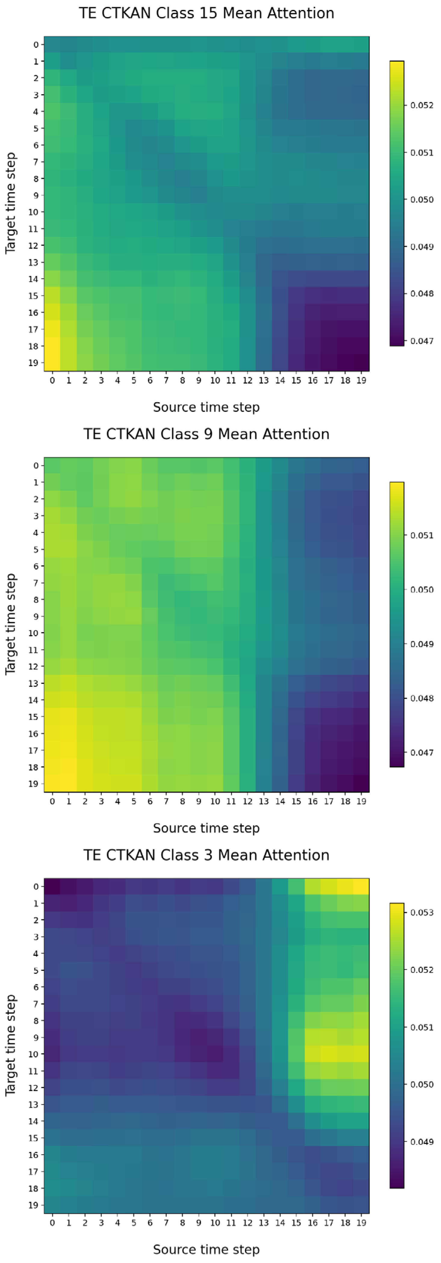
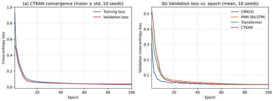
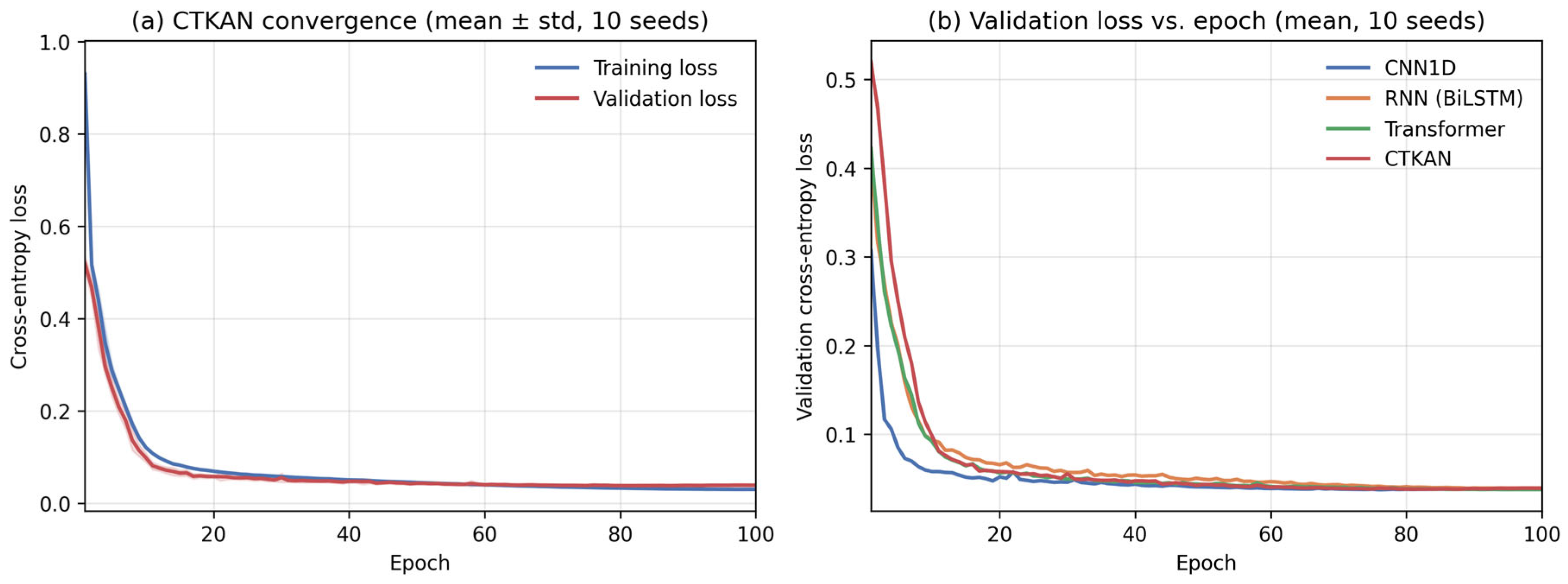
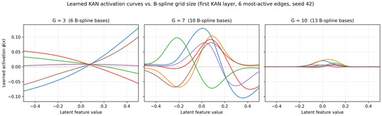
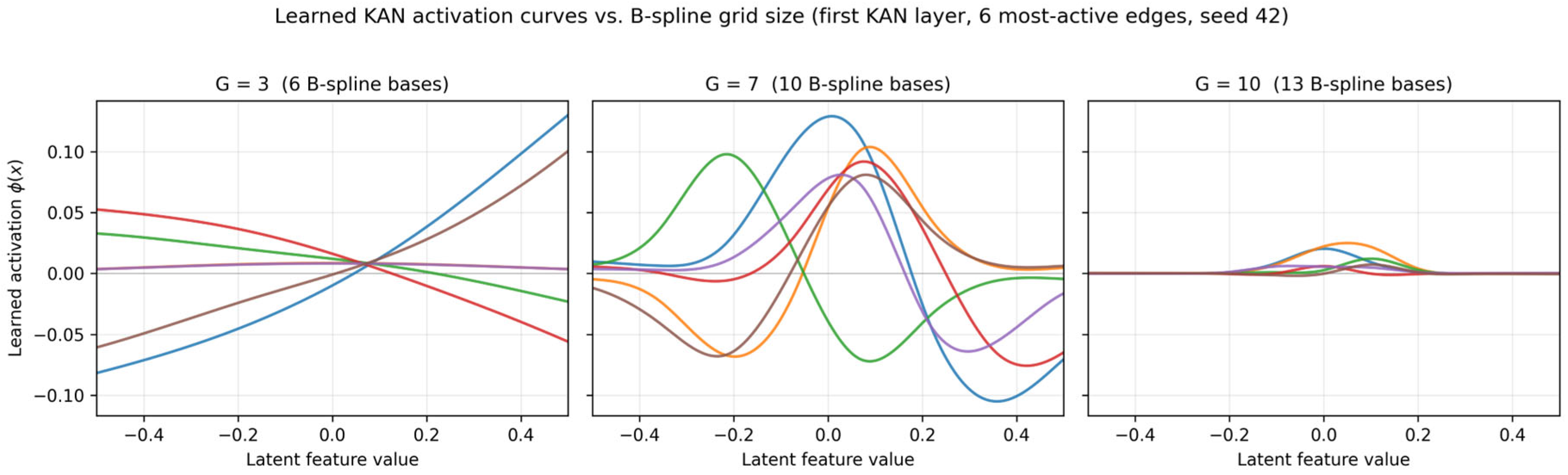
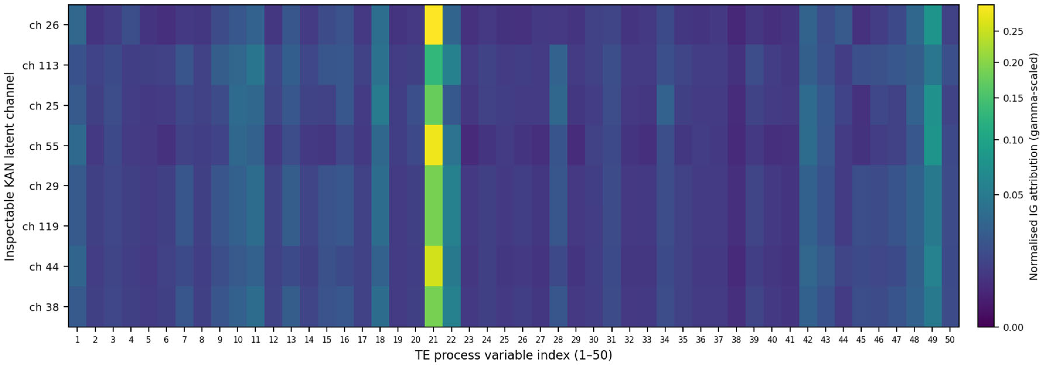

Disclaimer/Publisher’s Note: The statements, opinions and data contained in all publications are solely those of the individual author(s) and contributor(s) and not of MDPI and/or the editor(s). MDPI and/or the editor(s) disclaim responsibility for any injury to people or property resulting from any ideas, methods, instructions or products referred to in the content. |
© 2026 by the authors. Licensee MDPI, Basel, Switzerland. This article is an open access article distributed under the terms and conditions of the Creative Commons Attribution (CC BY) license.