A Crowd Simulation Framework in Special Natural Environments

Abstract

This study introduces a novel crowd simulation framework tailored for special natural environments, such as earthquakes, landslides, and hunting scenarios. The framework integrates continuous dynamics with agent-based mechanisms to model diverse biological cluster interactions effectively. By combining global path planning and local collision detection, it enhances crowd-driven interactions through innovative strategies for path finding, motion, and crowd management. A lightweight 3D reconstruction approach ensures a balance between large-scale simulations, high-fidelity scenarios, and computational efficiency. This framework allows each agent to maintain individual initiative and behavioral diversity, making it highly suitable for large-scale simulations. The proposed model can simulate crowd behavior realistically across various natural scenarios and adapt seamlessly to different environments, offering a robust solution for crowd simulation.

1. Introduction

In human society, densely crowd scenarios such as schools, gatherings, traffic, and construction sites are commonplace in daily activities. In recent years, stampedes on New Year’s Eve, collapses of mines, and schools being severely damaged in earthquakes have occurred from time to time.

The study of crowd dynamics has long been a subject of significant interest, particularly in scenarios where continuous crowds interact in special natural environments. Understanding crowd behavior in such environments is crucial for applications in disaster early warning systems, flood emergency responses, urban planning, village development, and emergency management.

Relevant scholars have already conducted extensive work in large-scale biological cluster (crowd) studies. The current issues that need to be addressed include the following: (1) How do different types of biological clusters interact? (2) How can the authenticity of simulations be further improved? (3) How can a balance be found between large-scale clusters, high-fidelity scenarios, and high-performance computing? (4) How can general algorithms derived from biological cluster (crowd) simulations promote related research?

This paper focuses on these aspects, investigates crowd responses in special natural environments, including earthquakes, landslides, and hunting scenarios, and analyzes crowd and individual behaviors across different conditions. It needs to incorporate various special objects, including biological crowds and solid-state factors to simulate crowd behavior in more diverse natural scenarios.

In this work, we adopt a hybrid approach that unifies continuous dynamics and agent-based mechanisms. We expand the range of agent categories, transitioning from single class to multi-class agents. By integrating the movement of various agents into a unified dynamic force field framework, we incorporate both global path planning and local collision detection into an efficient and streamlined system. This framework enables each agent, despite being influenced by multiple forces, to maintain individual initiative and behavioral diversity, making it suitable for large-scale simulations with high computational efficiency.

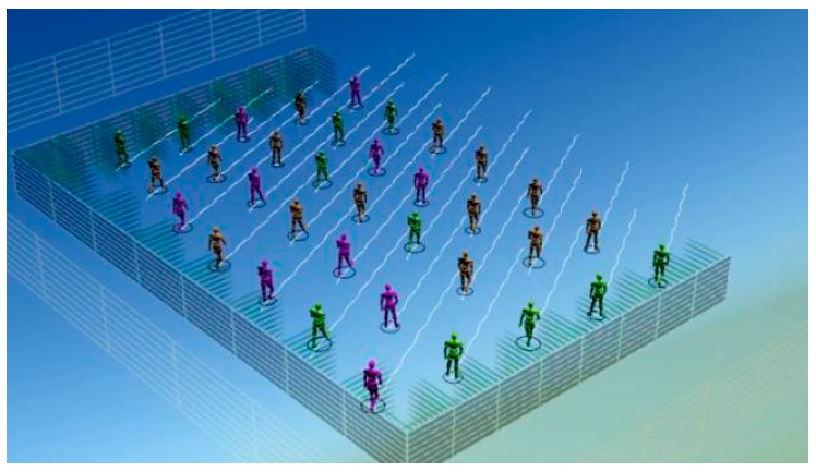
The real scene 3D model in this study collects data from the real world. The scenes in the study need to have practical significance, both from the perspective of measurement and from the perspective of visual effect. This paper extends the framework to cover more complex disaster scenarios, including earthquakes and landslides, by incorporating real-scene 3D modeling through drone-based oblique photography. The resulting elevation, texture, and mesh data are processed using a lightweight 3D reconstruction approach to reduce computational load.

Contributions. Our research introduces several key innovations to achieve realistic crowd simulations in special natural environments. (1) Path finding improvements: inspired by natural phenomena, a Variable-Rotation method is introduced and proposed by enhancing the Minimal-Rotation method. (2) Motion strategies: three novel strategies (Domain Nearest, Domain Farthest and Domain Center methods) are designed based on the collective center approach. (3) Crowd-driven modeling: a Spatial-Extrusion method is proposed to improve crowd-driven interactions within special environments.

Our method can significantly reduce computational overhead, as its cost is mainly influenced by the number of particles. Our system efficiently simulates thousands of particles at a speed of approximately 24 frames per second, or tens of thousands of particles at lower frame rates.

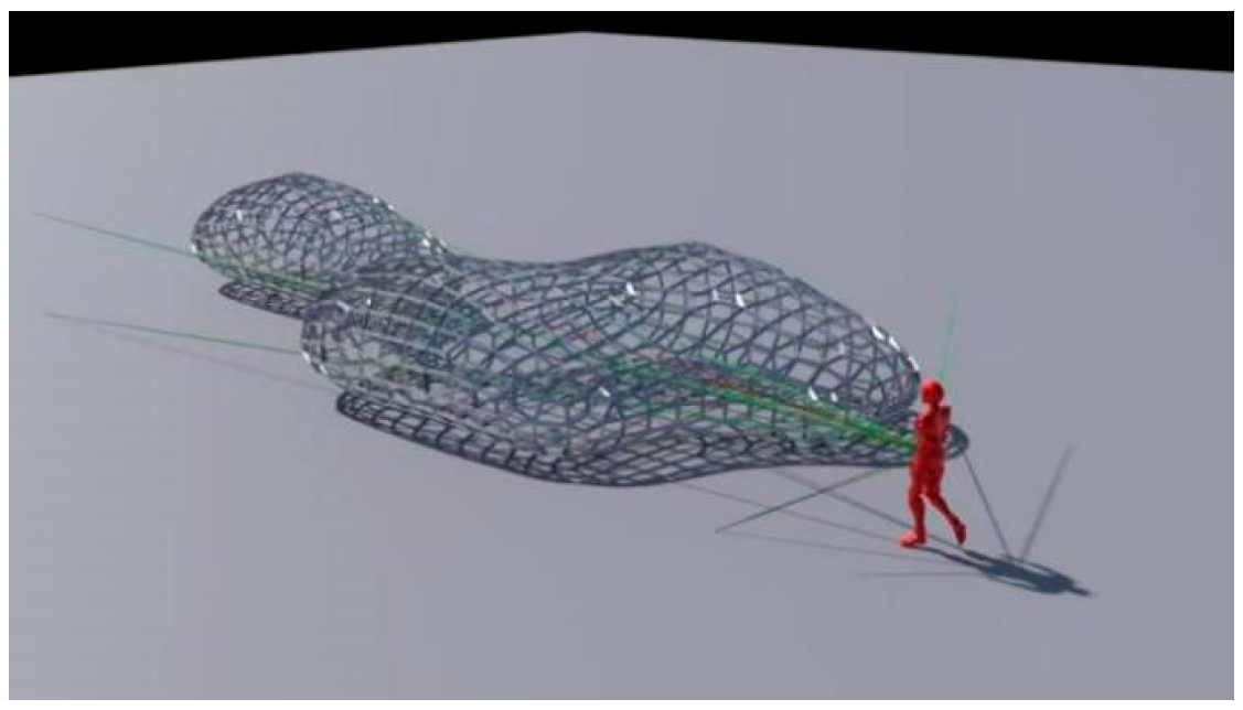
The proposed model effectively simulates crowd behavior in diverse natural scenarios (Figure 1), including earthquakes, hunting, and landslides, and is adaptable to a wide range of environments such as floods, volcanic eruptions and avalanches. The model is also applicable to urban blocks, tunnels and multi-floor indoor spaces with appropriate constraints (e.g., traffic rules and spatial restrictions). By offering a concise and computationally efficient framework, our approach provides a robust means of large-scale crowd simulation across various natural disaster scenarios.

2. Related Works

In this section, we briefly review previous studies relevant to our work. For a more comprehensive overview of crowd simulation research, readers may refer to the literature [1,2].

The foundation of agent-based crowd simulation can be traced back to Reynolds’ seminal work [3], which demonstrated that complex crowd behaviors can emerge from simple local interaction rules. Since then, numerous agent-based models have been proposed, with one of the most well-known being the Social Force Model (SFM) [4]. However, SFM is known to produce oscillatory movement patterns under certain conditions. To mitigate this issue, alternative models have been developed, including velocity-based models [5], vision-based models [6], and learning-based models [7], among others.

Crowd simulation involves not only path planning but also collision avoidance. Early efforts, such as those by Funge et al. [8], explored knowledge-based learning approaches, while Shao and Terzopoulos [9] expanded on these ideas. Various collision avoidance techniques have been proposed, including navigation fields [10], grid-based rules [11], density-dependent techniques [12], particle force interaction models [13], and hybrid long-range collision avoidance models [14], each addressing different aspects of motion coordination in dynamic environments.

Crowd evacuation models have been widely employed to analyze the risks associated with flood scenarios under dynamic emergency conditions. For instance, Shirvani et al. [15,16] utilized hydrodynamic models to simulate crowd evacuation with static scenery assumptions. However, these models primarily focus on computational results and lack applicability for real-time 3D simulations.

More recently, continuum models have been adopted for crowd simulation. Hughes [17] proposed a model in which pedestrians are represented as a continuous density field, with their motion governed by a system of partial differential equations. Treuille et al. [18] introduced a similar potential function approach, guiding pedestrian movement while incorporating “discomfort fields” to account for geographical preferences. Narain et al. [19] further developed a macroscopic continuum model known as the UIC solver. Additionally, some other models [20,21] have been proposed to simulate special crowd behaviors.

In the domain of natural environment modeling, extensive studies have been conducted on disasters such as floods [22], debris flows [23], earthquakes [24,25], and fires [26,27]. These studies primarily focus on disaster assessment, prevention, mitigation strategies, early warning systems, and individual behavior analysis [28,29]. However, most of these works emphasize statistical data analysis, predictive modeling, and scene reconstruction rather than real-time 3D simulation. Notably, the previous work by Zou et al. [30] provided a new solution to crowd evacuation. In this paper, we extend their work by incorporating multiple special types and diverse natural environments, simulating the behavior of heterogeneous crowds in complex scenarios such as earthquakes, landslides, and hunting. Our approach has implications for disaster prevention and mitigation, flood management, urban planning, and risk assessment. By advancing the study of crowd behavior in special natural environments, our approach offers contributes to the forefront of real-time crowd simulation research.

3. Methods

In this section, we introduce the fundamental components of our model, establish precise settings, and extend these principles to group dynamics. We further analyze the interactions between different classes to define the algorithmic foundation. Additionally, we discuss the construction of correlation functions and force fields. The basic entities considered in the model—such as solid types, liquid types, biological clusters, and agents—are driven by force fields and governed by Newton’s laws of motion.

Setting One: At any coordinate point in three-dimensional space, the object’s physical state is described by the following vector quantities:

•

$\overrightarrow{\mathrm{V}}$: The object’s velocity;

•

$\overrightarrow{\mathrm{F}}$: The force acting on the object;

•

$\overrightarrow{\mathrm{X}}$: The object’s position.

Setting Two: The three-dimensional space in the model is partitioned into uniform, continuous cubic cells based on geographical positioning. Terrain and structural features are represented as polygons weighted according to their properties. While polygons may exhibit heterogeneity, all accessible regions must remain continuous.

Setting Three: Let ${\mathrm{vol}}_i$ represent a cubic spatial element and $p{\ln }_i$ denote a planar spatial element. The space is structured as follows:

$$Vol=\left\{vo{l}_0,vo{l}_1,\dots vo{l}_i,vo{l}_j\dots \left.vo{l}_n\right\}\right.$$

(1)

$$voli\cap volj=P{\ln }_{ij}$$

(2)

$$P\ln =\left\{p{\ln }_0,p{\ln }_1,\dots p{\ln }_i,p{\ln }_j\dots \left.p{\ln }_n\right\}\right.$$

(3)

$$p\ln i\cap p\ln j=Lin{e}_{ij}$$

(4)

These definitions establish a structured framework for modeling spatial segmentation and interactions between elements.

The core principle of continuous dynamics is to model motion as a system of interacting particles that influence each other, forming complex motion. Based on density variations, we categorize these types into the following:

•

Solid type: Densely packed entities exhibiting strong inter-molecular forces.

•

Liquid type: Entities with weaker inter-molecular forces, allowing for greater flexibility in motion.

3.1. Forces Computation

The fundamental principle of continuous dynamics is to model the motion of matter as a collection of interacting particles, which collectively generate complex behavior. Due to differences in density, we categorize these into solid type and liquid type. The force calculation formula is as follows:

$$\overrightarrow{F}=m\overrightarrow{a}$$

(5)

Since the mass is determined by its density, it is more practical to use density in place of mass:

$${\overrightarrow{F}}_{replace}=\rho \overrightarrow{a}$$

(6)

The total force acting on a single particle consists of three primary components:

$${\overrightarrow{F}}_{\mathrm{total}}={\overrightarrow{F}}_{external}+{\overrightarrow{F}}_{pressure}+{\overrightarrow{F}}_{viscosity}$$

(7)

where

•

${\overrightarrow{F}}_{\mathit{external}}$ represents external forces, typically gravity, expressed as $\overrightarrow{F}external=\rho \overrightarrow{g}$.

•

${\overrightarrow{F}}_{\mathit{pressure}}$ accounts for pressure-induced forces, defined as ${\overrightarrow{F}}_{pressure}=-\nabla p$. This force moves particles from high-pressure to low-pressure regions and is equal to the gradient of the pressure field.

•

${\overrightarrow{F}}_{viscosity}$ models viscous forces, expressed as ${\overrightarrow{F}}_{viscosity}=\rho {\nabla }^2\overrightarrow{v}$, which arises due to velocity differences among particles and depends on the viscosity coefficient.

Density Computation. The density ρ of a particle is computed using a kernel function. The smooth kernel can be understood as each particle being influenced by other particles within a certain range around it, and the final properties of this particle are determined by the weighted properties of all the surrounding particles:

$$\rho {(x_{\mathrm{i}})=\mathrm{m}{\displaystyle \frac{315}{64\pi h^9}}{{\displaystyle \sum _j(h^2-\left|{\overrightarrow{x}}_i-{\overrightarrow{r}}_i\right|}}^2)}^3$$

(8)

where the smoothing kernel function $W_{\rho }(•)$ takes the following form:

$$W_{\rho }(\overrightarrow{x},h)={\displaystyle \frac{315}{64\pi h^9}}{(h^2-x^2)}^3, (x=\left|\overrightarrow{x}\right|,0\le x\le h)$$

(9)

The research conclusion in Reference [31] proves that the speed and the density of crowd show a linear negative correlation in the roaming state ($\mathrm{V}=1.26-0.28\rho$). This principle is also adopted in the initial setting of the experiment in this paper.

Pressure Computation. The pressure p of a particle is determined using the ideal gas equation:

$$p=k(\rho -{\rho }_0)$$

(10)

where ${\rho }_0$ is the reference static density and k is a constant depending on the properties, such as temperature. In simulating crowd movement, debris flows, and traffic flow, the value of k affects particles’ spacing. Therefore, the value of k should be adjusted experimentally based on the simulated type and experimental outcomes (in this study, the range is ${10}^3~{10}^5$ units). The open-source SPH code documentation explicitly recommends selecting a k value that satisfies $\rho \approx {\rho }_0$, with $k={\rho }_0{c_s}^2$ ($c_s$ is the speed of sound) as the default.

For pressure computation, we adopt the kernel function $W_{\mathrm{p}}(•)$ form as follows:

$$W_P={\displaystyle \frac{15}{\pi {\mathrm{h}}^6}}{(h-x)}^3, x=\left|{\overrightarrow{x}}_i-{\overrightarrow{x}}_j\right|,0\le x\le h$$

(11)

The pressure force exerted on a particle is computed as follows:

$$\begin{array}{l}{\overrightarrow{F}}_{{pressure}_i}=-\nabla p({\overrightarrow{x}}_i)={\displaystyle \frac{45}{\pi h^6}}m{\displaystyle \sum _j\left(\frac{p_i+p_j}{2{\rho }_i{\rho }_j}\frac{{\overrightarrow{x}}_i-{\overrightarrow{x}}_j}{x}{(h-x)}^2\right)},\\ (x=\left|{\overrightarrow{x}}_i-{\overrightarrow{x}}_j\right|,0\le x\le h,m\equiv m_j)\end{array}$$

(12)

Viscosity Computation. The force due to viscosity can be derived similarly. Since velocity imbalances cause viscosity effects, we substitute relative velocity into the following formula:

$${\overrightarrow{\mathrm{F}}}_{{\mathrm{viscos}ity}_i}=\mu m{\displaystyle \frac{45}{\pi h^6}}{\displaystyle \sum _j\frac{{\overrightarrow{v}}_i-{\overrightarrow{v}}_j}{{\rho }_j}}(h-\left|{\overrightarrow{x}}_i-{\overrightarrow{x}}_j\right|)$$

(13)

where μ is the viscosity coefficient. The viscosity coefficient is a key parameter describing the viscous behavior of fluids, and its value depends on the type of fluid and physical conditions (e.g., the viscosity coefficient of water at 20 °C is about 0.001 Pas, and that of oil may be as high as 1 Pas or more). The corresponding kernel function $W_{\mathrm{v}}(•)$ is defined as follows:

$$W_v(\overrightarrow{x},h)={\displaystyle \frac{15}{2\pi h^3}}(-{\displaystyle \frac{x^3}{2h^3}}+{\displaystyle \frac{x^2}{h^2}}+{\displaystyle \frac{h}{2x}}-1),(x=\left|{\overrightarrow{x}}_i-{\overrightarrow{x}}_j\right|,0\le x\le h)$$

(14)

This formulation ensures a comprehensive representation of the force computation, capturing external forces, pressure dynamics, and viscosity effects in a physically consistent manner.

3.2. Global Path Planning

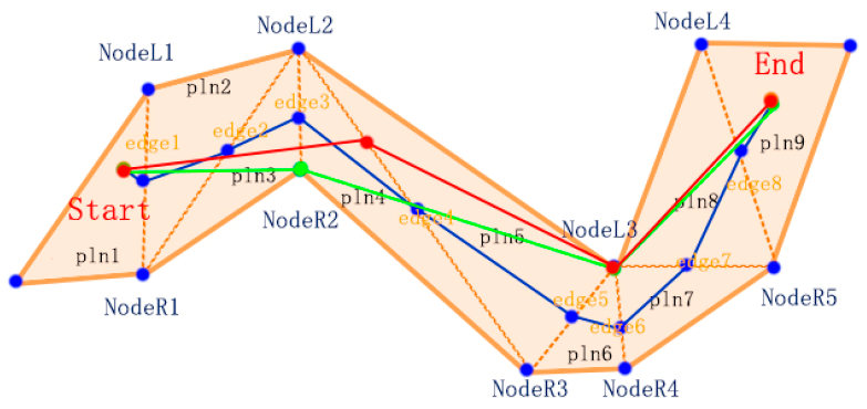
A previous work [30] introduced a Minimal-Rotation Method (the main ideal of which is to ensure that the agent moves towards the destination with the minimum total rotation angle) for a convex polygon path-finding algorithm. In this section, we improve and optimize this algorithm. As illustrated in Figure 2 (where the blue line is the midpoint method, the green line is inflection point method [32], and the red line is minimal-rotation path planning method [30]), agents determine their optimal paths based on the zones they occupy. The path from the start location to the end location consists of a sequence of polygons, where each pair of adjacent polygons shares exactly one intersecting segment.

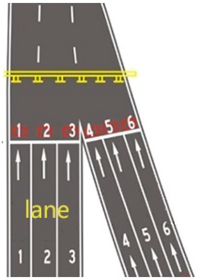
Inspired by real-world traffic scenarios, we propose an improved approach. As illustrated in Figure 3, vehicles in the rightmost lane (Lane 3) should ideally move straight or turn right based on the minimal-rotation principle. However, in the case of merging vehicles on the right side, turning left to Lane 2 may be the safer option. Motivated by this observation, we introduce variations to the original algorithm to account for dynamic factors such as crowd density, terrain elevation, and passageway availability. This leads to the Variable-rotation path-finding method described below.

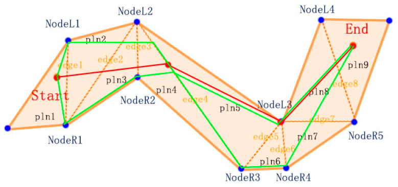
Variable-rotation Path Finding Method (Figure 4). (1) Initialize an empty tracking queue. (2) Connect the starting point to the endpoint to form the to-target line. (3) Identify the first internal edge that intersects the to-target line and compute the intersection point. (4) Compare the weighted values of three candidate points: the left endpoint, the intersection point, and the right endpoint. (5) Select the point with the lowest weight (based on a function of angle and distance) and append it to the tracking queue. (6) If no internal edge intersects the to-target line, compute the angles between the line and both endpoints of the closest internal edge, selecting the one with the minimal weighted value. (7) Repeat steps 2–6 until the tracking queue is empty. The specific algorithm is shown in Algorithm 1.

Algorithm 1. The Variable-rotation Path Finding Method

For a given convex polygon, there are: $\begin{array}{l}P\ln s=\left\{p{\ln }_1,\dots p{\ln }_i,p{\ln }_j\dots \left.p{\ln }_n\right\}\right.\\ p\ln i \mathrm{adjoin} p\ln j,p\ln i\cap p\ln j=edg{e}_i\\ Edges=\{edg{e}_1\dots edg{e}_i\dots edg{e}_n\}\\ (leftPo{\mathrm{int}}_i,rightPo{\mathrm{int}}_i)\equiv endpo\mathrm{int}\in edg{e}_i,\\ LeftPo\mathrm{int}s=\{leftPo{\mathrm{int}}_1\dots leftPo{\mathrm{int}}_i\dots leftPo{\mathrm{int}}_n\}\\ RightPo\mathrm{int}s=\{rightPo{\mathrm{int}}_1\dots rightPo{\mathrm{int}}_i\dots leftPo{\mathrm{int}}_n\}\\ TracePo\mathrm{int}s=\left\{Start\right\}\end{array}$ The starting point is: Start, and the end point is: End. FindNextTracePoint(TracePoints,Edges,End) Input:TracePoints,Edges,End Output:Path Select First P ⊂ TracePoints Make Line L_Start_To_End Find Nearest edgei If(L_Start_To_End intersect with edgei) { Calculate the intersection: cross_point_i;

For each point in {leftPointi, cross_point_i, rightPointi} $\mathrm{Min} \mathrm{Weight}\mathrm{P}\leftarrow Min({\mathrm{Linear}(\mathrm{W}}_{\mathrm{rot}}\times {\theta }_{rot}+{\mathrm{W}}_{\mathrm{dist}}Le{n}_{dist}))$ End $\mathrm{Trace} \mathrm{Point}\leftarrow \mathrm{MinWeightP}$ } Else { For each point in {leftPointi, rightPointi} $\mathrm{Min} \mathrm{Weight}\mathrm{P}\leftarrow Min({\mathrm{Linear}(\mathrm{W}}_{\mathrm{rot}}\times {\theta }_{rot}+{\mathrm{W}}_{\mathrm{dist}}Le{n}_{dist}))$ End $\mathrm{Trace} \mathrm{Point}\leftarrow \mathrm{MinWeightP}$ } If TracePoints !=Null Return Step:FindNextTracePoint Else Return Final Path End

The weight function for selecting the optimal tracking point is given by

$$\mathrm{TraceP}=Min({\mathrm{Linear}(\mathrm{W}}_{\mathrm{rot}}\times {\theta }_{rot}+{\mathrm{W}}_{\mathrm{dist}}Le{n}_{dist}))$$

(15)

where $\mathrm{TraceP}$ represents the final selection of tracking point, $\mathrm{Linear}$ represents the linear interpolation function, ${\mathrm{W}}_{rot}$ denotes the weight of rotation angle, ${\theta }_{rot}$ denotes the rotation angle, ${\mathrm{W}}_{dist}$ denotes the distance’s weight, and $Le{n}_{dist}$ denotes the distance’s length. The default weight values ${\mathrm{W}}_{rot}$ and ${\mathrm{W}}_{dist}$ are set as 0.5 in experiments.

The introduced Variable-rotation method retains the advantages of the Minimal-rotation approach while significantly enhancing flexibility. It adapts to dynamic external conditions such as density variations, terrain slopes, and traffic regulations with minimal additional computational cost.

3.3. Local Routing Strategy

During the process of local routing, people may encounter many changes, especially in the event of sudden situations such as earthquakes, landslides, and floods. The local space where the crowd is located may experience significant environmental changes, and there will be many situations where internal particle forces cannot drive, such as falling objects from high altitudes, vehicles coming from the side, and pedestrians walking against the flow. In such cases, it is necessary for individuals to adopt local strategies to cope.

The following strategies are adopted for individuals:

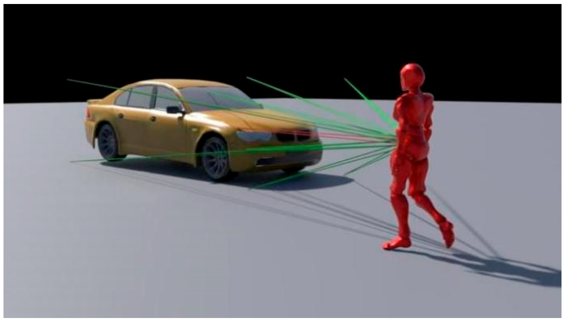
Strategy One 1 vs. 1: When an individual encounters a single incoming object in three-dimensional space (based on relative velocity), the following steps are taken: (1) Compute the line connecting the centroid of the individual to the centroid of the incoming object, called centroid-line. (2) Compute the lines connecting the centroid of the individual to the vertices of the bounding box of the incoming object, called boundary-lines. (3) Calculate the angles between the centroid-line and the boundary lines in eight possible directions. (4) Select the boundary-line with the smallest escape angle as the preferred direction for movement (Figure 5).

Strategy Two 1 vs. n: When multiple objects are incoming in three-dimensional space, the following steps are taken: (1) Generate a bounding grid encompassing all incoming objects, treating them as a single entity. (2) Compute the centroid-line and boundary-lines using the bounding grid instead of an individual object. (3) Calculate the escape angles and select the smallest one for movement (Figure 6).

The following four strategies are those adopted when individuals are in crowd mode.

Strategy Three n vs. 0: When a crowd is in a roaming or migrating state, the following steps are taken: (1) Each individual calculates the direction ${\overrightarrow{\mathrm{N}}}_{self->\mathrm{pa}th}$ toward the target (e.g., the nearest point on a path or center point of the group). (2) This computed direction becomes the primary movement vector (Figure 7).

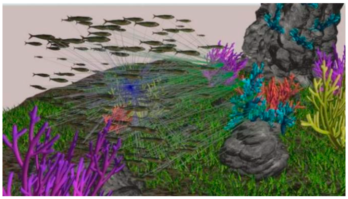
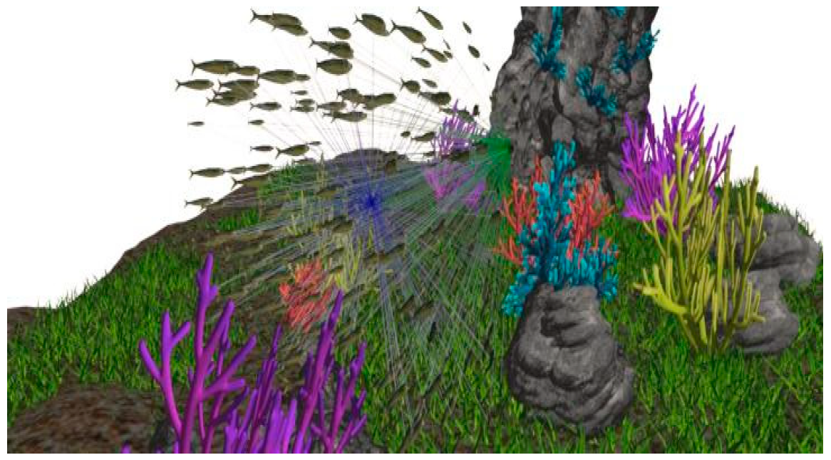
Strategy Four n vs. 1: When a crowd is engaged in foraging or hunting, the following steps are taken: (1) Each individual calculates the direction ${\overrightarrow{\mathrm{N}}}_{self->\mathrm{target}}$ toward the target. (2) This direction is taken as the primary movement vector (Figure 8).

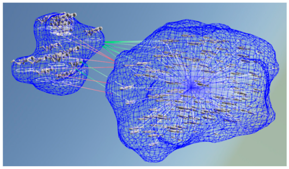
Strategy Five n vs. m: In a competitive or defensive scenario between two crowds (A vs. B), the following steps are taken: (1) Each individual in crowd A (upon reaching a threshold distance) calculates the direction to its crowd’s centroid and the direction to the nearest individual in crowd B. (2) Movement follows a random trajectory along the difference between these two directions to introduce unpredictability (Figure 9).

Strategy Six n_domain vs. m (The Neighborhood Extremum Method): A domain-aware version of the above Strategy Five, where the following steps are taken: (1) Individual a (upon reaching a threshold distance) considers only interactions within a local neighborhood (core-radius ra). (2) Compute movement based on a combination of center, nearest, or farthest points in the neighborhood relative to the opponent. The specific algorithm is shown in Algorithm 2 and Figure 10.

Algorithm 2. Strategy Six ndomain Vs m (The Neighborhood Extremum Method).

For a given convex polygon, there are: $\begin{array}{l}P\ln s=\left\{p{\ln }_1,\dots p{\ln }_i,p{\ln }_j\dots \left.p{\ln }_n\right\}\right.\\ p\ln i \mathrm{adjoin} p\ln j,p\ln i\cap p\ln j=edg{e}_i\\ Edges=\{edg{e}_1\dots edg{e}_i\dots edg{e}_n\}\\ (leftPo{\mathrm{int}}_i,rightPo{\mathrm{int}}_i)\equiv endpo\mathrm{int}\in edg{e}_i,\\ LeftPo\mathrm{int}s=\{leftPo{\mathrm{int}}_1\dots leftPo{\mathrm{int}}_i\dots leftPo{\mathrm{int}}_n\}\\ RightPo\mathrm{int}s=\{rightPo{\mathrm{int}}_1\dots rightPo{\mathrm{int}}_i\dots leftPo{\mathrm{int}}_n\}\\ TracePo\mathrm{int}s=\left\{Start\right\}\end{array}$ The starting point is: Start, and the end point is: End. FindNextTracePoint(TracePoints,Edges,End) Input:TracePoints,Edges,End Output:Path Select First P ⊂ TracePoints Make Line L_Start_To_End Find Nearest edgei If(L_Start_To_End intersect with edgei) { Calculate the intersection: cross_point_i;

For each point in {leftPointi, cross_point_i, rightPointi} $\mathrm{Min} \mathrm{Weight}\mathrm{P}\leftarrow Min({\mathrm{Linear}(\mathrm{W}}_{\mathrm{rot}}\times {\theta }_{rot}+{\mathrm{W}}_{\mathrm{dist}}Le{n}_{dist}))$ End $\mathrm{Trace} \mathrm{Point}\leftarrow \mathrm{MinWeightP}$ } Else { For each point in {leftPointi, rightPointi} $\mathrm{Min} \mathrm{Weight}\mathrm{P}\leftarrow Min({\mathrm{Linear}(\mathrm{W}}_{\mathrm{rot}}\times {\theta }_{rot}+{\mathrm{W}}_{\mathrm{dist}}Le{n}_{dist}))$ End $\mathrm{Trace} \mathrm{Point}\leftarrow \mathrm{MinWeightP}$ } If TracePoints !=Null  Return Step:FindNextTracePoint Else  Return Final Path End

The above strategies from 1 to 5 are similar to the strategy proposed in reference [3]; however, the strategies in this paper are based on a hybrid model, while reference [3] is based on a single model (

Table 1. Strategy comparison between this paper and reference [3].

Feature Model Name	Reynolds’ Boids Strategies	Reynolds’ Steering Behavior Strategies	The Equivalent Strategies of This Paper
Drive mode	Agent-based	Agent-based	Hybrid SPH and Agent
Key distinction	It focuses on the self-organizing (emergent) behaviors of the cluster.	Focus on individual navigation.	It aims to solve the self-organizing (emergent) behaviors of mixed clusters and the multi-level spatial navigation of individual.
Advantage	Easy to implement and the cluster behavior is realistic.	Supports 2D/3D models with plug-in behavior modules.	Individual strategies and group strategies are integrated.
Limitation	Cannot handle complex obstacles.	Single drive mode.	High computational overhead.
Application scenarios	Suitable for single cluster, such as bird or fish animations.	Suitable for simulating realistic movements of autonomous characters in game AI.	Suitable for mixed clusters and various natural environments (e.g., landslide, undersea, urban blocks, tunnels, multi-floor indoor spaces).

). Strategy 6 is innovation strategy, which we propose based on real-world observations.

3.4. Related Algorithms

Here, we introduce a Spatial-Extrusion method to improve crowd-driven interactions within confined environments.

Spatial-extrusion method. The so-called spatial-extrusion method (Figure 11 and Figure 12) is that when the crowd is in a confined space with limited exits, the spatial-extrusion method applies pressure from an inner spot (or anywhere) to the crowd to drive the group movement, just like the way we squeeze toothpaste in real life. In the real world, when disasters occur, they are often accompanied by the collapse of space.

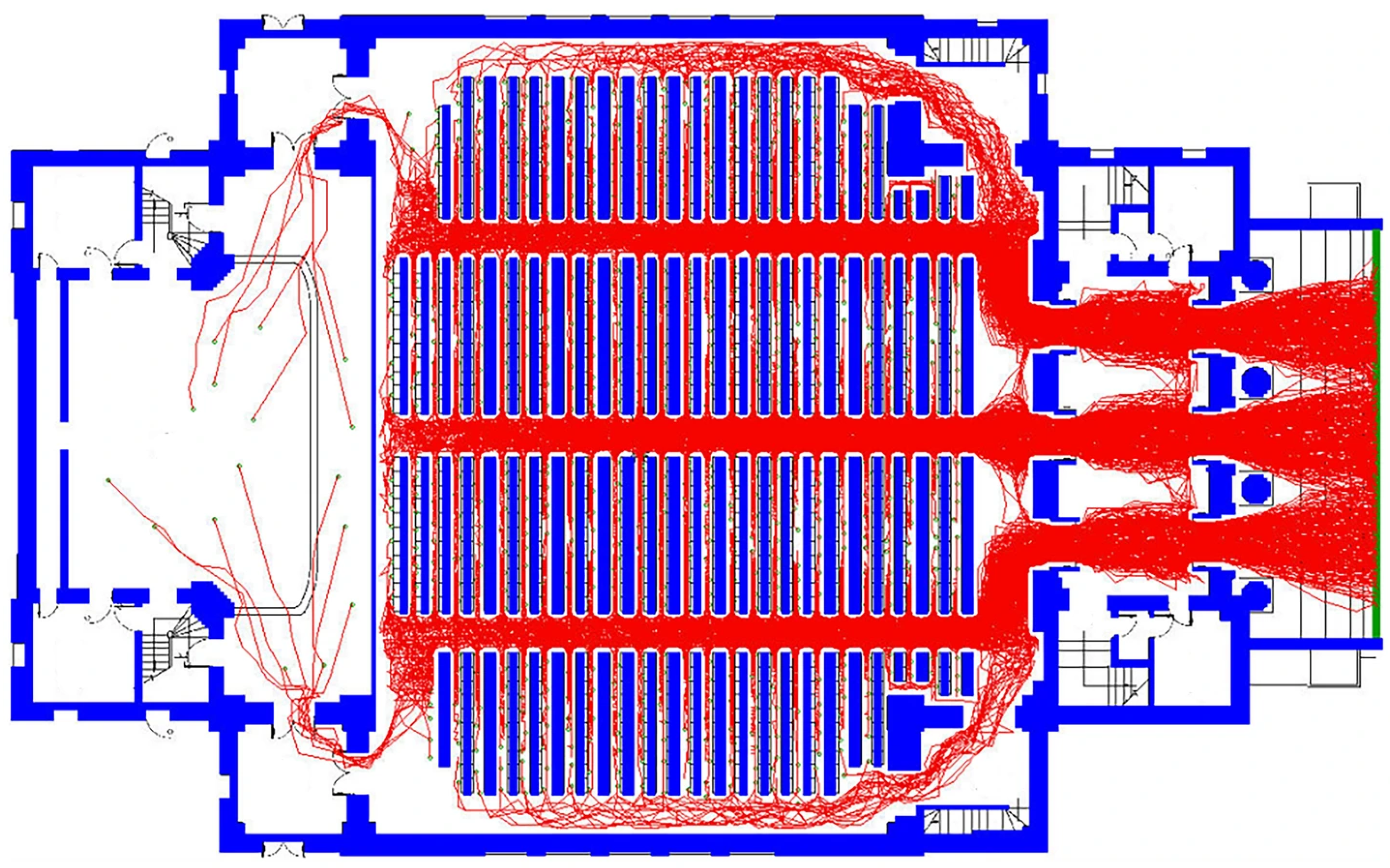
The simulation experiments in the literature [31] also modeled the evacuation of people in a confined exit space (based on potential energy field and other methods). However, the experiment results of the literature [31] do not provide real-time 3D visualization (Figure 13).

4. Implementation Details

To validate the algorithms and strategies discussed above, we construct three experimental scenarios: earthquake, landslide and fishing in water. To ensure authenticity in the experimental setup, we utilize oblique photography data for scene reconstruction in the first two scenarios. The fishing scenario is designed to reproduce natural observations.

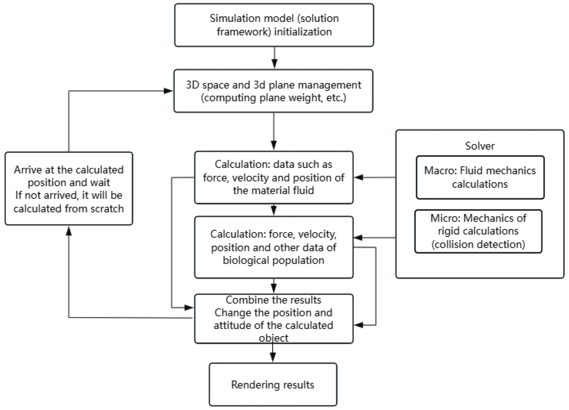
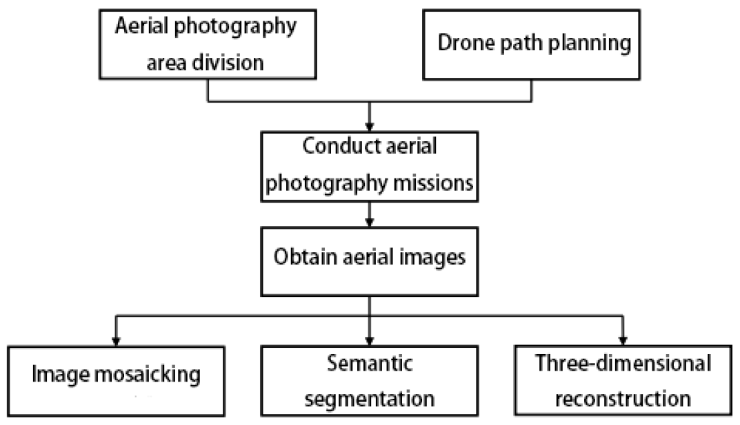
As shown in Figure 14, the simulation model (solving framework) operates in each time unit according to the following process. The process of oblique photography data collection in this study is shown in Figure 15 (taking measured data from a specific district in a city of Jiangxi Province as an example, with the collection date in May 2024).

We employ oblique photography (part data) to capture target images synchronously from one vertical and four oblique perspectives. This process provides high-resolution texture and altitude data, which we then use to construct the scene mesh. The aerial imaging model used is the CTI P330Pro drone, with the following specifications: ground resolution: 2 cm; ground control point interval: 1 km; flight altitude: 178 m; route spacing: 48 m; sampling interval: 21 m.

The specific implementation methods and processes discussed in this section will be elaborated upon in future studies. Below, we take a campus scene as an example of the reconstruction process.

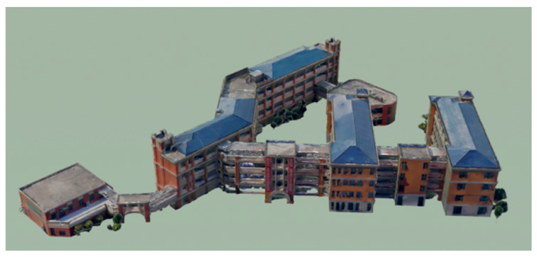
Scene Importing. Our original data consists of tile blocks of size 50 m × 50 m (see Figure 16a). The existing dataset is a textured mesh containing over one million points and nearly ten million vertices. To process this data efficiently, we perform the following preliminary steps: (1) Clipping-Extracting the relevant section of the scene. (2) Stitching-Merging adjacent tiles. (3) Reduction-Decreasing data complexity. (4) Denoising-Removing unwanted noise artifacts. The result is shown in Figure 16b,c.

As shown in

Table 2. Scene data comparison chart.

Data Operation	Points	Polygons	Vertices
Original data	4,671,744	7,805,565	23,416,695
Cropped data	1,577,905	2,967,147	9,287,655
After reduction	142,857	296,307	980,027

, after preprocessing, the scene data volume is reduced by a factor of ten, significantly optimizing computational efficiency.

Ground separation. Following scene import and data cleaning, we obtain a complete grid. To simulate earthquake effects, we extract building structures from the ground and separate their features (Figure 17).

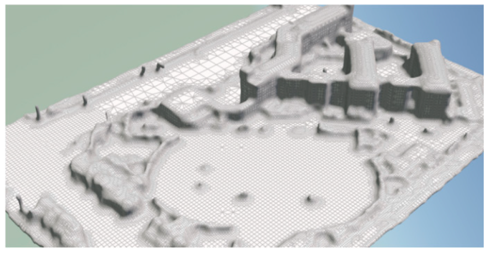
Low-resolution mesh construction. Despite preprocessing, the dataset remains computationally intensive, consisting of hundreds of thousands of points and polygons. Using this raw data directly would lead to significant time costs. To optimize computation, we generate a low-resolution mesh (Figure 18).

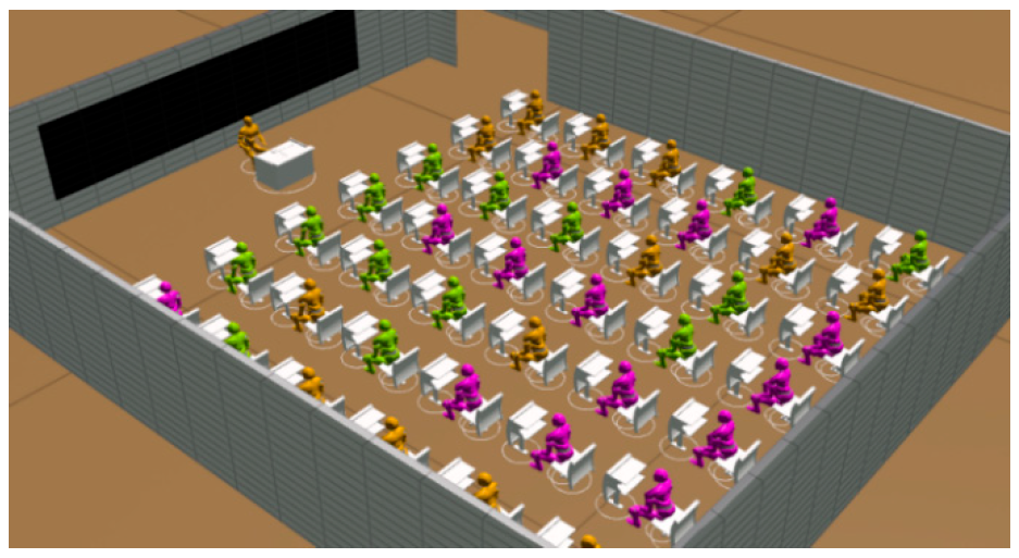
Sub-scene construction. For indoor environments, the presence of homogeneous objects (e.g., tables, chairs) presents a challenge. To efficiently simulate these environments, (1) we treat homogeneous solids as particle-based solid type. (2) These particles are integrated with crowd simulations, allowing for interactions between biological and solid-state type (Figure 19). A similar multi-particle fusion approach is applied for modeling interactions between crowds, vehicles, and debris (Figure 1c).

Three-dimensional model space setting. According to the Human Dimensions of Chinese Adults [33], the 95% maximum shoulder width and chest thickness for adult men are 46.9 cm and 24.5 cm, respectively, while those for adult women are 43.8 cm (maximum shoulder width) and 23.9 cm (body thickness). To more accurately model crowd micro-behavior, this study defines the three-dimensional space occupied by a human body as 50 cm × 30 cm × 170 cm (width, thickness, height), designated as 1 space unit. Tables and chairs are assigned 0.5 units, fishes 0.05 units, and vehicles 10 units, with stochastic variations incorporated where applicable.

5. Results

The experiments were conducted on a PC equipped with an Intel (R) Core (TM) i9-14900KF 3.20 GHz CPU, NVIDIA GeForce RTX 4090 GPU, and 64GB RAM. The algorithm was implemented using Python 3.9 within the Houdini environment. The experiment ran stably at a speed of 24 FPS. The primary objectives of our implementation include (1) reproducing real-world phenomena and validating the feasibility of our proposed algorithms and (2) demonstrating the robustness when extending our algorithms to other domains.

5.1. Outdoor Earthquake Evacuation

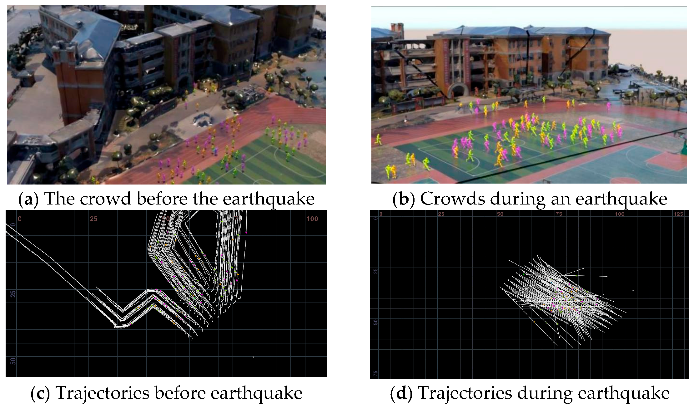
This scenario simulates a school environment during an earthquake, where individuals have already evacuated from buildings and are moving outdoors. We conducted simulations with 50, 100, and 500 agents. This experiment primarily validates the Variable-rotation Method and Local Routing Strategies One and Two (see Figure 20).

In the simulation experiment, this paper compares the scale of the scene, the authenticity of the scene, the size of the crowd and the calculation speed with reference [34], as shown in

Table 3. Comparisons of time costs during crowd simulation under different conditions.

Scene	Type and Condition	Size (Num)	Scene Scale and Realism	Time Costs (Seconds/Frame)
Crowd-1	Crowd, virtual Scene	8–148	simple, low	[0.001, 0.005]
Crowd-2	Crowd, virtual Scene	100	simple, low	[0.015, 0.029]
Traffic-1	Crowd/traffic, virtual Scene	30/35	medium, medium	[0.033, 0.038]
Traffic-2	People/bicycle/car, virtual Scene	25/15/40	medium, medium	[0.029, 0.034]
Ours	Crowd, real-scene 3D Variable-rotation Method with Strategies One and Two	50~500	complex, high	[0.026, 0.035]

. The results show that our method owns significant advantages in modeling scene. It demonstrates that the Variable-rotation Method and Local Routing Strategies One and Two are effective in various scenarios.

To further validate the effectiveness of our proposed methods, we compared our results with those of existing methods. Specifically, we compared our Variable-rotation Method (VRM) with the classic Social Force Model (SFM) [4], the Smoothed Particle Hydrodynamics Model (SPHM) [30] and the Cellular Automate Model (CAM) [35]. We conducted experiments in the same outdoor earthquake evacuation scenario, with the same number of agents (500 agents). The scene was reconstructed using the same oblique photography data to ensure consistency. Additionally, we also compared our methods with the Lattice Boltzmann Model (LBM) [35], which has been shown to be effective in predicting crowd dynamics (using the crowd dataset of UCF). These methods are widely used in behavior simulation of crowds and have been proven effective in various scenarios. The main evaluation indicators are Behavior Entropy (BE) [35] and Trajectory Bias Rate (TBR). The behavior entropy can describe the degree of chaos of velocity field, and the trajectory bias rate can evaluate the degree of deviation of path.

The Behavior Entropy (BE) of individual $\overrightarrow{\mathrm{X}}$ is as follows:

$${\mathrm{BE}}_{\overrightarrow{\mathrm{X}}}=-P_{\overrightarrow{\mathrm{X}}}{\log }_2{P}_{\overrightarrow{\mathrm{X}}}$$

(16)

$$P_{\overrightarrow{\mathrm{X}}}={\mathrm{e}}^{-1}+\eta (1-{\mathrm{e}}^{-1}),0\le \eta \le 1$$

(17)

$$\eta ={\displaystyle \frac{\left|{\displaystyle {\sum }_{\mathrm{i}=1}^{\mathrm{k}}{\overrightarrow{\mathrm{u}}}_i}\right|}{{\displaystyle {\sum }_{i=1}^k\left|{\overrightarrow{u}}_i\right|}}},\left|{\overrightarrow{u}}_i\right|\ne 0$$

(18)

where η denotes the velocity factor of other individuals in the vicinity of individual $\overrightarrow{\mathrm{X}}$, K represents the number of individuals within the domain, and U indicates the velocity.

Trajectory Bias Rate (TBR):

$$\mathrm{TBR}={\displaystyle \frac{{\displaystyle {\sum }_{\mathrm{i}=1}^k\left|Nod{e}_i(PathA)-Nod{e}_i(PathB)\right|}}{(Length(PathA)+Length(PathB))/2}}$$

(19)

Node_i(PathA) denotes the coordinates of the i-th node on the PathA, K represents the total number of nodes, and Length(PathA) indicates the path length. PathB is typically used as the reference path for evaluation.

The results show that several algorithms are good at simulating the movement of the crowd in the earthquake (outdoor), among which the algorithm of this paper has the best adaptability. This indicates that ours has obvious advantages in scene scale, scene authenticity, simulation effect, crowd resistance and repair force to the environment (

Table 4. Comparison of simulation results for different methods in the outdoor earthquake evacuation scenario.

Method	Dataset	Pathfinding Algorithm	TBR	BE
SFM [4]	Real scene 3D data	Shortest path	[0.5%, 5%], non-linear	[7500,8500], non-linear
SPHM [30]	Real scene 3D data	Minimal-rotation	[0.5%, 5%], non-linear	[7500,8500], non-linear
CAM [35]	Real scene 3D data	Shortest path	[0.5%, 5%], non-linear	[7500,8500], non-linear
LBM [35]	[Images in real life, UCF]	Shortest path	[0.5%, 5%], non-linear	[7250,8200], non-linear
This article	Real scene 3D data	Variable-rotation	[1%, 25%], non-linear	[7500,8500], non-linear

).

5.2. Indoor Earthquake Evacuation

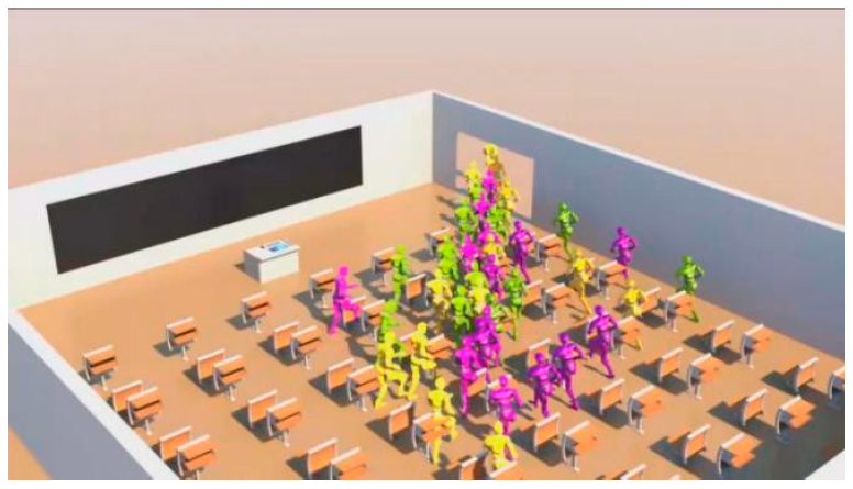
This scenario models evacuation from a building during an earthquake, accounting for falling objects, fusion computation of biological and solid-state types, and the application of the Spatial-Extrusion Method and Variable-Rotation Method. The experiment provides a visual comparison of these methods (see Figure 21 and Figure 22).

The experiment shows that the spatial-extrusion method works well when the external environment remains unchanged; however, when the external environment changes, the variable-rotation method is more appropriate.

Also, we compare our results with those of the Cellular Automate Model (CAM) [35], the Anisotropic Contractile Particle Model (ACPM) [25] and the Artificial Potential Field Model (APFM) [31]. The experiments are conducted in the indoor evacuation scenario, with the same number of agents (100 and 500).

As shown in

Table 5. Comparison of simulation results by different methods in the indoor earthquake evacuation scenario.

Method	Agents (Number)	Obstacles (Number)	Egress Time (Second)	External Condition	Emergent Behavioral Condition
CAM [35]	100	[1,2]	[10,25]	2D space, static environment, Shortest path	The evacuation time and density are negatively correlated (non-linear), and the steep slope inflection points exist at both ends of the evacuation relation curve.
CAM [35]	500	[1,2]	[25,30]
ACPM [25]	100	[1,2]	[10,25]		The evacuation time is negatively correlated (non-linear) with the number of static obstacles.
ACPM [25]	500	[1,2]	[25,30]
APFM [31]	100	500	[20,40]		The evacuation time is positively correlated with the number and width of exits (non-linear), and the steep slope inflection points exist at both ends of the evacuation relation curve.
APFM [31]	500	500	[80,120]
This article	100	100	[30,40]	3D space, dynamic environment. Variable-rotation, Spatial-extrusion, Strategy One to Two	There is a strong correlation between evacuation time and external emergencies. The variable-rotation method can effectively adapt to changes in the external environment.
This article	500	500	[110,200]

, that our method is more efficient, especially for large-scale simulations in uncertain environments.

5.3. Fish Crowd Activity

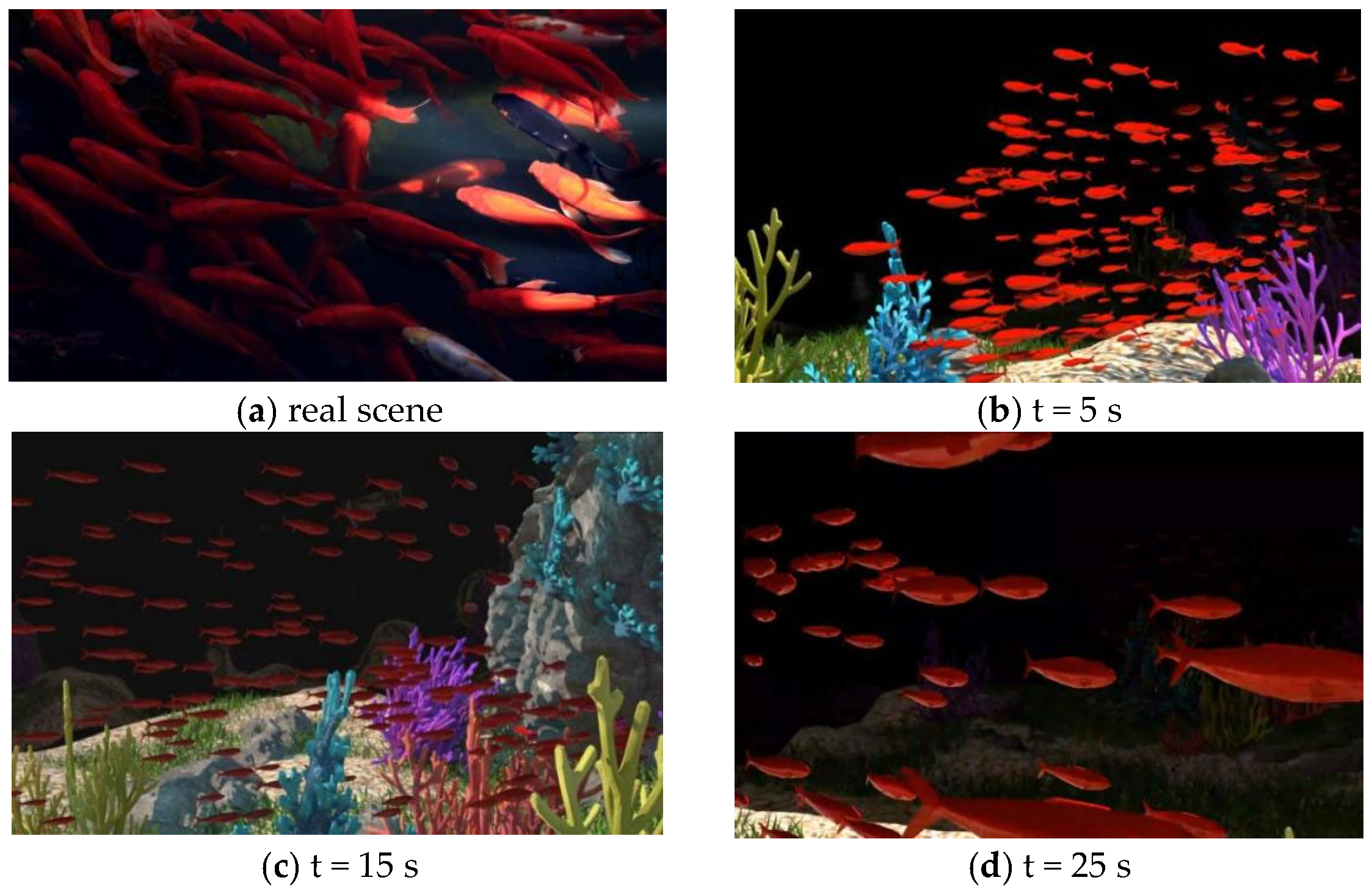
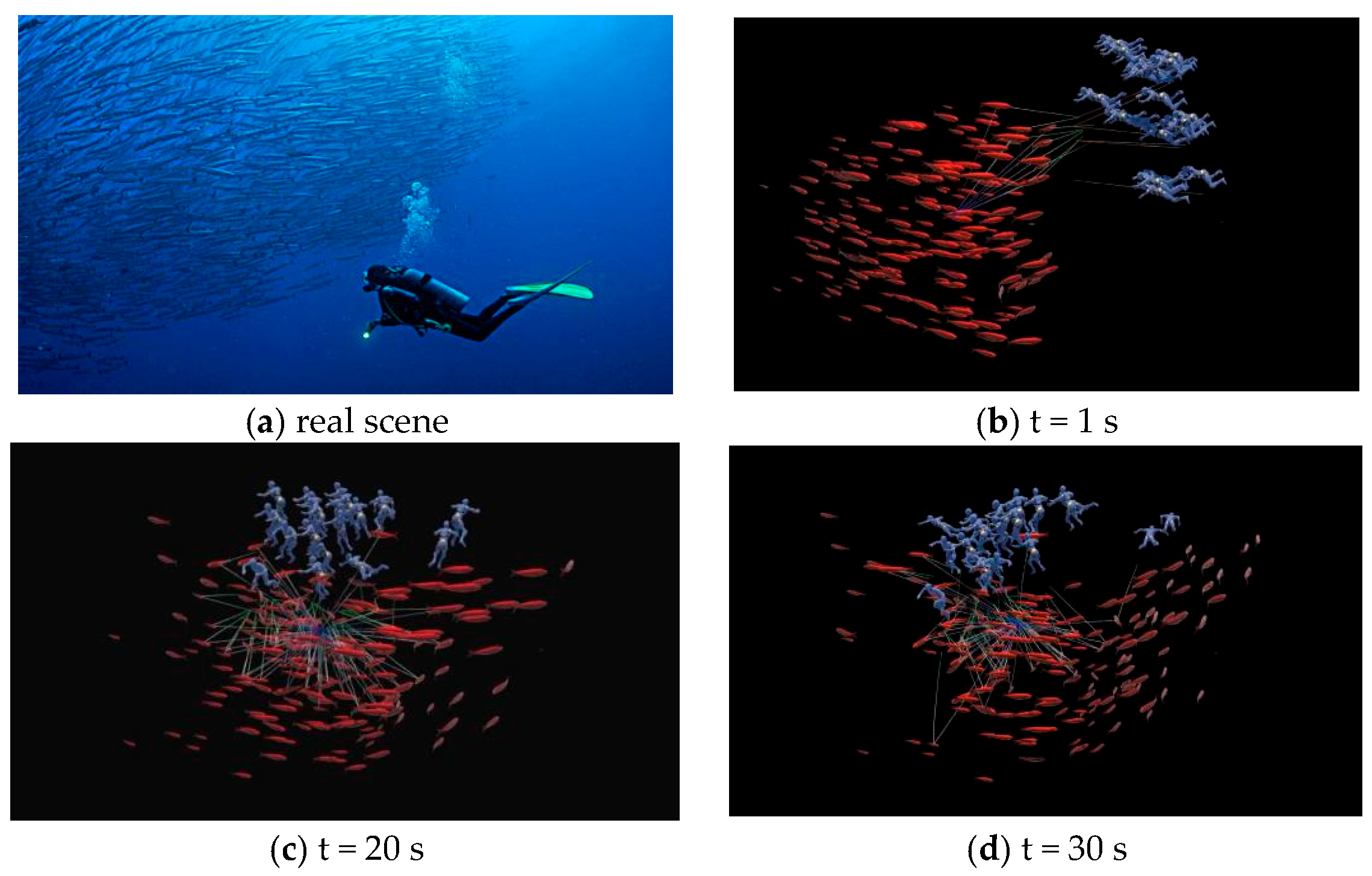
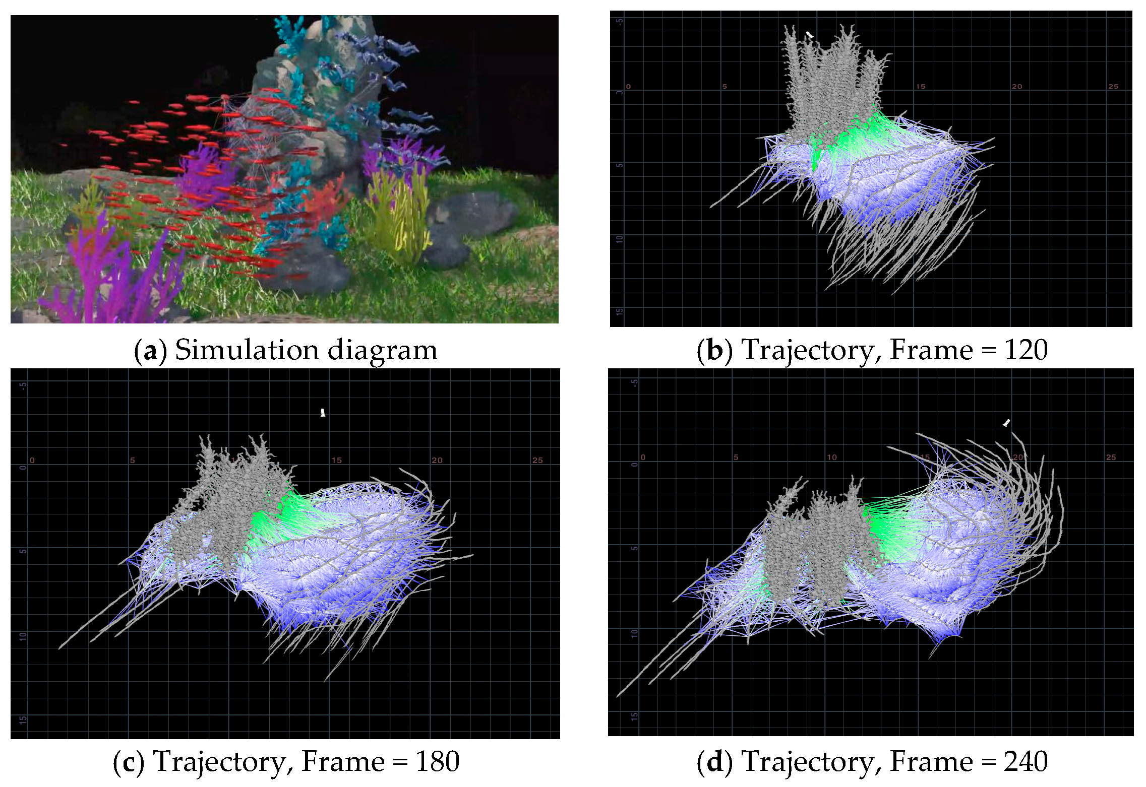
This experiment simulates fish migration and feeding behaviors in water, with simulation scales of 100 and 500 particles. The experiment validates Local Routing Strategy Three and Four, as shown in Figure 23 and Figure 24. In this experiment, the results of simulation are evaluated by comparing them with real-world images.

The experimental results show that in the process of fish simulation, this experiment has achieved a realistic simulation effect. At present, many scholars have used agent-based or mechanics-based methods to realize the large-scale biological cluster simulation of a single species. This paper adopts a hybrid model based on agent and mechanics. In terms of computational cost, simulation speed and scale, the method in this study has certain advantages and can be easily extended to biological clusters of multiple species.

Typically, we compare our results with recent work on the simulation of large-scale bird flocks using a Biologically Inspired Model (BIM) [34], which is based on Multi-agent approaches. The experiments are conducted in the same fish crowd activity scenario, with the same number of particles (100 and 500). The scene was reconstructed using the same data to ensure consistency.

Table 6. Comparison of simulation time for different methods in the fish crowd activity scenario.

Method	Number of Particles	Time Costs (Seconds/Frame)
BIM [34]	100	0.032
BIM [34]	500	0.038
This article: strategy three	100	0.025
This article: strategy three	500	0.028
This article: strategy four	100	0.029
This article: strategy four	500	0.032

indicates that our methods are more computationally efficient, especially for large-scale biological cluster simulations.

5.4. Underwater Fishing

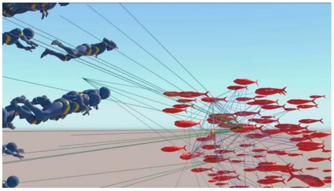
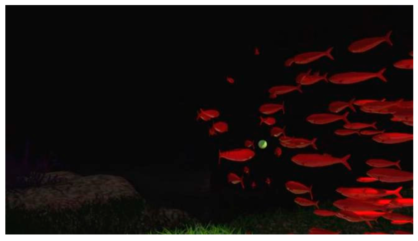
This simulation models the human pursuit of fish crowds underwater, involving the fusion computation of two biological types with 100 and 500 particles. The experiment validates Local Routing Strategy Five and Six (shown in Figure 25 and Figure 26).

This experiment mainly compares with real-world images to evaluate the simulation results. Experimental results confirm that both Strategies Five and Six produce realistic simulations. However, Strategy Six is computationally more efficient. The neighborhood nearest and neighborhood farthest selection mechanisms in Strategy Six sometimes lead to small subgroups being isolated.

To further demonstrate the effects of our strategies, we compare our results with the Boids Strategies and Steering Behaviors Strategies of Reynolds [3], which are agent-based models. The experiments were conducted in the same underwater fishing scenario, with the same number of particles (100 and 500). The scene was also reconstructed using the same data to ensure consistency.

Our method takes an average time of 0.032 s per frame for 500 particles, while reference [3] takes 0.042 s per frame. In terms of cluster strategy, this paper proposes a new innovative strategy: strategy six (neighborhood extreme value method). In terms of the driving model, this paper is based on the hybrid model of Agent-based and SPH, while the other two are based on an agent (

Table 7. Comparison of simulation results for different methods in the underwater fishing scenario.

Result Model Name	Reynolds’ Boids Strategies	Reynolds’ Steering Behaviors Strategies	The Equivalent Strategies of This Paper
Simulated emergent behaviors of clusters	Separation	Inherit Boids model	Strategy One, Two
	Alignment		Strategy Three
	Cohesion		Strategy Five
	/	Seek	Strategy Four
		Flee	Strategy Four
		Arrive	Strategy Three
		Wander	Strategy Three
		Pursuit/Evade	Strategy Four, Five
		Obstacle Avoidance	Strategy One, Two, Five
Does this mode support our Strategy Six?	No	No	Yes
Time cost (100 particles)	0.029	0.038	0.028
Time cost (500 particles)	0.033	0.042	0.032

).

5.5. Mine Field Landslide

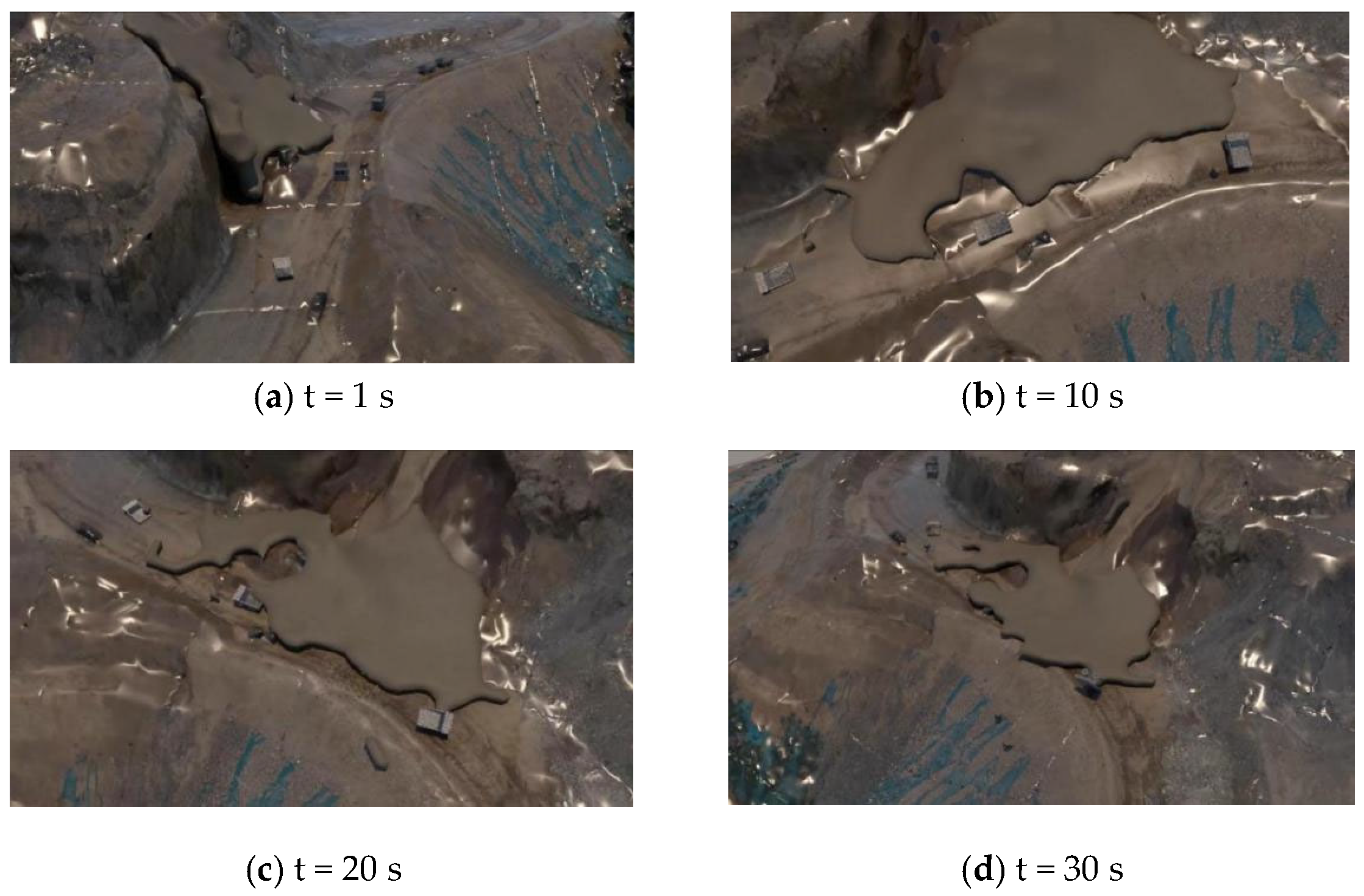
This experiment simulates a landslide occurring in a mining area during work hours, incorporating the fusion of two biological types and one solid-state type. The simulation was conducted with 100 and 500 particles and validated Local Routing Strategy Six (see Figure 27). In scenarios such as landslides and earthquakes, the computing objects in the neighborhood are roads or bunkers around individuals (the safe area that the crowd can reach).

In this simulation experiment, we compare the performance of the scene scale, the authenticity of the scene, the size of the crowd, the behavior entropy (BE), the trajectory bias rate (TBR) and the computing speed. The relevant data are shown in

Table 8. Time results under various conditions of mine field landslide scene.

Method	Particle Size	Scene Scale	Scene Realism	BE	TBR	Time Cost
MAS [15], Multi-agent and Shortest path	100	50,000 level	low	[0.5%, 5%], non-linear	[7500,8500], non-linear	0.033
	500	100,000 level	middle	[0.5%, 5%], non-linear	[7500,9000], non-linear	0.058
	500	150,000 level	high	[0.5%, 5%], non-linear	[000,10,7500], non-linear	0.092
This article, Multi-type particles fusion and Strategy six.	100	50,000 level	low	[1%, 25%], non-linear	[7500,8500], non-linear	0.021
	500	100,000 level	middle	[1%, 30%], non-linear	[7500,9000], non-linear	0.043
	500	150,000 level	high	[1%, 30%], non-linear	[000,10,7500], non-linear	0.087
Unit (particle size: number, scene scale: number of vertices, time cost: seconds/frame)

. To further demonstrate the effects of our method, we compare our results with the recent work on crowd simulation in natural disasters using a Multi-agent System (MAS, Shirvani et al. 2021, [15]). The experiments were conducted in the same mine field landslide scenario, with the same number of particles (100 to 500). The scene was also reconstructed using the same data to ensure consistency.

Experimental findings indicate that the integration of two biological types and one solid-state type is computationally feasible and yields high efficiency. The neighborhood nearest and neighborhood farthest approaches in Strategy Six are particularly suitable for such scenarios.

Our method takes an average simulation time of 0.043 s per frame for 500 particles, while Reference [15] takes 0.058 s per frame. This indicates that our method has higher computational efficiency, especially for large-scale simulations (Table 8).

6. Discussion

Compared with existing studies, we propose more generalized algorithms that can be applied across different special environment scenarios, by refining the fundamental principles of nature. Specifically, we focus on special natural phenomena such as earthquakes and landslides, refining an existing algorithm and introducing four new algorithms. Additionally, we explore fusion calculations for multi-type special interactions and investigate the application of agents across different species. These explorations establish a solid foundation for future work. By summarizing universal principles, our framework can be extended to other natural disasters, such as avalanches, volcanic eruptions, hurricanes, and insect infestations. This research provides a theoretical reference for future studies in the field.

The proposed model holds implications for early warning systems, disaster prediction, situation analysis, and scientific investigations, with the potential for diverse applications. Moving forward, we will conduct more in-depth experiments tailored to specific disaster scenarios and further investigate critical aspects, such as the driving mechanisms of agents, to enhance the depth of our research. Additionally, we aim to improve the computational efficiency and real-time performance of our algorithms to achieve greater practical applicability.

We intend to integrate our research across multiple disciplines by leveraging remote sensing images, oblique photography, and augmented reality. Through interdisciplinary collaboration, we aspire to contribute to the advancement of frontier research in this domain and explore innovative applications in disaster management and mitigation.

References

1. Dufour, O.; Dang, H.T.; Cordes, J.; Korbmacher, R.; Chraibi, M.; Gaudou, B.; Nicolas, A.; Tordeux, A. Dense Crowd Dynamics and Pedestrian Trajectories: A Multiscale Field Dataset from the Festival of Lights in Lyon. Sci. Data 2025, 12, 718. [Google Scholar] [CrossRef]
2. Ma, Y.; Liu, T.; Liu, Z. Diverse Motions and Responses in Crowd Simulation. Comput. Animat. Virtual Worlds 2024, 35, e70002. [Google Scholar] [CrossRef]
3. Reynolds, C.W. Steering behaviors for autonomous characters. In Proceedings of the Game Developers Conference, San Jose, CA, USA, 15–19 March 1999; Volume 1999, pp. 763–782. [Google Scholar]
4. Helbing, D.; Molnar, P. Social force model for pedestrian dynamics. Phys. Rev. E 1995, 51, 4282. [Google Scholar] [CrossRef] [PubMed]
5. Van den Berg, J.; Lin, M.; Manocha, D. Reciprocal velocity obstacles for real-time multi-agent navigation. In Proceedings of the 2008 IEEE International Conference on Robotics and Automation, Pasadena, CA, USA, 19–23 May 2008; IEEE: Piscataway, NJ, USA, 2008; pp. 1928–1935. [Google Scholar] [CrossRef]
6. Ondřej, J.; Pettré, J.; Olivier, A.H.; Donikian, S. A synthetic-vision based steering approach for crowd simulation. ACM Trans. Graph. (TOG) 2010, 29, 1–9. [Google Scholar] [CrossRef]
7. Hu, K.; Haworth, B.; Berseth, G.; Pavlovic, V.; Faloutsos, P.; Kapadia, M. Heterogeneous crowd simulation using parametric reinforcement learning. IEEE Trans. Vis. Comput. Graph. 2021, 29, 2036–2052. [Google Scholar] [CrossRef]
8. Funge, J.; Tu, X.; Terzopoulos, D. Cognitive modeling: Knowledge, reasoning and planning for intelligent characters. In Proceedings of the 26th Annual Conference on Computer Graphics and Interactive Techniques, Los Angeles, CA, USA, 8–13 August 1999; pp. 29–38. [Google Scholar] [CrossRef]
9. Shao, W.; Terzopoulos, D. Autonomous pedestrians. In Proceedings of the 2005 ACM SIGGRAPH/Eurographics Symposium on Computer Animation, Los Angeles, CA, USA, 29–31 July 2005; pp. 19–28. [Google Scholar] [CrossRef]
10. Patil, S.; Van Den Berg, J.; Curtis, S.; Lin, M.C.; Manocha, D. Directing crowd simulations using navigation fields. IEEE Trans. Vis. Comput. Graph. 2010, 17, 244–254. [Google Scholar] [CrossRef]
11. Loscos, C.; Marchal, D.; Meyer, A. Intuitive crowd behavior in dense urban environments using local laws. In Proceedings of the Theory and Practice of Computer Graphics, Birmingham, UK, 5 June 2003; IEEE: Piscataway, NJ, USA, 2003; pp. 122–129. [Google Scholar]
12. Best, A.; Narang, S.; Curtis, S.; Manocha, D. DenseSense: Interactive Crowd Simulation using Density-Dependent Filters. In Proceedings of the Symposium on Computer Animation, Copenhagen, Denmark, 21–23 July 2014; pp. 97–102. [Google Scholar] [CrossRef]
13. Heïgeas, L.; Luciani, A.; Thollot, J.; Castagné, N. A physically-based particle model of emergent crowd behaviors. arXiv 2010, arXiv:1005.4405. [Google Scholar] [CrossRef]
14. Golas, A.; Narain, R.; Lin, M. Hybrid long-range collision avoidance for crowd simulation. In Proceedings of the ACM SIGGRAPH Symposium on Interactive 3D Graphics and Games, Orlando, FL, USA, 21–23 March 2013; pp. 29–36. [Google Scholar] [CrossRef]
15. Shirvani, M.; Kesserwani, G.; Richmond, P. Agent-based simulator of dynamic flood-people interactions. J. Flood Risk Manag. 2021, 14, e12695. [Google Scholar] [CrossRef]
16. Shirvani, M.; Kesserwani, G.; Richmond, P. Agent-based modelling of pedestrian responses during flood emergency: Mobility behavioural rules and implications for flood risk analysis. J. Hydroinform. 2020, 22, 1078–1092. [Google Scholar] [CrossRef]
17. Clements, R.R.; Hughes, R.L. Mathematical modelling of a mediaeval battle: The battle of Agincourt, 1415. Math. Comput. Simul. 2004, 64, 259–269. [Google Scholar] [CrossRef]
18. Treuille, A.; Cooper, S.; Popović, Z. Continuum crowds. ACM Trans. Graph. (TOG) 2006, 25, 1160–1168. [Google Scholar] [CrossRef]
19. Narain, R.; Golas, A.; Curtis, S.; Lin, M.C. Aggregate dynamics for dense crowd simulation. In ACM SIGGRAPH Asia 2009 Papers; Association for Computing Machinery: New York, NY, USA, 2009; pp. 1–8. [Google Scholar] [CrossRef]
20. Chen, Q.; Luo, G.; Tong, Y.; Jin, X.; Deng, Z. A linear wave propagation-based simulation model for dense and polarized crowds. Comput. Animat. Virtual Worlds 2021, 32, e1977. [Google Scholar] [CrossRef]
21. van Toll, W.; Chatagnon, T.; Braga, C.; Solenthaler, B.; Pettré, J. SPH crowds: Agent-based crowd simulation up to extreme densities using fluid dynamics. Comput. Graph. 2021, 98, 306–321. [Google Scholar] [CrossRef]
22. Wei, L.; Freris, N.M. Multi-scale graph neural network for physics-informed fluid simulation. Vis. Comput. 2025, 41, 1171–1181. [Google Scholar] [CrossRef]
23. Nakamoto, H.; Takebayashi, H.; Fujita, M. Assessment of debris flow risk according to damage type. J. Disaster Sci. Manag. 2025, 1, 5. [Google Scholar] [CrossRef]
24. Takahashi, A.; Yasufuku, K. Evaluation of Tsunami Evacuation Plans for an Underground Mall Using an Agent-Based Model. J. Disaster Res. 2024, 19, 268–278. [Google Scholar] [CrossRef]
25. Nishino, K.; Ishida, T. Earthquake Virtual Reality Simulation System for Appropriate Evacuation Actions. In International Conference on P2P, Parallel, Grid, Cloud and Internet Computing; Springer Nature: Cham, Switzerland, 2024; pp. 292–301. [Google Scholar] [CrossRef]
26. Choi, Y.; Yang, S.; Kim, S. The smoke control system to improve the possibility of evacuation from fire disasters in high-rise buildings. Therm. Sci. Eng. Prog. 2025, 59, 103269. [Google Scholar] [CrossRef]
27. Borralho, T.M.O.; Rodrigues, J.P.C.; dos Santos, C.C. Evacuation of Lisbon’s Baixa-Chiado subway station in case of fire. Archit. Struct. Constr. 2025, 5, 11. [Google Scholar] [CrossRef]
28. Shukla, P.; Swami, K.; Gaddam, H.K. Simulation Based Passengers Emergency Evacuation Study for a Double Decker Train Coach. Transp. Res. Procedia 2025, 82, 1054–1070. [Google Scholar] [CrossRef]
29. Bernardini, G.; Cantatore, E.; Fatiguso, F.; Quagliarini, E. User Behaviour in Terrorist Acts to Model the Evacuation in Outdoor Open Areas. In Terrorist Risk in Urban Outdoor Built Environment: Measuring and Mitigating via Behavioural Design Approach; Springer Nature: Singapore, 2024; pp. 35–58. [Google Scholar] [CrossRef]
30. Zou, X.; Ye, Y.; Zhu, Z.; Chen, Q. Crowd evacuation simulation in flowing fluids. Comput. Animat. Virtual Worlds 2023, 34, e2161. [Google Scholar] [CrossRef]
31. Sha, Y. Research on Microscopic Simulation Model of Crowd Dispersion. Doctoral Dissertation, Tsinghua University, Beijing, China, 2008. [Google Scholar]
32. Demyen, D.; Buro, M. Efficient triangulation-based pathfinding. AAAI 2006, 6, 942–947. [Google Scholar] [CrossRef]
33. Xian, L. Human Dimensions of Chinese Adults Standard and Its Application. China Qual. Stand. Rev. 1994, 6, 2. [Google Scholar]
34. Ren, J. Multi-Agent System Simulation and Evaluation. Ph.D. Dissertation, Zhejiang University, Hangzhou, China, 2019. [Google Scholar]
35. Xue, Y. Study on the Model of Dense Population Flow and Evacuation Guidance Under Environmental Constraints. Ph.D. Dissertation, Harbin Institute of Technology, Harbin, China, 2023. [Google Scholar]
Figure 1. Crowds (biological clusters) in different natural environments.
Information 17 00049 g001
Figure 2. Comparison of three path planning methods. Reproduced with permission from Ref. [30]. Copyright 2023 Wiley.
Information 17 00049 g002
Figure 3. Schematic representation of traffic lane adjustments.
Information 17 00049 g003
Figure 4. Schematic diagram of the improved variable-rotation method. The variable-rotation method (green line) extends the minimal-rotation method [30] (red line) to allow customization.
Information 17 00049 g004
Figure 5. Local routing strategy one.
Information 17 00049 g005
Figure 6. Local routing strategy two.
Information 17 00049 g006
Figure 7. Local routing strategy three.
Information 17 00049 g007
Figure 8. Local routing strategy four.
Information 17 00049 g008
Figure 9. Local routing strategy five.
Information 17 00049 g009
Figure 10. Local routing strategy six.
Information 17 00049 g010
Figure 11. Schematic diagram of Spatial-extrusion method, part one.
Information 17 00049 g011
Figure 12. Schematic diagram of Spatial-extrusion method, part two.
Information 17 00049 g012
Figure 13. Simulation results of reference [31].
Information 17 00049 g013
Figure 14. Calculating flow of the simulator.
Information 17 00049 g014
Figure 15. UAV data acquisition process.
Information 17 00049 g015
Figure 16. Scene importing.
Information 17 00049 g016
Figure 17. Results of feature separation.
Information 17 00049 g017
Figure 18. Low-resolution mesh generation.
Information 17 00049 g018
Figure 19. Integration computation of biological type and solid-state type.
Information 17 00049 g019
Figure 20. Schematic diagram of outdoor earthquake evacuation.
Information 17 00049 g020
Figure 21. Indoor escape (Spatial-extrusion method).
Information 17 00049 g021
Figure 22. Indoor escape (Variable-rotation method).
Information 17 00049 g022
Figure 23. Verifying local routing strategy three.
Information 17 00049 g023
Figure 24. Verifying local routing strategy four.
Information 17 00049 g024
Figure 25. Verifying the local routing strategy five (crowd center method).
Information 17 00049 g025
Figure 26. Verifying the local routing strategy six (neighborhood extreme value method).
Information 17 00049 g026
Figure 27. Verifying the computation of multi-type particle fusion and strategy six.
Information 17 00049 g027