On Measuring Large Language Models Performance with Inferential Statistics

Abstract

Measuring the reliability of performance evaluations is particularly important when we evaluate non-deterministic models. This is the case of using large language models (LLMs) in classification tasks, where different runs generate different outputs. This fact raises the question about how reliable the evaluation of a solution is. Previous work relies on executing several runs and then taking some kind of average together with confidence intervals. However, confidence intervals themselves may not be reliable if the number of executions is not large enough. Therefore, more effective and robust methods are needed for their estimation. In this work, we propose a methodology that estimates model performance while capturing the intra-run variability by leveraging instance-level predictions across multiple runs, enabling the computation of more reliable confidence intervals when the gold standard is available. Our method also offers greater computational efficiency by reducing the number of full model executions required to estimate performance variability. Compared against existing state-of-the-art evaluation methods, our approach achieves full empirical coverage (100%) of plausible performance outcomes using as few as three runs, whereas traditional methods reach at most 63% coverage, even with eight runs.

1. Introduction

When addressing a problem through machine learning, practitioners frequently employ non-deterministic models or those whose outputs depend on parameters that are difficult to control, such as pseudo-random number generation. In particular, with the emergence of LLMs in natural language processing (NLP), a variety of architectures and strategies have been proposed to tackle specific tasks. However, as demonstrated in [1,2,3], these LLMs produce different text outputs even under the most deterministic parameter configurations, with observed accuracy deviations of up to 15%.

Despite awareness of this phenomenon, many studies—often constrained by the computational cost of repeated runs—report only a single execution result for their algorithms, rendering comparisons difficult and reproducibility poor. This approach is common in benchmark evaluations of LLMs, where performance is typically reported as a single number [4,5,6,7].

To address these limitations, several inferential statistical methodologies have been developed for model and algorithm comparison. A taxonomy of statistical questions in machine learning, focusing on how to decide whether one of two algorithms yields better classifiers on a dataset, was introduced in [8]. He recommended the $5\times 2$ cv t-test or McNemar’s test [9] on the misclassification matrix when multiple runs are infeasible. Later, Bouckaert [10,11] investigated experimental replicability in machine learning, proposing the use of a resampled t-test instead of the $5\times 2$ cv t-test.

Moreover, with large sample sizes, even small differences can achieve statistical significance, prompting researchers in many fields to recommend reporting effect size measures to contextualize the practical importance of results [12,13,14,15]. Another strategy is to report confidence intervals for performance metrics, which provide a range of plausible values for the true performance [16]. This latter study uses instance-level predictions from both models rather than relying on a single aggregated performance value to obtain the difference in performance between them. While [16] also employs instance-level bootstrapping, it specifically focuses on comparing two models with numerical outputs using the estimator of the difference in performance for each prediction. Ref. [17] compared the advantages and disadvantages of hypothesis tests versus confidence intervals for classifier comparison, concluding that confidence intervals offer a slight advantage.

Rather than comparing multiple systems, Soboroff [18] proposed using bootstrap techniques to study the performance distribution of a single classifier on multi-topic classification problems. By executing the same algorithm many times, one obtains a distribution of the metric of interest per topic, from which topic-specific confidence intervals can be computed. In addition to bootstrapping, the paper also applies the Central Limit Theorem [19], approximating the distribution of the sample mean using a Student’s t-distribution to construct confidence intervals when the number of runs is limited.

Our work adopts this latter approach: we focus on assessing the performance of a single system in scenarios where each run incurs a high computational cost. While previous studies aim to estimate the system’s average performance using aggregated evaluation metrics from each run, our approach introduces an evaluation methodology that leverages the labels of individual instances rather than aggregated scores to capture the inherent variability across runs. This allows us to construct confidence intervals that more realistically reflect the range of possible predictions, providing a more accurate and informative assessment of model performance. Moreover, our method is computationally efficient, minimizing the number of costly runs needed to obtain reliable estimates.

The remainder of this paper is organized as follows. In the rest of the introduction, we delineate our objectives, contributions, and research questions. Section 2 defines the experimental setup, including the dataset and evaluation metric. Section 3 presents our evaluation methodology for settings where full test-set labels are available. We then demonstrate an empirical application of our approach and compare it against state-of-the-art evaluation methods. Finally, we conclude with a discussion of its limitations and potential directions for future research.

1.1. Objectives

The main objective of this work is to establish a statistically sound methodology for reliably evaluating the performance of large language models (LLMs) in classification tasks. Given the non-deterministic nature of these models, we focus on the scenario where the full set of test labels is available. Our goal is to ensure that performance estimates accurately reflect the model’s actual capabilities by accounting for the inherent variability across different runs.

In order to achieve the proposed general objective, a series of specific objectives are set out below to guide the methodological development of the work.

• Develop a robust and efficient evaluation framework capable of withstanding the variability introduced by non-deterministic models.
• Establish confidence intervals for performance metrics in the evaluation scenario where access to individual outputs and gold standard labels is available.
• Provide empirical evidence demonstrating the variability across multiple runs of a non-deterministic model and illustrate how the use of the proposed evaluation system can lead to more reliable and informative performance assessments.

1.2. Contributions

This study provides the following key contributions to the robust evaluation of non-deterministic models, in particular LLMs, in classification tasks:

• Statistical analysis of evaluation variability: We provide empirical evidence showing that performance metrics obtained from single runs can vary significantly, highlighting the need for repeated evaluations to obtain reliable performance estimates.
• Confidence interval estimation: We propose a methodology for calculating confidence intervals for performance metrics. This method allows the uncertainty associated with model evaluation to be quantified.
• Model-independent assessment framework: The proposed methodology is designed to be robust to different model architectures and prompts.

In conclusion, these contributions provide a practical and statistically supported methodology to improve the reliability and reproducibility of LLM evaluations.

1.3. Research Questions

In this study, we aim to answer two main research questions that apply to both evaluation environments.

RQ1.

Is a single run enough to evaluate the performance of a generative model, and do the results of multiple runs vary in a statistically significant way?

RQ2.

Can we estimate the true performance of a given approach by aggregating multiple runs with identical configurations?

RQ3.

Which statistical techniques provide the most reliable and efficient approximation of model performance variability in non-deterministic settings?

These questions aim to measure the reliability and statistical robustness of evaluation procedures applied to non-deterministic models and to quantify the uncertainty associated with single-run evaluations.

2. Experimentation Setting

This section describes the key elements that make up the experimental setting of the study. First, the dataset used for the classification task is detailed, including its main characteristics and the evaluation criteria used. Next, the language models used are presented, as well as the different prompting configurations and parameters applied during generation.

2.1. Dataset

In this study, we use the dataset developed within the framework of the paper [20]. This dataset focuses on the creation of a dataset for automatic narrative identification in the political domain and has been used in the DIPROMATS 2024 shared task.

The dataset comprises two narrative identification tasks in the political domain, developed in both Spanish and English. Each task includes tweets published by diplomats from different regions (China, Russia, European Union, and United States of America), annotated to reflect the presence of specific narratives. Each region has been assigned six narratives, and for each language, there are 800 manually annotated tweets.

For each tweet and each narrative, there are three possible labels. In this dataset, the annotation scheme follows a ternary annotation, binary classification framework (A3C2). Annotators can assign one of three possible labels to each tweet with respect to a given narrative: yes, no, or leaning. The leaning label was introduced to capture instances where the support for a narrative was subtle, implicit, or open to interpretation.

In our study, we focus exclusively on the subset of Spanish tweets. The distribution of the labels for this dataset can be seen in

Table 1. Distribution of labels by narrative and region in the test set for the Spanish language.

Region/Nar.	Yes	Leaning	No	Region/Nar.	Yes	Leaning	No
CH1	21	8	171	RU1	34	12	154
CH2	65	9	126	RU2	4	15	181
CH3	6	0	194	RU3	30	28	142
CH4	24	24	152	RU4	25	19	156
CH5	12	21	167	RU5	22	25	153
CH6	22	11	167	RU6	14	10	176
China	150	73	977	Russia	129	109	962
EU1	14	10	176	US1	23	1	175
EU2	29	21	150	US2	19	5	175
EU3	24	23	153	US3	46	11	142
EU4	31	23	146	US4	66	23	110
EU5	79	33	88	US5	37	18	144
EU6	48	65	87	US6	11	4	184
European Union	225	175	800	USA	202	62	930

.

2.2. Evaluation Measure

For annotation purposes, the DIPROMATS dataset has an additional label named leaning to address the subjectivity inherent in the narrative classification task. As a result, three different evaluation metrics were used depending on the consideration of the leaning cases [20]: F1-strict, F1-lenient and F1-average.

In this study, we will use only the F1-strict (from now on, F1) metric for performance evaluation, although the methodology and results are generalizable to any other evaluation metric. F1-strict will be calculated from the precision and recall over the class yes for each narrative. In other words, the leaning cases in the gold standard will be considered as the class no.

3. Methodology

The steps of the methodology are the following (described in each subsection): (i) generation of runs; (ii) approximation of the theoretical distribution of model performance; (iii) confidence interval estimation; and (iv) analysis of aggregated F1 means.

3.1. Performing Multiple Executions

Even after fixing the dataset and the LLMs used for the study, the variability among predictions remains significant. To measure this variability, the first step is the generation of several runs over the same dataset and model with a fixed configuration.

3.2. Approximation of the Theoretical Distribution of Model Performance

Given a set of n independent runs of the same model with identical parameters and prompting strategy, and assuming the existence of a gold standard of size l with known true labels, it is possible to approximate the theoretical distribution of model performance for each run using a uniform bootstrapping approach [21]. (This bootstrap approach was selected to illustrate the methodology in a clear and general way, prioritizing interpretability over dataset-specific optimisations.)

The procedure is as follows:

• Let $\mathcal{D}=\{(x_1,y_1),\dots ,(x_l,y_l)\}$ be the set of predicted labels $x_i$ and their corresponding true labels $y_i$ for run r, where l is the number of instances in the test set. The sample size l should be sufficiently large to obtain meaningful performance distributions. (A sufficiently large sample size reduces variability and ensures stable F1 estimates. Empirically, at least 30–50 examples per class are recommended, with larger sets (>300–1000) needed for reliable distributions and >5000 for complex or industrial settings. Small samples yield unstable, high-variance, or biased estimates.)
• Generate B bootstrap samples with replacement from the original set $\mathcal{D}$, obtaining B new datasets ${\mathcal{D}}_b^{\ast }$ ($b=1,\dots ,B$), each of size l. Each ${\mathcal{D}}_b^{\ast }$ contains a resampled set of predicted–true label pairs.
• For each bootstrap sample ${\mathcal{D}}_b^{\ast }$, compute the F1 score, denoted $F{1}_b^{\ast }$. This represents the model’s performance on the b-th resampled dataset.
• The set of bootstrap F1 scores $\{F{1}_1^{\ast },F{1}_2^{\ast },\dots ,F{1}_B^{\ast }\}$ defines the empirical distribution of model performance for run r, which we denote as $\mathcal{F}{1}_r$.
• Estimate the theoretical F1 value for run r as the mean of the bootstrap scores:

  $${\widehat{F1}}_r={\displaystyle \frac{1}{B}}\sum _{b=1}^{B}F{1}_b^{\ast },$$

  (1)

  where ${\widehat{F1}}_r$ provides a point estimate of the model’s expected F1 for this run.

By repeating this process for all n runs, we obtain n approximated distributions of the model’s performance. By using resampling with replacement, we account for the diversity and variability in the predictions of each run. The randomness introduced by replacement allows misclassified instances to be repeated across samples, effectively simulating the presence of similar challenging instances in a hypothetical future dataset. To assess whether these distributions differ significantly in their central tendency, statistical tests can be applied: a t-test for normally distributed data, or a Mann–Whitney U test when normality cannot be assumed.

If significant differences are detected among runs, a more robust approximation of the true performance distribution can be obtained by concatenating the prediction–label pairs from multiple runs into a single dataset of size $l\times m$, where m is the number of runs to be concatenated, and applying the same bootstrapping procedure. This strategy increases the diversity of the data and reduces the estimation bias of individual runs.

As the number of combined runs increases, the number of significant differences between the distributions generated from 1, 2, …, n combined runs is expected to decrease, indicating that the approximation is converging toward the true performance distribution of the model.

The mean F1 score obtained from the distribution built using all available runs, ${\widehat{F1}}_{1,\dots ,n}$, is considered the most accurate approximation of the model’s true performance.

On the other hand, if no statistically significant differences are found among the distributions from individual runs, any of them may be considered a sufficiently accurate approximation of the model’s true performance.

3.3. Analysis of Aggregated F1 Means

Let $F{1}_r$ be the aggregated F1 score obtained from a single run r, and let ${\widehat{F1}}_{1,\dots ,n}$ be the corresponding estimated theoretical value obtained via bootstrapping using n runs. Empirically, we observe that there exists a consistent deviation between $F{1}_r$ and ${\widehat{F1}}_{1,\dots ,n}$:

$$F{1}_r\ne {\widehat{F1}}_{1,\dots ,n}$$

(2)

indicating that a single run’s aggregated F1 score may not be a reliable estimate of the model’s true performance.

Now consider a subset of m runs $S=\{i_1,\dots ,i_m\}$. Let the average aggregated F1 across these runs be

$${\overline{F1}}_S={\displaystyle \frac{1}{m}}\sum _{j=1}^{m}F{1}_{i_j}$$

(3)

As m increases, this average tends to converge to the expected theoretical value obtained from the combined distribution of those m runs, ${\widehat{F1}}_{i_1,\dots ,i_m}$, and further to the global theoretical estimate obtained from all n available runs, ${\widehat{F1}}_{1,\dots ,n}$:

This property supports the idea that the average aggregated F1 score over multiple runs serves as a consistent estimator of the model’s true expected performance. Moreover, this estimation can be obtained without requiring full access to test labels or the computation of bootstrap-based distributions, which are otherwise necessary to estimate ${\widehat{F1}}_{1,\dots ,n}$.

This assumption holds when n is sufficiently large, ensuring that the empirical mean reliably approximates the true expected value. However, in scenarios where the number of runs n is limited, relying solely on the aggregated F1 mean might be misleading. In such cases, providing a confidence interval for the estimated F1 score becomes crucial, as it offers a more robust and informative assessment of the model’s expected performance.

3.4. Confidence Interval Estimation

Given a distribution $\mathcal{F}{1}_r=\{F{1}_1^{\ast },F{1}_2^{\ast },\dots ,F{1}_B^{\ast }\}$ of B bootstrap estimates for a run r, the $(1-\alpha )·100\%$ confidence interval can be computed non-parametrically using the percentile method [22] as follows:

• The B bootstrap values $F{1}_b^{\ast }$ are sorted in ascending order to approximate the empirical distribution of $F1$.
• The confidence interval at level $(1-\alpha )$ is defined by the ${\displaystyle \frac{\alpha }{2}}$ and $1-{\displaystyle \frac{\alpha }{2}}$ percentiles of the ordered bootstrap distribution:

  $$CI=\left[F{1}_{({\displaystyle \frac{\alpha }{2}}·B)}^{\ast },F{1}_{((1-{\displaystyle \frac{\alpha }{2}})·B)}^{\ast }\right]$$

  (4)

  where $F{1}_{\left(j\right)}^{\ast }$ denotes the j-th smallest value among the B estimates.

This confidence interval provides a quantification of the variability in the model’s performance estimate. In the worst-case scenario—assuming runs are ordered from lowest to highest aggregate F1—the confidence interval helps establish a range within which the F1 scores of future runs are expected to lie with high probability. This interval thus offers a statistical guarantee about the model’s stability and reliability under repeated evaluation.

3.5. Proposed Evaluation Framework

Building upon the mathematical foundations described in the previous sections, we propose a bootstrapping-based evaluation framework at the instance level. To robustly estimate the performance of a model across multiple independent runs, all available predictions from the n runs are concatenated with the corresponding true labels to form a single aggregated dataset of size $l\times n$, where l is the number of instances in the gold standard.

From this aggregated dataset, an empirical distribution of F1 scores is generated by repeatedly sampling instance-level prediction–label pairs with replacement. Each bootstrap sample is used to compute an F1 score, capturing potential fluctuations in performance that could occur on similar datasets. The mean of the resulting bootstrap distribution, ${\widehat{F1}}_{1,\dots ,n}$, provides a robust estimate of the model’s expected performance.

Finally, a $(1-\alpha )·100\%$ confidence interval is computed using the percentile method applied to the bootstrap distribution, quantifying the uncertainty around the estimated mean performance.

Algorithm 1 summarizes this procedure, illustrating the construction of the empirical performance distribution and the corresponding confidence interval.

Algorithm 1 Instance-Level Bootstrapping Evaluation Framework

Require: Predictions from n runs, gold standard of size l, number of bootstrap samples B, confidence level $(1-\alpha )$ Ensure: Combined distribution $\mathcal{F}{1}_{1,\dots ,n}$, mean estimate ${\widehat{F1}}_{1,\dots ,n}$, confidence interval $CI$     Concatenate predictions from all n runs into dataset ${\mathcal{D}}_{1,\dots ,n}$ of size $l\times n$     for $b=1,\dots ,B$ do         Sample l pairs with replacement from ${\mathcal{D}}_{1,\dots ,n}\to {\mathcal{D}}_b^{\ast }$         Compute $F{1}_b^{\ast }$ on ${\mathcal{D}}_b^{\ast }$     end for     Define empirical distribution $\mathcal{F}{1}_{1,\dots ,n}=\{F{1}_1^{\ast },\dots ,F{1}_B^{\ast }\}$     Estimate mean performance: $${\widehat{F1}}_{1,\dots ,n}={\displaystyle \frac{1}{B}}\sum _{b=1}^{B}F{1}_b^{\ast }$$     Sort $\{F{1}_1^{\ast },\dots ,F{1}_B^{\ast }\}$ in ascending order     Define confidence interval: $$CI=\left[F{1}_{(\alpha /2·B)}^{\ast },F{1}_{\left(\right(1-\alpha /2)·B)}^{\ast }\right]$$

4. Running Example

In this section, we illustrate the application of the methodology presented Section 3. The procedures are applied using the experimentation settings previously defined in Section 2.

4.1. Performing Multiple Executions

In this study, the Qwen2.5-3B-Instruct model [23] is used to address the classification task. The model was run 30 independent times to analyze its performance stability and the convergence of the error as the number of runs increases. This model was evaluated using a zero-shot prompting strategy with the same prompt consistently across all runs. To maintain experimental consistency, the model was run with a temperature of 0.75 and a top-k value of 5 during response generation. The prompt used can be found in Appendix A, with modifications adapted to each specific country.

4.2. Approximation of the Theoretical Distribution of Model Performance

As previously described, bootstrap-based distributions have been generated for each run and for all possible combinations of runs for every evaluated approach. The resampling process uses $B=5000$ bootstrap replicates to approximate the underlying performance distribution.

To illustrate this, Figure 1 shows the bootstrap distributions corresponding to Runs 1 through 5, as well as the aggregated distribution combining all five runs of the Qwen 3B zero-shot approach. These distributions serve as empirical approximations of the model’s performance and reveal the reduction in variability as more runs are incorporated.

Moreover, we studied how increasing the number of aggregated runs affects statistical consistency. Our analysis shows that as the number of accumulated runs grows, the percentage of statistically significant differences between the estimated means of different run combinations decreases. For example, when considering aggregated results over one, two, three, and four runs respectively, the proportion of run combinations showing significant differences was approximately 96, 89, 82, and 70%. This effect is primarily due to the reduction in the standard error of the estimated mean as more runs are aggregated, rather than a true decrease in the underlying run-to-run variability. Aggregating more runs therefore stabilizes the performance estimates by reducing the uncertainty of the estimator, lowering the likelihood of detecting significant differences that arise purely by chance.

4.3. Analysis of Aggregated F1 Means

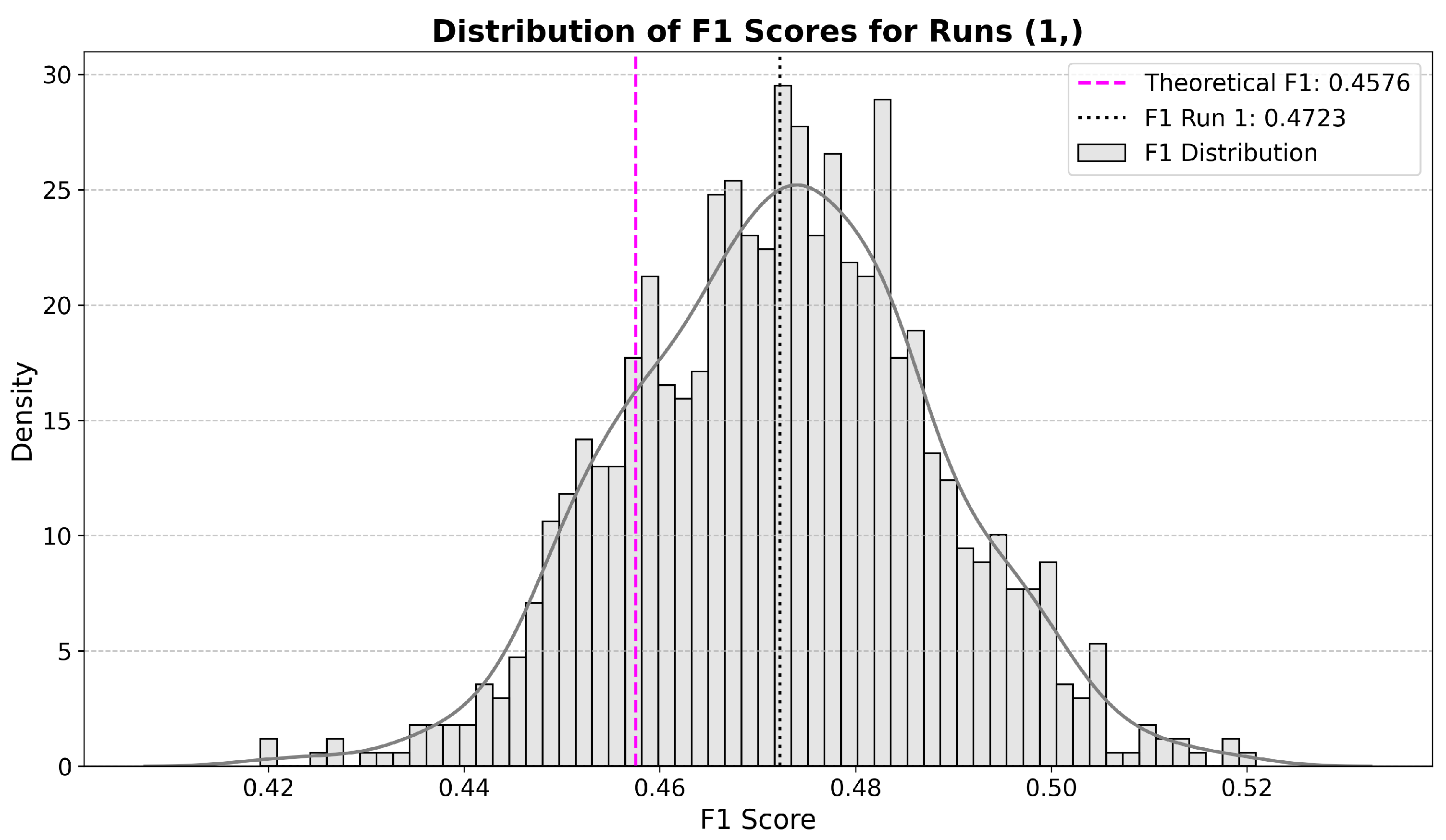
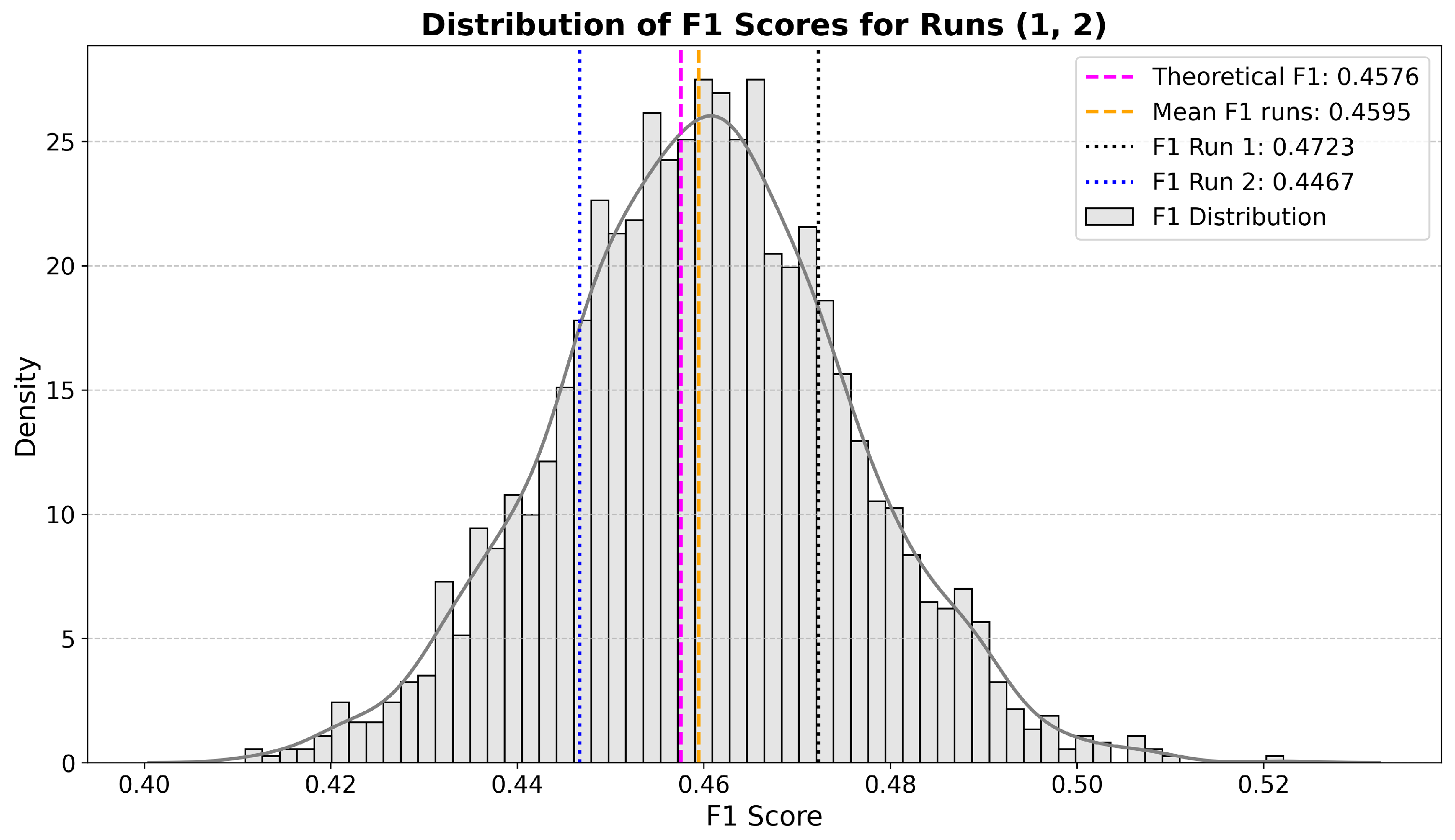
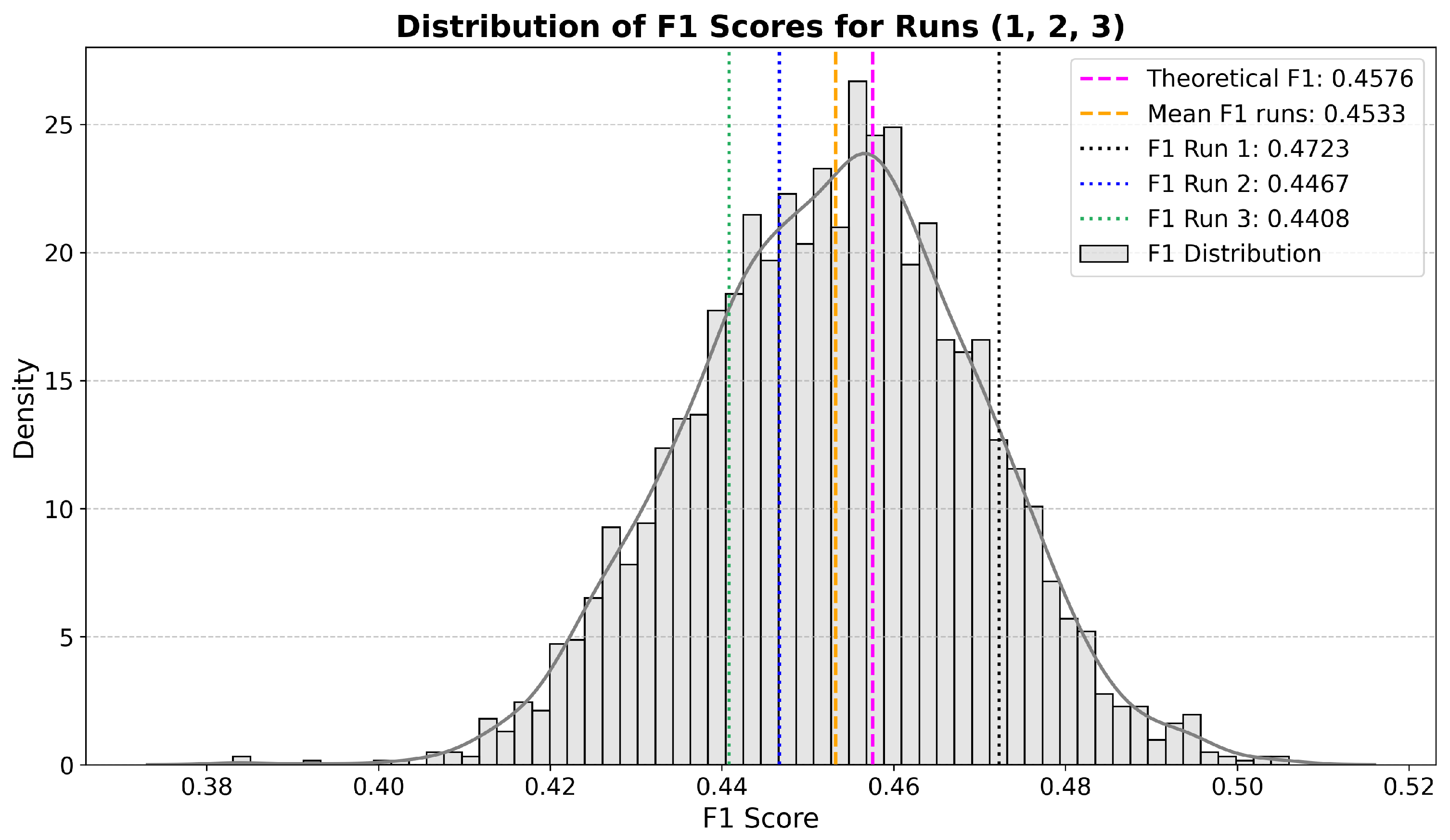
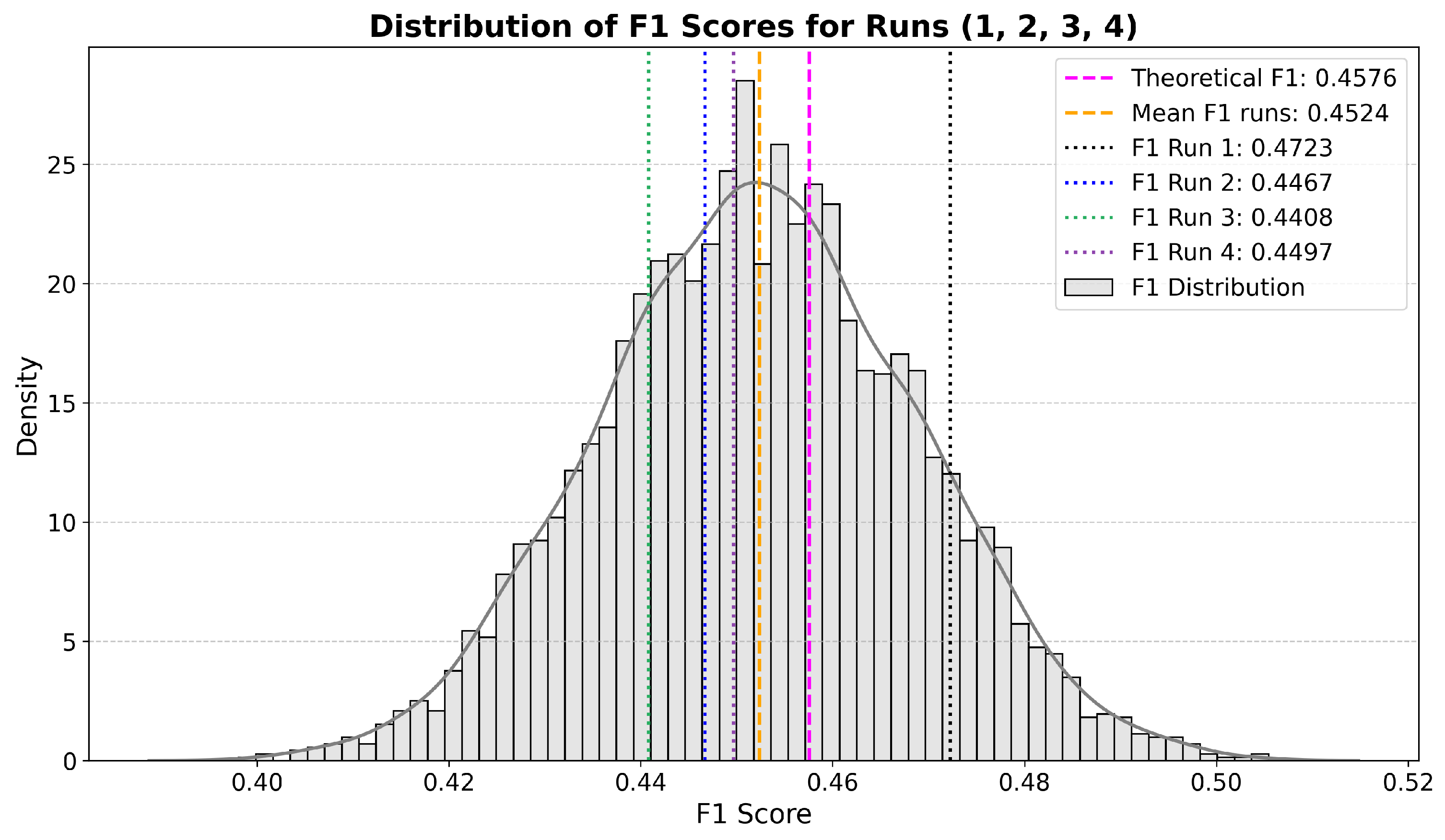
As previously discussed, we have analyzed the comparison between the aggregated F1 means and the theoretically estimated F1 value, ${\widehat{F1}}_{1,\dots ,5}$. To illustrate, the cumulative distributions for the Qwen 3B Z-S approach are presented in Figure 2, Figure 3, Figure 4 and Figure 5, along with the aggregated F1 values for each run, the mean of these aggregated values, and the theoretical F1 estimate.

It is important to note that convergence between the aggregated F1 means and ${\widehat{F1}}_{1,\dots ,5}$, is not guaranteed when the number of available n runs is small—as in this case, with only five runs—which limits the reliability of this approach. In fact, the relative error does not systematically decrease as more runs are added.

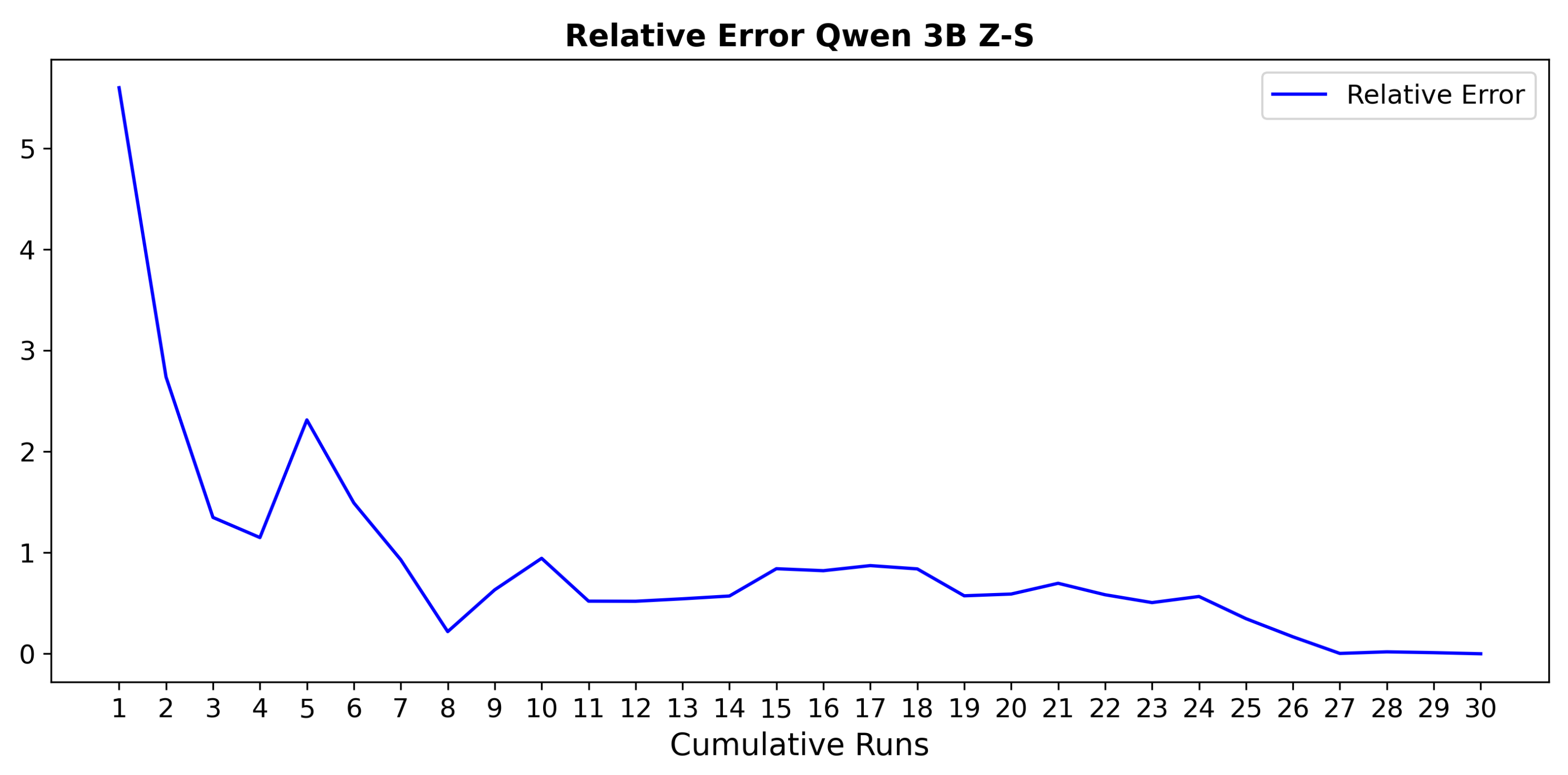
To further examine this behavior under a more comprehensive experimental setup, we analyze the convergence trend using a larger number of runs. As shown in Figure 6, the relative error between the aggregate mean and the theoretical value clearly decreases as more runs are included, corroborating the hypothesis that, with a sufficiently large number of runs, the aggregate mean becomes a consistent estimator of the true model performance.

4.4. Confidence Interval Estimation

As previously described, the $95\%$ confidence intervals are computed using the percentile method.

Table 2. Confidence intervals at $95\%$ computed for cumulative combinations of the first five runs of the Qwen 3B zero-shot approach in scenario 1.

Runs	CI	$\mathbf{\Delta }$CI
(1)	(0.4424, 0.5027)	0.0602
(1, 2)	(0.4292, 0.4905)	0.0613
$(1,\dots ,3)$	(0.4211, 0.4841)	0.0630
$(1,\dots ,4)$	(0.4203, 0.4838)	0.0634
$(1,\dots ,5)$	(0.4255, 0.4889)	0.0634

reports the confidence intervals for the first five runs of the model, calculated over cumulative combinations of runs: first using only Run 1, then Runs 1 and 2, and so on up to the full combination of Runs 1 through 5. It can be observed that, as more runs are aggregated, the resulting confidence intervals tend to stabilize and converge toward the interval obtained from all five runs.

However, this convergence could be disrupted in the worst-case scenario where, due to randomness, the runs are ordered from the lowest to the highest aggregated F1 score (or vice versa). It is important to note that such an arrangement of runs is extremely unlikely to occur in practice, but it serves to illustrate the limits of the proposed methodology under the most unfavorable conditions. In this situation, we would not observe stabilization until all runs have been included. To simulate this adverse scenario, we ordered the runs by increasing aggregated $F1$ score $(a_1,\dots ,a_{30})$ and studied whether the aggregated $F1$ scores of the remaining, non-included runs fall within the $95\%$ confidence interval derived from the cumulative subset. This analysis is shown in

Table 3. Worst-case evaluation of whether individual run F1 scores fall within the $95\%$ confidence intervals computed from incremental combinations for the 30 Qwen 3B Z-S runs.

	Sorted Runs
	${\mathit{a}}_{\mathbf{2}}$	…	${\mathit{a}}_{\mathbf{24}}$	${\mathit{a}}_{\mathbf{25}}$	${\mathit{a}}_{\mathbf{26}}$	${\mathit{a}}_{\mathbf{27}}$	${\mathit{a}}_{\mathbf{28}}$	${\mathit{a}}_{\mathbf{29}}$	${\mathit{a}}_{\mathbf{30}}$
$\left(a_1\right)$	✓	✓	✓	✗	✗	✗	✗	✗	✗
$(a_1,a_2)$	-	✓	✓	✗	✗	✗	✗	✗	✗
$(a_1,\dots ,a_3)$	-	✓	✓	✗	✗	✗	✗	✗	✗
$⋮$	-	✓	✓	✗	✗	✗	✗	✗	✗
$(a_1,\dots ,a_7)$	-	✓	✓	✗	✗	✗	✗	✗	✗
$(a_1,\dots ,a_8)$	-	✓	✓	✓	✗	✗	✗	✗	✗
$⋮$	-	✓	✓	✓	✗	✗	✗	✗	✗
$(a_1,\dots ,a_{11})$	-	✓	✓	✓	✗	✗	✗	✗	✗
$(a_1,\dots ,a_{12})$	-	✓	✓	✓	✓	✓	✗	✗	✗
$⋮$	-	✓	✓	✓	✓	✓	✗	✗	✗
$(a_1,\dots ,a_{15})$	-	✓	✓	✓	✓	✓	✗	✗	✗
$(a_1,\dots ,a_{16})$	-	✓	✓	✓	✓	✓	✓	✗	✗
$⋮$	-	✓	✓	✓	✓	✓	✓	✗	✗
$(a_1,\dots ,a_{19})$	-	✓	✓	✓	✓	✓	✓	✗	✗
$(a_1,\dots ,a_{20})$	-	✓	✓	✓	✓	✓	✓	✓	✗
$⋮$	-	✓	✓	✓	✓	✓	✓	✓	✗
$(a_1,\dots ,a_{28})$	-	-	-	-	-	-	-	✓	✗
$(a_1,\dots ,a_{29})$	-	-	-	-	-	-	-	-	✗

.

The results reveal that a substantial portion of the non-included runs’ aggregated $F1$ scores lie within the estimated confidence intervals. This confirms that reporting the confidence interval alongside the aggregated $F1$ score of a run is highly informative when evaluating the model’s performance. This becomes especially valuable in evaluation scenarios where participants do not have access to the gold standard labels but the evaluators do.

5. Comparison with State-of-the-Art Evaluation Methods

As previously discussed, most existing evaluation methodologies for non-deterministic systems rely on aggregated performance metrics computed independently for each run. These aggregated values are then used to estimate confidence intervals for the model’s average performance. Several statistical techniques have been employed for this purpose [24,25,26], including confidence intervals based on the Central Limit Theorem with Student’s t-distribution, percentile-based bootstrapping, accelerated bootstrap methods (BCa) [27], and t-bootstrapping approaches [28].

In this section, we compare our proposed evaluation methodology against these state-of-the-art techniques. Unlike traditional methods that focus solely on aggregate metrics, our approach captures the intra-run variability by leveraging instance-level predictions across multiple runs. This allows for the construction of confidence intervals that more faithfully reflect the distribution of possible model behaviors, rather than just the uncertainty around the mean of the aggregated scores.

We assess the accuracy and reliability of each method by analyzing the coverage of the resulting confidence intervals, as well as their sensitivity to the number of available runs. Additionally, we consider the computational efficiency of each strategy, highlighting the practical advantages of our approach in scenarios where executing a large number of runs is computationally expensive. Through this comparison, we demonstrate that our methodology provides a more robust and informative assessment of model performance under realistic evaluation conditions.

To rigorously compare our evaluation methodology with established approaches, we implemented five distinct methods for constructing confidence intervals (CIs) over the model’s $F_1$ score. These include (i) the classic Student t interval under the Central Limit Theorem assumption, (ii) percentile bootstrap, (iii) bias-corrected and accelerated (BCa) bootstrap, (iv) t-bootstrap, and (v) our proposed instance-level bootstrap method. It is important to note that traditional methods estimate the confidence interval from a very limited number of data points—each corresponding to a single aggregated score per run. As a result, a relatively large number of runs are required to produce reliable and representative confidence intervals. In contrast, our method captures variability more effectively with fewer executions.

To analyze how the inclusion of additional runs impacts the stability and precision of the estimated intervals, we incrementally computed the CIs by aggregating runs one at a time, from 2 up to the full set of 30 runs.

To assess the accuracy and empirical coverage of the estimated intervals, we generated a large set of hypothetical prediction outcomes by simulating plausible variations of model outputs. Each of the 30 original runs contains 800 instance-level predictions. To create one hypothetical prediction set, we sampled, for each of the 800 instances, a prediction at random from among the 30 available predictions for that instance across all runs.

From this simulation process, we generated 25,000 hypothetical datasets and computed the aggregate $F_1$ score for each. This yielded an empirical distribution that approximates the space of feasible $F_1$ outcomes under the model’s stochasticity.

Finally, for each CI estimation method and for different numbers of runs used in the computation, we evaluated the empirical coverage: the proportion of the 25,000 hypothetical $F_1$ scores that fall within the corresponding CI. We report in

Table 4. Comparison of different confidence interval estimation methods based on their empirical coverage. For each method, we report the proportion of 25,000 hypothetical $F_1$ scores (generated via instance-level resampling) that fall within the estimated confidence intervals across varying numbers of aggregated runs.

Runs	Our	%	t Student	%	Percentile	%	BCa	%	t-Bootstrap	%
1	(0.44, 0.50)	63	-	-	-	-	-	-	-	-
2	(0.43, 0.49)	83	(0.30, 0.62)	100	(0.45, 0.47)	56	(0.45, 0.47)	56	(0.46, 0.46)	0
3	(0.42, 0.48)	100	(0.41, 0.49)	100	(0.44, 0.47)	66	(0.44, 0.47)	66	(0.44, 0.51)	66
4	(0.42, 0.48)	100	(0.43, 0.47)	80	(0.44, 0.47)	53	(0.44, 0.47)	53	(0.44, 0.50)	73
5	(0.43, 0.49)	97	(0.44, 0.48)	70	(0.44, 0.47)	53	(0.45, 0.47)	53	(0.44, 0.52)	70
6	(0.42, 0.49)	100	(0.44, 0.47)	70	(0.44, 0.47)	53	(0.44, 0.47)	56	(0.44, 0.49)	73
7	(0.42, 0.48)	100	(0.44, 0.47)	70	(0.44, 0.46)	53	(0.44, 0.47)	56	(0.44, 0.49)	73
8	(0.42, 0.48)	100	(0.43, 0.46)	63	(0.44, 0.46)	57	(0.44, 0.46)	57	(0.44, 0.48)	73
9	(0.42, 0.48)	100	(0.44, 0.46)	60	(0.44, 0.46)	53	(0.44, 0.46)	53	(0.44, 0.47)	63
10	(0.42, 0.48)	100	(0.44, 0.46)	57	(0.44, 0.46)	50	(0.44, 0.46)	50	(0.44, 0.47)	60
11	(0.42, 0.48)	100	(0.44, 0.46)	57	(0.44, 0.46)	50	(0.44, 0.46)	53	(0.44, 0.46)	57
12	(0.42, 0.48)	100	(0.44, 0.46)	57	(0.44, 0.46)	50	(0.44, 0.46)	50	(0.44, 0.46)	53
13	(0.42, 0.48)	100	(0.44, 0.46)	50	(0.44, 0.46)	47	(0.44, 0.46)	47	(0.44, 0.46)	53
14	(0.42, 0.48)	100	(0.44, 0.46)	50	(0.44, 0.46)	43	(0.44, 0.46)	43	(0.44, 0.46)	47
15	(0.42, 0.48)	100	(0.44, 0.46)	43	(0.44, 0.46)	40	(0.44, 0.46)	40	(0.44, 0.46)	47
16	(0.42, 0.48)	100	(0.44, 0.46)	43	(0.44, 0.46)	40	(0.44, 0.46)	40	(0.44, 0.46)	43
17	(0.42, 0.48)	100	(0.44, 0.46)	40	(0.44, 0.46)	40	(0.44, 0.46)	40	(0.44, 0.46)	40
18	(0.42, 0.48)	100	(0.44, 0.46)	40	(0.44, 0.46)	40	(0.44, 0.46)	40	(0.44, 0.46)	40
19	(0.42, 0.48)	100	(0.44, 0.46)	43	(0.44, 0.46)	40	(0.44, 0.46)	40	(0.44, 0.46)	43
20	(0.42, 0.48)	100	(0.44, 0.46)	43	(0.44, 0.46)	36	(0.44, 0.46)	40	(0.44, 0.46)	43
21	(0.42, 0.48)	100	(0.44, 0.46)	40	(0.44, 0.46)	40	(0.44, 0.46)	40	(0.44, 0.46)	40
22	(0.42, 0.48)	100	(0.44, 0.46)	40	(0.44, 0.46)	36	(0.44, 0.46)	36	(0.44, 0.46)	40
23	(0.42, 0.48)	100	(0.44, 0.46)	36	(0.44, 0.46)	36	(0.44, 0.46)	36	(0.44, 0.46)	36
24	(0.42, 0.48)	100	(0.44, 0.46)	36	(0.44, 0.45)	36	(0.44, 0.45)	36	(0.44, 0.46)	36
25	(0.42, 0.48)	100	(0.44, 0.45)	36	(0.44, 0.45)	33	(0.44, 0.45)	33	(0.44, 0.45)	40
26	(0.42, 0.48)	100	(0.44, 0.45)	36	(0.44, 0.45)	36	(0.44, 0.45)	36	(0.44, 0.45)	36
27	(0.41, 0.48)	100	(0.44, 0.45)	40	(0.44, 0.45)	40	(0.44, 0.45)	40	(0.44, 0.45)	40
28	(0.41, 0.48)	100	(0.44, 0.45)	40	(0.44, 0.45)	36	(0.44, 0.45)	36	(0.44, 0.45)	40
29	(0.42, 0.48)	100	(0.44, 0.45)	40	(0.44, 0.45)	36	(0.44, 0.45)	36	(0.44, 0.45)	40
30	(0.41, 0.48)	100	(0.44, 0.45)	36	(0.44, 0.45)	36	(0.44, 0.45)	36	(0.44, 0.45)	40

the confidence intervals and the empirical coverage rates. This allows us to compare the informativeness and reliability of each method in practical settings.

Analyzing the results reported in Table 4, we observe several key trends. First, the width of the confidence intervals produced by the four traditional methods tends to decrease as the number of aggregated runs increases. This is expected, given that these methods rely on summary statistics—such as the mean and variance of the aggregated $F_1$ scores—which become more stable with more data points. However, our proposed instance-level bootstrap approach shows rapid stabilization: its CI width becomes consistent with as few as three runs. This highlights the robustness of our method, which leverages a much richer set of information by operating at the instance level rather than aggregating scores prematurely.

Regarding empirical coverage, the traditional methods exhibit substantial undercoverage. Even when eight runs are available for estimating the CI, these methods only manage to encompass between 36% and 63% of the 25,000 hypothetical $F_1$ scores derived from resampling. This indicates that a significant portion of plausible model behaviors lies outside their predicted confidence intervals. In sharp contrast, our method achieves full (100%) empirical coverage with just three runs. An exception arises at five runs, where the coverage briefly drops to 97%, likely due to the presence of a single atypical run among the five—an anomaly visually evident in Figure 6. This also demonstrates the sensitivity of traditional methods to outliers and their tendency to underestimate the true variability when only a few runs are available.

These findings have practical implications. If the goal is to assess the true performance of a non-deterministic model, relying on the aggregated metric from a single run is insufficient and potentially misleading. Furthermore, existing CI estimation techniques that depend solely on aggregated values face difficulties in the presence of high-variance or outlier runs and are computationally expensive due to the number of executions they require.

In contrast, our method enables accurate and robust estimation of model performance with only a handful of runs. Moreover, in the hypothetical yet realistic scenario where only a single run is available, traditional methods are unable to produce any confidence interval at all. Our method, however, remains fully functional in such cases, and, as we have shown empirically, still captures a significant portion of the plausible outcome space.

Overall, our approach offers a statistically sound, computationally efficient, and practically viable alternative to current evaluation strategies and is particularly well-suited to large-scale models and limited-resource environments.

6. Discussion

The evaluation methodology proposed in this work leverages random resampling of instance-level predictions across multiple runs, enabling the construction of confidence intervals that capture both prediction-level and execution-level variability. By accounting for the inherent stochasticity of non-deterministic models, this approach offers a more faithful representation of the uncertainty in model performance than traditional methods that rely solely on aggregated metrics.

Despite being validated through a single experiment involving one model configuration, the core principles of this methodology are broadly applicable. The approach is not tied to any specific model architecture, dataset, or classification task. Rather, it is grounded in statistical inference and resampling techniques that can be readily adapted to any setting where multiple predictions are available per instance. This makes the method especially suitable for evaluating generative models and other non-deterministic systems, where run-to-run variability can significantly impact the robustness and interpretability of performance estimates.

Uniform bootstrap was chosen because, unlike jackknife [29] or subsampling [30], it provides a full empirical distribution of the estimator by repeatedly sampling with replacement from the observed data. In this work, a uniform bootstrap was employed to illustrate the methodology in the most general and accessible manner. The aim is not to claim superiority of one resampling method over another but rather to demonstrate the utility of the bootstrap framework, which can later be tailored to the specific characteristics of the dataset under study. Bootstrapping preserves the nominal sample size, accommodates complex non-linear estimators such as F1, and offers a robust characterization of metric variability across different sample sizes.

7. Conclusions

In this work, we have introduced a principled and statistically grounded methodology for evaluating the performance of non-deterministic models through the construction of confidence intervals based on instance-level predictions. Rather than relying on traditional methods that compute confidence intervals from aggregated metrics over multiple runs, our approach leverages the full prediction matrix across runs to estimate a more faithful and informative representation of the model’s performance variability.

Using a single model evaluated over 30 independent runs on the Diplomats-2024 Task 2 classification dataset, we have shown that our instance-level bootstrap method consistently produces well-calibrated confidence intervals. Notably, our method achieves high empirical coverage—close to 100%—with as few as three runs, significantly outperforming traditional approaches, which often require a much larger number of runs and still suffer from undercoverage and sensitivity to outliers.

Moreover, we demonstrated that our methodology enables a more efficient and robust evaluation process. It substantially reduces the computational burden of repeated executions, as it provides reliable confidence estimates even with limited data. This makes it particularly attractive for evaluating large-scale language models, where multiple full-scale inferences can be prohibitively expensive.

Our comparative analysis with state-of-the-art statistical techniques further highlights the limitations of standard approaches that operate solely on aggregated scores. These methods struggle to accurately capture the distribution of plausible outcomes and often underestimate the true variability of the model. In contrast, our methodology provides a richer and more granular view of model behavior, facilitating better decision-making and more transparent reporting of performance.

In conclusion, we advocate for the adoption of instance-level, prediction-aware evaluation strategies in the assessment of non-deterministic models. The ability to compute confidence intervals from a small number of runs—while maintaining high empirical validity—offers a significant advancement in model evaluation practices. Future shared tasks and benchmarking efforts would benefit from incorporating this type of analysis to ensure more robust and reproducible results.

8. Hardware and Computational Resources

All experiments were conducted on a high-performance workstation equipped with dual 3rd Generation Intel Xeon Scalable Silver 4310 processors (12 cores/24 threads per CPU, base/turbo frequency 2.10/3.30 GHz, 18 MB cache), 256 GB of RAM, and a 4 TB storage drive. For accelerated computation, a single NVIDIA A30 GPU with 24 GB HBM2 ECC memory and a 3072-bit interface was employed.

Inference with the large language model (LLM) for a complete run of 800 instances required approximately 35 min, resulting in a total processing time of around 18 h for all runs. Bootstrap analyses with 5000 resamples were considerably faster, with each bootstrap iteration taking roughly 5 min to complete.

References

1. Atil, B.; Aykent, S.; Chittams, A.; Fu, L.; Passonneau, R.J.; Radcliffe, E.; Rajagopal, G.R.; Sloan, A.; Tudrej, T.; Ture, F.; et al. Non-Determinism of “Deterministic” LLM Settings. arXiv 2025, arXiv:2408.04667. [Google Scholar] [CrossRef]
2. Zhou, H.; Savova, G.; Wang, L. Assessing the Macro and Micro Effects of Random Seeds on Fine-Tuning Large Language Models. arXiv 2025, arXiv:2503.07329. [Google Scholar] [CrossRef]
3. Xiao, Y.; Liang, P.P.; Bhatt, U.; Neiswanger, W.; Salakhutdinov, R.; Morency, L.P. Uncertainty Quantification with Pre-trained Language Models: A Large-Scale Empirical Analysis. arXiv 2022, arXiv:2210.04714. [Google Scholar] [CrossRef]
4. Hendrycks, D.; Burns, C.; Basart, S.; Zou, A.; Mazeika, M.; Song, D.; Steinhardt, J. Measuring Massive Multitask Language Understanding. arXiv 2020, arXiv:2009.03300. [Google Scholar]
5. Rein, D.; Hou, B.L.; Stickland, A.C.; Petty, J.; Pang, R.Y.; Dirani, J.; Michael, J.; Bowman, S.R. GPQA: A Graduate-Level Google-Proof Q&A Benchmark. arXiv 2023, arXiv:2311.12022. [Google Scholar] [CrossRef]
6. Suzgun, M.; Scales, N.; Schärli, N.; Gehrmann, S.; Tay, Y.; Chung, H.W.; Chowdhery, A.; Le, Q.; Chi, E.; Zhou, D.; et al. Challenging BIG-Bench Tasks and Whether Chain-of-Thought Can Solve Them. In Proceedings of the Findings of the Association for Computational Linguistics: ACL 2023, Toronto, ON, Canada, 9–14 July 2023; Rogers, A., Boyd-Graber, J., Okazaki, N., Eds.; pp. 13003–13051. [Google Scholar] [CrossRef]
7. Gema, A.P.; Leang, J.O.J.; Hong, G.; Devoto, A.; Mancino, A.C.M.; Saxena, R.; He, X.; Zhao, Y.; Du, X.; Madani, M.R.G.; et al. Are We Done with MMLU? arXiv 2025, arXiv:2406.04127. [Google Scholar] [CrossRef]
8. Dietterich, T.G. Approximate Statistical Tests for Comparing Supervised Classification Learning Algorithms. Neural Comput. 1998, 10, 1895–1923. [Google Scholar] [CrossRef]
9. McNemar, Q. Note on the sampling error of the difference between correlated proportions or percentages. Psychometrika 1947, 12, 153–157. [Google Scholar] [CrossRef]
10. Bouckaert, R.R. Choosing Between Two Learning Algorithms Based on Calibrated Tests. In Proceedings of the Twentieth International Conference on International Conference on Machine Learning, Washington, DC, USA, 21–24 August 2003. [Google Scholar]
11. Bouckaert, R.R. Estimating replicability of classifier learning experiments. In Proceedings of the Twenty-First International Conference on Machine Learning—ICML ’04, Banff, AB, Canada, 4–8 July 2004; p. 15. [Google Scholar] [CrossRef]
12. Claridge-Chang, A.; Assam, P.N. Estimation statistics should replace significance testing. Nat. Methods 2016, 13, 108–109. [Google Scholar] [CrossRef]
13. Masson, M.E.J. Using confidence intervals for graphically based data interpretation. Can. J. Exp. Psychol. = Rev. Can. Psychol. Exp. 2003, 57, 203–220. [Google Scholar] [CrossRef]
14. Cai, B.; Luo, Y.; Guo, X.; Pellegrini, F.; Pang, M.; Moor, C.d.; Shen, C.; Charu, V.; Tian, L. Bootstrapping the Cross-Validation Estimate. arXiv 2025, arXiv:2307.00260. [Google Scholar] [CrossRef]
15. Cumming, G. Understanding the New Statistics: Effect Sizes, Confidence Intervals, and Meta-Analysis; Routledge: New York, NY, USA, 2013. [Google Scholar] [CrossRef]
16. Bestgen, Y. Please, Don’t Forget the Difference and the Confidence Interval when Seeking for the State-of-the-Art Status. In Proceedings of the Thirteenth Language Resources and Evaluation Conference, Marseille, France, 20–25 June 2022; pp. 5956–5962. [Google Scholar]
17. Berrar, D.; Lozano, J.A. Significance tests or confidence intervals: Which are preferable for the comparison of classifiers? J. Exp. Theor. Artif. Intell. 2013, 25, 189–206. [Google Scholar] [CrossRef]
18. Soboroff, I. Computing Confidence Intervals for Common IR Measures. In Proceedings of the EVIA@ NTCIR, Tokyo, Japan, 9–12 December 2014. [Google Scholar]
19. Liapunov, A.M. Nouvelle Forme du Théorème sur la Limite de Probabilité; Imperatorskaia akademīia nauk,1901; Google-Books-ID: XDZinQEACAAJ. Available online: https://books.google.co.jp/books/about/Nouvelle_forme_du_th%C3%A9or%C3%A8me_sur_la_limi.html?id=XDZinQEACAAJ&redir_esc=y (accessed on 6 September 2025).
20. Fraile-Hernández, J.M.; Peńas, A.; Moral, P. Automatic Identification of Narratives: Evaluation Framework, Annotation Methodology, and Dataset Creation. IEEE Access 2025, 13, 11734–11753. [Google Scholar] [CrossRef]
21. Efron, B. Bootstrap Methods: Another Look at the Jackknife. Ann. Stat. 1979, 7, 569–593. [Google Scholar] [CrossRef]
22. Hall, P. Theoretical Comparison of Bootstrap Confidence Intervals. Ann. Stat. 1988, 16, 927–953. [Google Scholar] [CrossRef]
23. Qwen; Yang, A.; Yang, B.; Zhang, B.; Hui, B.; Zheng, B.; Yu, B.; Li, C.; Liu, D.; Huang, F.; et al. Qwen2.5 Technical Report. arXiv 2025, arXiv:2412.15115. [Google Scholar] [CrossRef]
24. Bouthillier, X.; Delaunay, P.; Bronzi, M.; Trofimov, A.; Nichyporuk, B.; Szeto, J.; Sepah, N.; Raff, E.; Madan, K.; Voleti, V.; et al. Accounting for Variance in Machine Learning Benchmarks. arXiv 2021, arXiv:2103.03098. [Google Scholar] [CrossRef]
25. Bayle, P.; Bayle, A.; Janson, L.; Mackey, L. Cross-validation Confidence Intervals for Test Error. arXiv 2020, arXiv:2007.12671. [Google Scholar] [CrossRef]
26. Jayasinghe, G.K.; Webber, W.; Sanderson, M.; Dharmasena, L.S.; Culpepper, J.S. Evaluating non-deterministic retrieval systems. In Proceedings of the 37th International ACM SIGIR Conference on Research & Development in Information Retrieval, Gold Coast, Australia, 6–11 July 2014; pp. 911–914. [Google Scholar] [CrossRef]
27. Efron, B. Better Bootstrap Confidence Intervals. J. Am. Stat. Assoc. 1987, 82, 171–185. [Google Scholar] [CrossRef]
28. Efron, B.; Tibshirani, R.J. An Introduction to the Bootstrap; Chapman and Hall/CRC: New York, NY, USA, 1994. [Google Scholar] [CrossRef]
29. Quenouille, M.H. Approximate Tests of Correlation in Time-Series. J. R. Stat. Soc. Ser. B (Methodol.) 1949, 11, 68–84. [Google Scholar] [CrossRef]
30. Politis, D.N.; Romano, J.P. The Stationary Bootstrap. J. Am. Stat. Assoc. 1994, 89, 1303–1313. [Google Scholar] [CrossRef]
Figure 1. Bootstrap distributions for each individual run (Runs 1 through 5) and the aggregated distribution combining all five runs of the Qwen 3B zero-shot approach.
Information 16 00817 g001
Figure 2. Cumulative distribution of the aggregated F1 values for the first prediction using the Qwen 3B Z-S approach. Includes the individual run values, their mean, and the theoretical F1 estimate F 1 ^ 1 .
Information 16 00817 g002
Figure 3. Cumulative distribution of the aggregated F1 values for the first two predictions using the Qwen 3B Z-S approach. Includes the individual run values, their mean, and the theoretical F1 estimate F 1 ^ 1 , 2 .
Information 16 00817 g003
Figure 4. Cumulative distribution of the aggregated F1 values for the first three predictions using the Qwen 3B Z-S approach. Includes the individual run values, their mean, and the theoretical F1 estimate F 1 ^ 1 , 2 , 3 .
Information 16 00817 g004
Figure 5. Cumulative distribution of the aggregated F1 values for the first four predictions using the Qwen 3B Z-S approach. Includes the individual run values, their mean, and the theoretical F1 estimate F 1 ^ 1 , 2 , 3 , 4 .
Information 16 00817 g005
Figure 6. Relative error between the mean of the aggregated F1 scores and the theoretical estimate F 1 ^ 1 , , 30 for the Qwen 3B Z-S approach using 30 runs.
Information 16 00817 g006