1. Introduction
The iron and steel industry is one of the most energy- and emission-intensive sectors, responsible for approximately 28.7% of global industrial CO
2 emissions in 2023 [
1,
2]. Foundries, in particular, face increasing pressure to improve energy efficiency while maintaining production reliability. Within these operations, furnace melting alone accounts for over half of total electricity consumption [
3], making it a key target for data-driven optimization.
Modern foundries generate large volumes of time-series data from sensors monitoring temperature, power, and cycle durations. However, these data are typically unlabeled, nonstationary, and noisy, limiting the effectiveness of rule-based or supervised learning approaches. Unsupervised clustering of time-series data has therefore emerged as a promising strategy for uncovering latent operational modes, diagnosing inefficiencies, and enabling smart manufacturing [
4,
5]. Nonetheless, industrial time-series clustering remains challenging due to variable sequence lengths, overlapping regimes, and the absence of ground truth for model evaluation.
Classical time-series clustering methods such as k-means-DTW [
6], k-shape [
7], and hierarchical clustering [
8] rely on handcrafted features or fixed distance metrics, restricting their applicability in complex industrial settings. More recent deep clustering approaches, such as DEC [
9], IDEC [
10], DTC [
11], and EDESC [
12], integrate representation learning with clustering. While effective on static or image data, these models struggle to capture localized temporal structure in noisy time series and typically rely on a single clustering paradigm, leading to unstable performance in the presence of ambiguous operational patterns.
To address these challenges, this paper proposes a novel deep clustering framework called TS-IDEC (Time-Series Image-based Deep Embedded Clustering) tailored to industrial time-series data. TS-IDEC introduces a hybrid pipeline that first transforms univariate sequences into grayscale images using an overlapping sliding window, enabling the use of convolutional feature extraction. This transformation bridges the gap between temporal and spatial representations, allowing a deep convolutional autoencoder (DCAE) to learn both localized and global structural features. Building on the IDEC model [
10], TS-IDEC integrates both soft probabilistic clustering and hard centroid-based clustering, which are evaluated jointly to improve robustness and reliability.
To support unsupervised model selection and evaluation, this paper proposes a composite internal evaluation metric,
, which combines normalized and ranked forms of three widely used clustering indices: the Silhouette Score [
13], Calinski–Harabasz Index [
14], and Davies–Bouldin Index [
15]. This score mitigates inconsistencies among individual metrics. A two-stage evaluation process uses this score to rank dual-mode clustering outputs and select the best solution.
This paper validates TS-IDEC on a real-world case study involving 3900 univariate temperature profiles from an industrial induction furnace in a Nordic foundry. The framework successfully discovers meaningful operational modes in energy-intensive melting processes, demonstrating both scientific and practical relevance. More broadly, TS-IDEC addresses challenges common to many industrial and cyber-physical systems, including smart grids, chemical plants, and manufacturing lines, where data are noisy, variable, and unlabeled.
The scientific contributions of this work are as follows:
A novel unsupervised clustering framework combining image-based sequence transformation with convolutional representation learning;
A dual-mode clustering strategy that integrates soft and hard assignments for improved robustness;
A composite evaluation metric for reliable internal validation without ground truth;
Application to real industrial data, demonstrating discovery of operational modes in energy-intensive furnace operations.
The remainder of the paper is structured as follows.
Section 2 reviews background and related work;
Section 3 introduces the TS-IDEC framework;
Section 4 presents the foundry case study;
Section 5 reports experimental results, including benchmarks, robustness tests, and ablations;
Section 6 discusses implications and situates findings within the literature; and
Section 7 concludes with a summary, limitations, and directions for future research.
3. Proposed Framework: Deep Clustering with Composite Evaluation for Industrial Time-Series
This section presents the proposed unsupervised learning framework for clustering industrial time-series data, with a focus on modeling operational patterns in foundry processes. The framework, termed Time-Series Image-based Deep Embedded Clustering (TS-IDEC), combines temporal transformation, deep feature extraction, and a dual-mode clustering mechanism, enabling robust and reliable clustering of univariate process signals without the need for labels. To address the challenges of noisy, variable-length industrial time series, the framework begins by transforming raw sequences into two-dimensional representations using an overlapping sliding window technique. These transformed inputs are then processed by a deep convolutional autoencoder, which learns compact latent representations optimized jointly for reconstruction and clustering objectives. Both soft and hard clustering results are derived from the latent space and evaluated using a composite internal metric, designed to resolve conflicting signals from standard clustering quality indices.
3.1. TS-IDEC Architecture and Design Principles
The proposed Time-Series Image-based Deep Embedded Clustering (TS-IDEC) framework is designed to address three core challenges in clustering industrial time-series data: (i) capturing localized temporal patterns within noisy sequences, (ii) improving clustering robustness in the absence of ground truth, and (iii) integrating explainable model evaluation and selection into the unsupervised learning pipeline. TS-IDEC builds upon the IDEC algorithm developed by [
10], but extends it in multiple critical ways to support its application to industrial contexts.
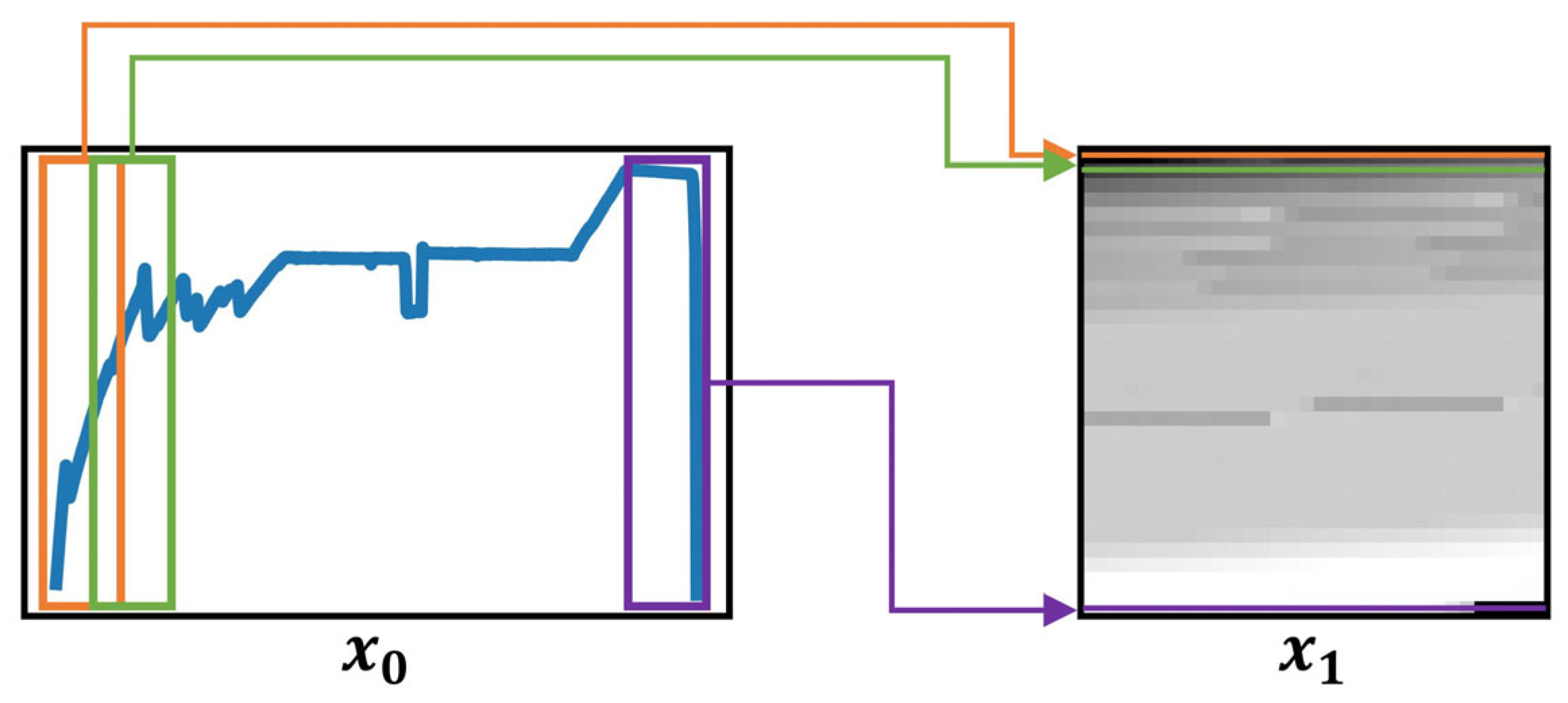
First, to better preserve temporal structure and local pattern continuity, each univariate time series is transformed into a two-dimensional grayscale image using an overlapping sliding window technique, as described in
Section 3.2. This transformation enables the use of convolutional operations that are sensitive to spatial and temporal locality, thus enhancing the network’s ability to extract meaningful sequence features.
Second, the fully connected layers in the original IDEC architecture are replaced with a deep convolutional autoencoder (DCAE). The encoder component is composed of convolutional and pooling layers, while the decoder consists of deconvolutional and upsampling layers. This architectural shift enables the network to leverage local translation-invariant features and scale more effectively with larger datasets, both of which are essential for analyzing long-duration operational sequences from industrial processes.
Third, TS-IDEC introduces a dual-mode clustering strategy. A soft clustering layer, based on Student’s t-distribution kernel, is used during training to refine latent representations while preserving cluster structure [
9]. In parallel, a hard clustering approach, based on the k-means algorithm, is applied to the same latent space after training to improve cluster separation. These two outputs, denoted as
(soft) and
(hard), are subsequently evaluated using a robust internal metric, and the better-performing result is selected as the final clustering solution (see
Section 3.5).
After defining the architectural components, it is important to clarify how the training and clustering output selection are performed. TS-IDEC is optimized by minimizing a joint loss function composed of a reconstruction loss, denoted
, and a clustering loss, denoted
. The reconstruction loss ensures that the autoencoder learns structure-preserving latent representations from the grayscale image input, while the clustering loss refines those representations to improve cluster compactness and separation. The combined loss function is optimized using stochastic gradient descent. Upon convergence, the model produces two candidate clustering results: a soft assignment output
derived from the probabilistic clustering layer, and a hard clustering output
generated by applying the k-means algorithm to the latent space. A two-stage evaluation procedure, based on qualitative consistency and a composite internal metric (see
Section 3.5), is used to select the better-performing result. The final output is denoted as
, representing the clustering result that balances accuracy and reliability.
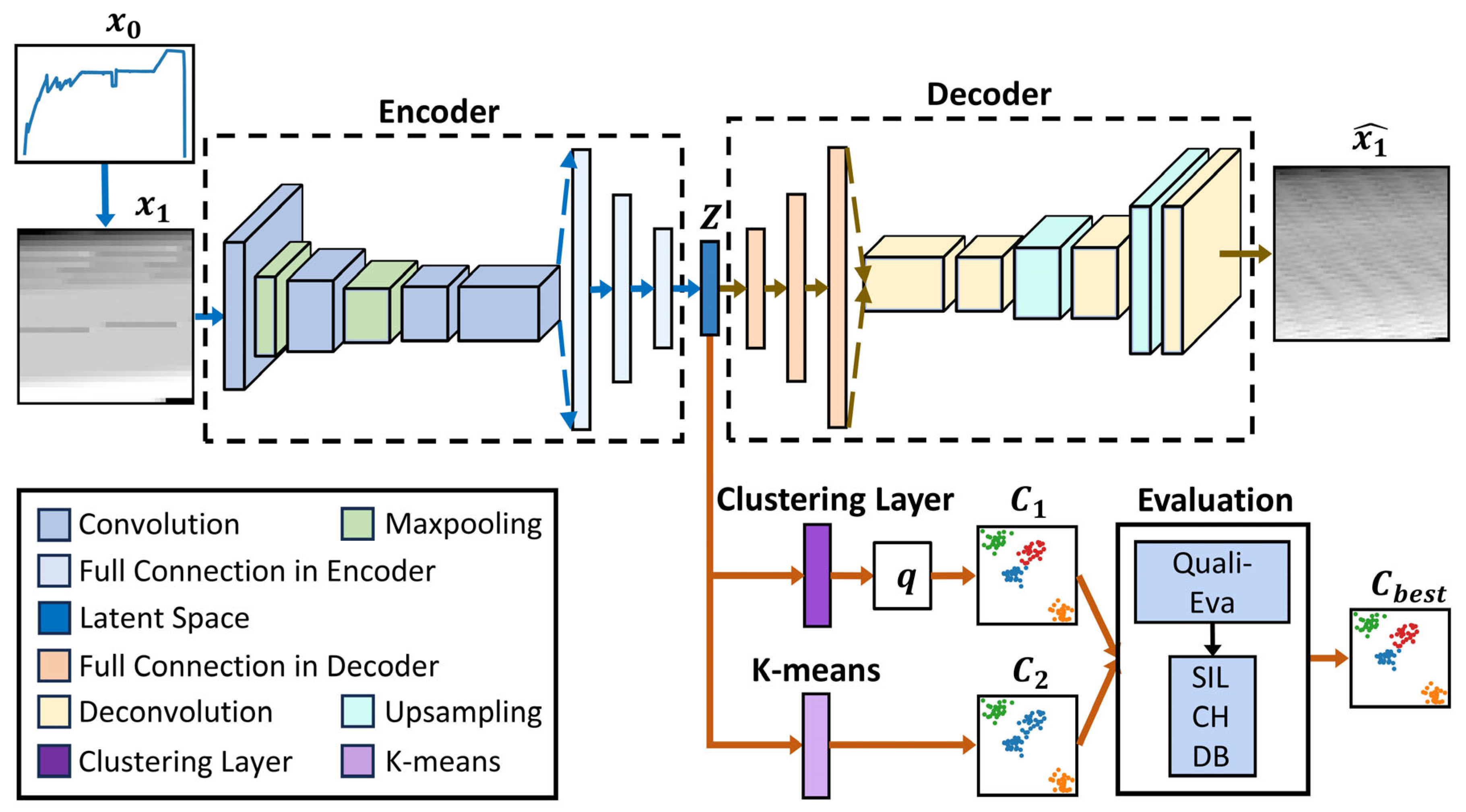
The complete architecture of TS-IDEC is illustrated in
Figure 1. The input time series
is first transformed into a grayscale matrix
, which serves as the input to the convolutional encoder. The encoder maps this input to a latent representation
, which is simultaneously used for reconstruction through the decoder and for clustering through both soft and hard assignment pathways. The training process jointly minimizes a reconstruction loss and a clustering loss, ensuring that latent representations are both compact and cluster-discriminative.
This architectural design makes TS-IDEC particularly suitable for industrial time-series clustering, where data are often unlabeled, irregular, and sensitive to small operational variations. The integration of time-series-aware input transformation, deep spatial-temporal feature learning, and dual clustering evaluation ensures the framework provides a robust and scalable solution for process pattern discovery.
3.3. Deep Convolutional Autoencoder and Clustering Mechanism
The core of the TS-IDEC framework is a deep convolutional autoencoder (DCAE), which is responsible for learning compact and informative latent representations of time-series input transformed into grayscale matrices. As shown in
Figure 1, the DCAE comprises three main components: an encoder, a latent space, and a decoder. This structure allows the model to learn spatial-temporal features that reflect both local and global process dynamics, which are essential for effective clustering.
Let the transformed 2D input be denoted . The encoder maps each input sample to a latent representation through a series of convolutional and pooling layers, defining a nonlinear transformation . This latent space preserves the most salient features of the time-series input while reducing its dimensionality. The decoder applies the inverse transformation using deconvolution and upsampling layers to reconstruct the original input. The reconstruction ensures that the latent features retain meaningful temporal structure and are not arbitrarily compressed.
The architectural parameters of the DCAE were selected through iterative testing to balance reconstruction fidelity with clustering effectiveness. The final configuration is summarized in
Table A1, which lists each layer’s type, kernel size, stride, padding, and activation function. The latent dimensionality was fixed at 128 based on experimental evaluation of compression quality and clustering performance.
Once the latent space
is learned, clustering is performed using a dual-mode strategy. The first mode is a soft clustering mechanism, implemented through a Student’s
t-distribution kernel as proposed by [
9]. Given the initial
cluster centroids
obtained through a simple clustering algorithm such
-means clustering and the data points
from the latent space
, the probability of assigning a sample
to cluster
, with centroid
, is computed as:
where
refers to the degree-of-freedom parameter of the t-distribution,
denotes the probability of assigning sample
to cluster
, and
denotes the Euclidean norm. This soft assignment matrix
is used to refine cluster assignments during training and contributes directly to the clustering loss (see
Section 3.4). Each sample is assigned to its most probable cluster according to
, forming the soft clustering output
.
The second mode is hard clustering, performed by applying the standard k-means algorithm directly to the latent space after training. This produces a second candidate output , which is typically more stable for deployment in industrial decision systems.
Next, to evaluate the clustering quality of
and
, a two-step evaluation approach is employed. The first stage involves qualitative assessment. In some experiments with complex datasets, the data points may not be well separated. For example, the soft clustering result
may consist of only one cluster, or a hard clustering result
may contain certain clusters with an extremely small number of data points. If one of these results is suboptimal based on the predefined clustering settings and requirements, the other is directly selected as the superior clustering result, denoted as
. If both exhibit similar performance in the qualitative assessment, a subsequent quantitative evaluation is performed. In this step, to determine the most appropriate final clustering output, both
and
are evaluated using a composite evaluation score integrating the Silhouette Score (SIL), Calinski–Harabasz Index (CH), and Davies–Bouldin Index (DB), as discussed in
Section 3.5. The better-performing output is selected as
. This two-stage evaluation ensures that the final clustering solution is both quantitatively sound and domain-explainable, which is essential for decision support in industrial applications.
This architecture can improve robustness to noise, enhance pattern separation, and explain operational modes for time-series data in complex industrial environments due to the joint leverage of the strength of convolutional representation learning and dual clustering comparison.
3.5. Composite Internal Evaluation Without Ground Truth
In the absence of labeled data, the evaluation of clustering performance relies on internal validation metrics that assess the compactness and separation of clusters based solely on the input data structure. While widely used, individual internal metrics often yield conflicting or unstable results, particularly when applied to high-dimensional, noisy, and irregular time-series data, which is typical in industrial contexts. To overcome this limitation, this paper proposes a composite internal evaluation strategy that integrates multiple standard metrics into a unified, normalized score, enabling robust and interpretable model selection.
This paper focuses on three widely used internal clustering indices: the Silhouette Score (SIL) [
13], the Calinski–Harabasz Index (CH) [
14], and the Davies–Bouldin Index (DB) [
15]. These metrics capture complementary aspects of clustering quality—cohesion, separation, and compactness—but differ in scale, sensitivity to outliers, and response to cluster shape and density. As shown in earlier studies [
37], no single metric performs consistently across all datasets, and metric-specific biases can distort evaluation outcomes in unsupervised settings.
To construct a robust evaluation score, this paper applies a two-stage normalization and aggregation procedure. First, each metric is rescaled using min–max normalization, with outlier effects mitigated through interquartile range (IQR) filtering. Then, each score is converted into a rank-based value, which reduces the influence of scale and irregular distributions. The final normalized score for each metric
is computed as the average of its min–max scaled and rank-normalized forms:
where
denotes the scores obtained after applying min-max scaling to the values with outliers removed, and
refers to the scores after applying rank normalization to the original evaluation scores, where
corresponding to the three evaluation metrics.
Let
denote the original vector of scores and
the same vector with outliers removed using IQR filtering. The min–max normalized score
is computed differently depending on whether higher or lower values indicate better clustering:
The rank-normalized score
is defined as:
where
is the rank of
in a sorted order and
refers to the number of values in the dataset. If
,
is computed in ascending order, whereas if
,
is computed in descending order.
Finally, the composite evaluation score
is calculated by averaging the normalized scores across all three metrics:
Based on the calculation in Equations (12)–(15), is in the range , and a higher value indicates a better clustering performance.
This composite score is used to select the final clustering result
from the two candidate outputs produced by TS-IDEC. Specifically, if the soft clustering result both
and the hard clustering result
yield distinct scores, the result with the higher
is selected. Additionally, this composite score is also employed to compare the performance of the TS-IDEC algorithm with the baseline methods and determine the optimal number of clusters in the absence of ground truth in
Section 5.
5. Experimental Evaluation and Analysis
This section presents a comprehensive evaluation of the proposed TS-IDEC framework through benchmark comparisons, domain-specific clustering analysis, robustness testing, and ablation studies. The experiments aim to (i) assess TS-IDEC’s performance relative to classical and deep clustering methods, (ii) examine the quality and explainability of furnace operational clusters, (iii) validate the framework’s stability under parameter variation, and (iv) justify the architectural and evaluation design choices through controlled ablations. All experiments are conducted on real-world univariate temperature time-series data collected from an industrial foundry, as described in
Section 4.
5.2. Benchmark Comparison: TS-IDEC vs. Baselines
To assess the clustering performance of TS-IDEC, this paper conducted a comparative evaluation against seven baseline algorithms introduced in
Section 5.1. All methods were tested on the standardized furnace melting dataset using the same experimental conditions. Performance was evaluated using the proposed composite internal metric
, which integrates the Silhouette Score (SIL), Calinski–Harabasz Index (CH), and Davies–Bouldin Index (DB), as described in
Section 3.5.
Each algorithm was allowed to search for the optimal number of clusters within the range representation
, and the best performing result based on
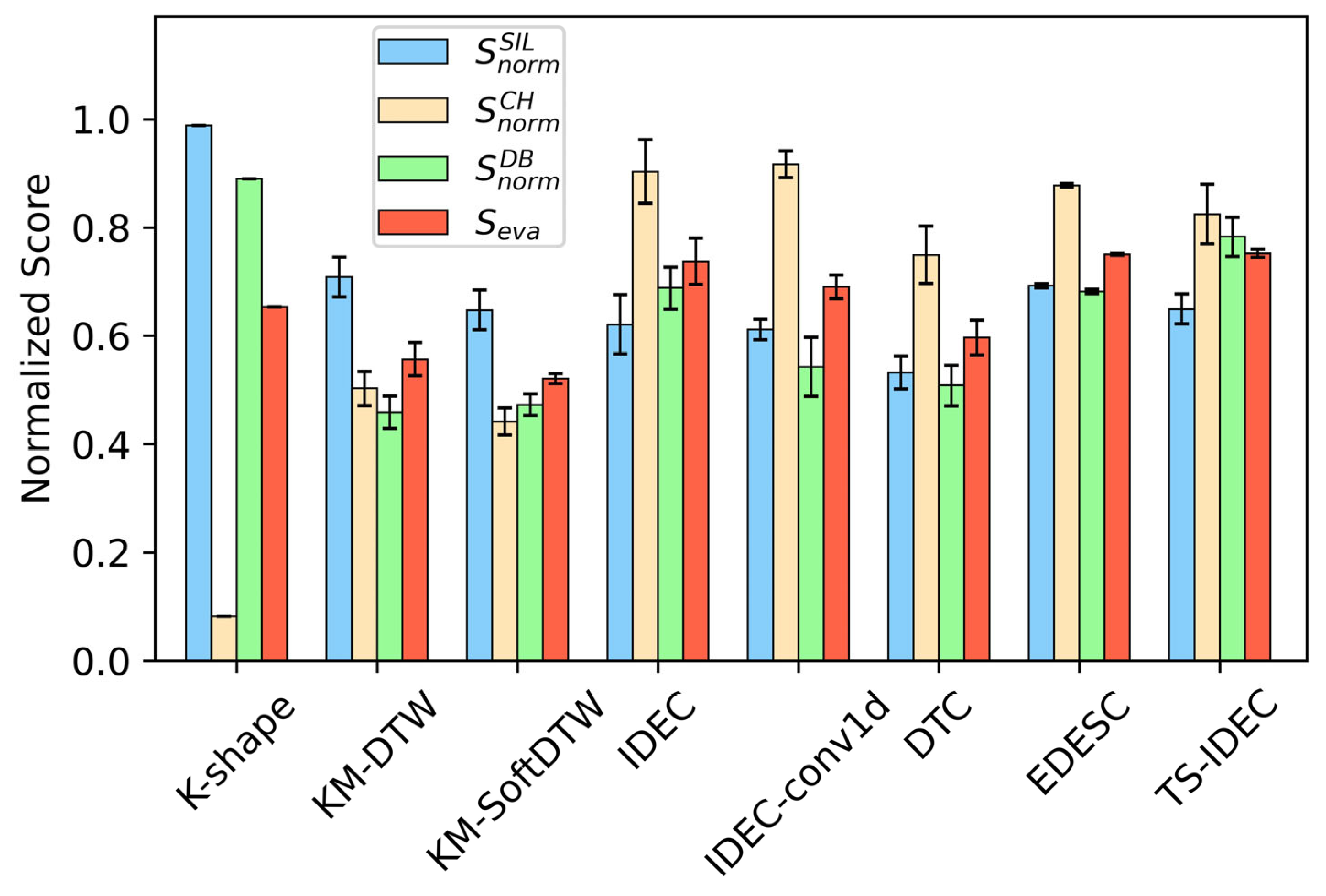
was reported. The evaluation scores are summarized in
Table 4 and visualized in
Figure 5.
The results in
Table 4 and
Figure 5 indicate that TS-IDEC achieves the highest overall performance based on the composite evaluation score
= 0.7523, outperforming all baselines, including state-of-the-art deep clustering methods such as IDEC and EDESC.
While TS-IDEC does not rank first in any of the individual normalized metrics, including , and , it consistently ranks second or third across all three, highlighting its robustness and stability across diverse evaluation dimensions. In contrast, methods such as k-Shape and IDEC attain superior results on specific indices but show limitations in practical interpretability. For instance, k-Shape frequently merges sequences with distinct melting modes into a single cluster, yielding higher , but obscuring meaningful process differences. Likewise, IDEC often produces compact clusters that score well on yet collapse the majority of sequences into a single group. In contrast, TS-IDEC achieves a balanced performance across all indices while preserving operational distinctions, making it both robust and practically interpretable.
Among deep baselines, IDEC and EDESC show competitive performance, with EDESC scoring slightly higher in than IDEC. However, both are outperformed by TS-IDEC, which integrates convolutional feature extraction, dual-mode clustering, and composite evaluation into a unified pipeline. The superior DB score of TS-IDEC suggests that its clusters are not only compact but also well-separated, even in the presence of overlapping operational modes and nonstationary behavior. Moreover, TS-IDEC outperforms both IDEC and IDEC-conv1D, demonstrating that the proposed image-based transformation provides more effective feature representation for clustering time-series data.
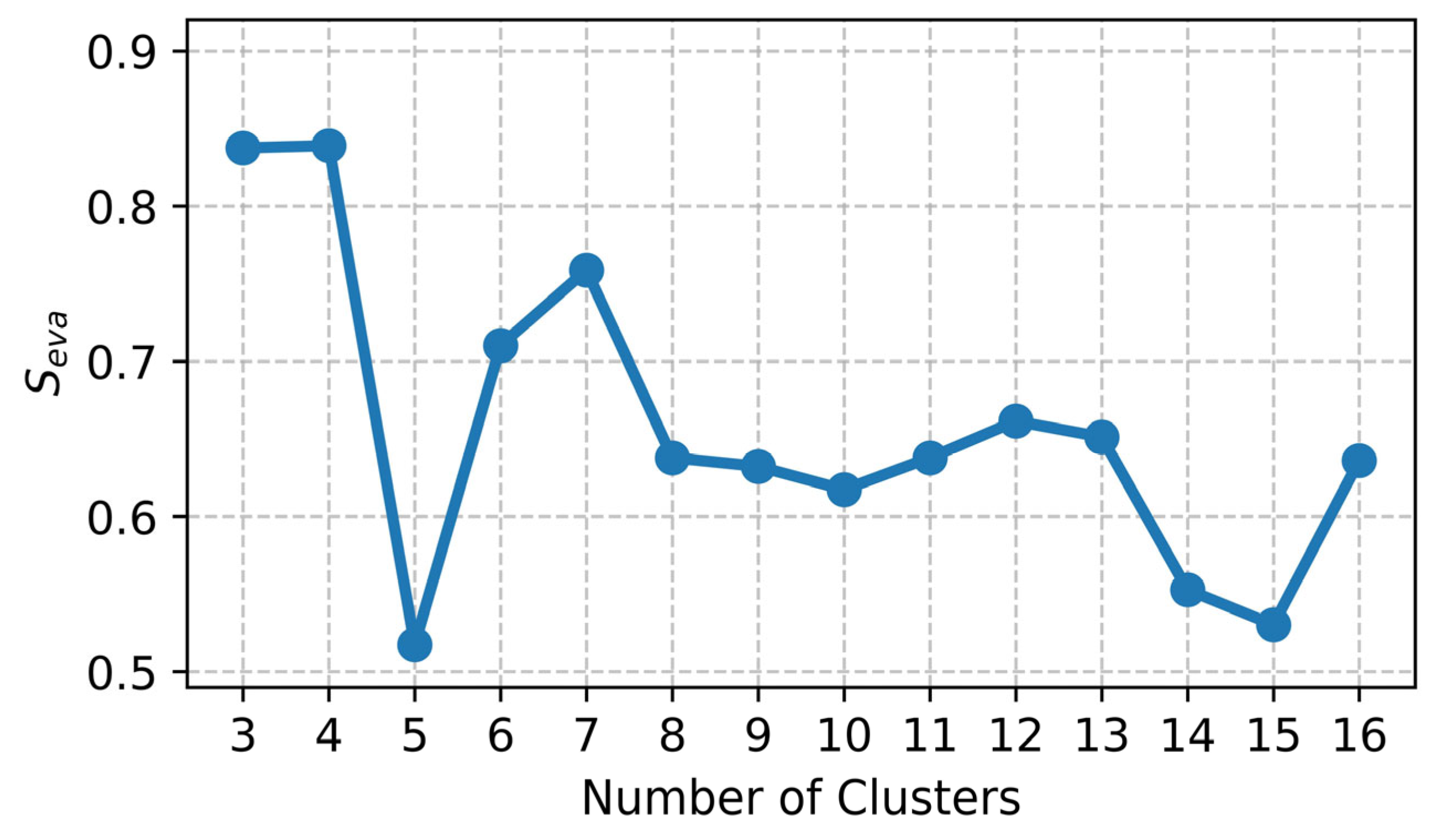
Importantly, the optimal cluster number selected for TS-IDEC is four, as determined by maximizing , while other methods tend to prefer fewer clusters. This indicates that TS-IDEC is capable of capturing finer operational distinctions that may be missed by more rigid or assumption-heavy algorithms.
Overall, these findings validate the effectiveness and generalizability of TS-IDEC in real-world, label-free industrial settings. Its balanced performance across cohesion, separation, and compactness metrics makes it particularly suitable for applications requiring effective unsupervised learning, such as energy efficiency profiling and process optimization in manufacturing.
5.3. Cluster Explanation in Furnace Operations
After validating the performance of TS-IDEC through benchmark comparisons, this study analyzes the operational clusters discovered in the foundry melting dataset. These clustering outcomes reveal distinct temperature dynamics and energy-use profiles across different melting operations, offering insights into real-world industrial behavior.
Figure 6 presents the composite evaluation scores
achieved by TS-IDEC across different numbers of clusters. While the optimal result was observed at four clusters, local maxima at seven and twelve clusters suggest the presence of meaningful substructure in the data.
To further explore cluster explainability, this research examines three configurations, including four, seven, and twelve clusters, using both low-dimensional visualization and statistical summaries.
The t-SNE plots in
Figure 7 show the latent representations of the time-series data projected into two dimensions for each cluster configuration. Each dot represents a single melting operation, and colors denote cluster membership.
The four-cluster solution (
Figure 7a) shows relatively well-separated groups, but some overlap regions remain, indicating soft transitions or outliers. The seven-cluster solution (
Figure 7b) provides finer granularity, with better intra-cluster compactness and inter-cluster separation. This configuration strikes a balance between model complexity and explainability. In contrast, the twelve-cluster result (
Figure 7c)—obtained from a failed 12-cluster run where one cluster collapsed—shows excessive fragmentation and increased overlap, reducing explainability.
Table 5 provides a quantitative comparison of distinct clustering configurations for objective judgment. The dominant cluster ratio measures the share of samples in the largest cluster. Standard deviation reflects imbalance across cluster sizes. The number of small clusters indicates over-fragmentation, defined here as clusters containing less than 1% of the data.
The results in
Table 5 highlight clear trade-offs across the three candidate solutions. At k = 4, more than half of all samples (53.6%) fall into a single dominant cluster, with the highest standard deviation (650.1), indicating strong imbalance and loss of granularity. At the other extreme, k = 12 produces four very small clusters (<1% of data each), suggesting over-fragmentation and reduced stability. The intermediate solution, k = 7, achieves the lowest dominant cluster ratio (39.8%) and the lowest standard deviation (414.3), reflecting a more balanced distribution of samples across clusters without introducing spurious minor groups. These results support k = 7 as the most robust clustering solution, offering a compromise between compactness and granularity.
Figure 8 shows the average temperature profiles (cluster centers) for each configuration. These curves represent the dominant melting behavior of each cluster.
In all cases, the general structure of the melting operation is retained: a rapid heating phase followed by a slower convergence to a plateau. However, the clustering in
Figure 8 reveals key variations in peak temperatures, ramp-up gradients, holding durations, and cooling profiles. These variations reflect underlying process differences such as material type, batch size, or operator behavior.
Table 6 summarizes key operational statistics for the seven-cluster configuration, which was selected for in-depth explainability based on the trade-off between granularity and clarity.
Cluster 0 is the most prevalent pattern, covering over one-third of the dataset. Cluster 6 is the least frequent but exhibits the longest average duration (7481.9 s), likely representing complex or delayed operations. Clusters 1 and 3 represent energy-use extremes: Cluster 1 shows the highest energy efficiency (325.0 kWh/tonne), while Cluster 3 consumes the most energy per unit (415.2 kWh/tonne), potentially indicating suboptimal or resource-intensive melting conditions.
These variations illustrate TS-IDEC’s ability to uncover operationally significant regimes that can inform energy optimization, operator training, or process standardization. The separation of long-duration, inefficient batches from short, efficient ones could support targeted investigations or recommendations.
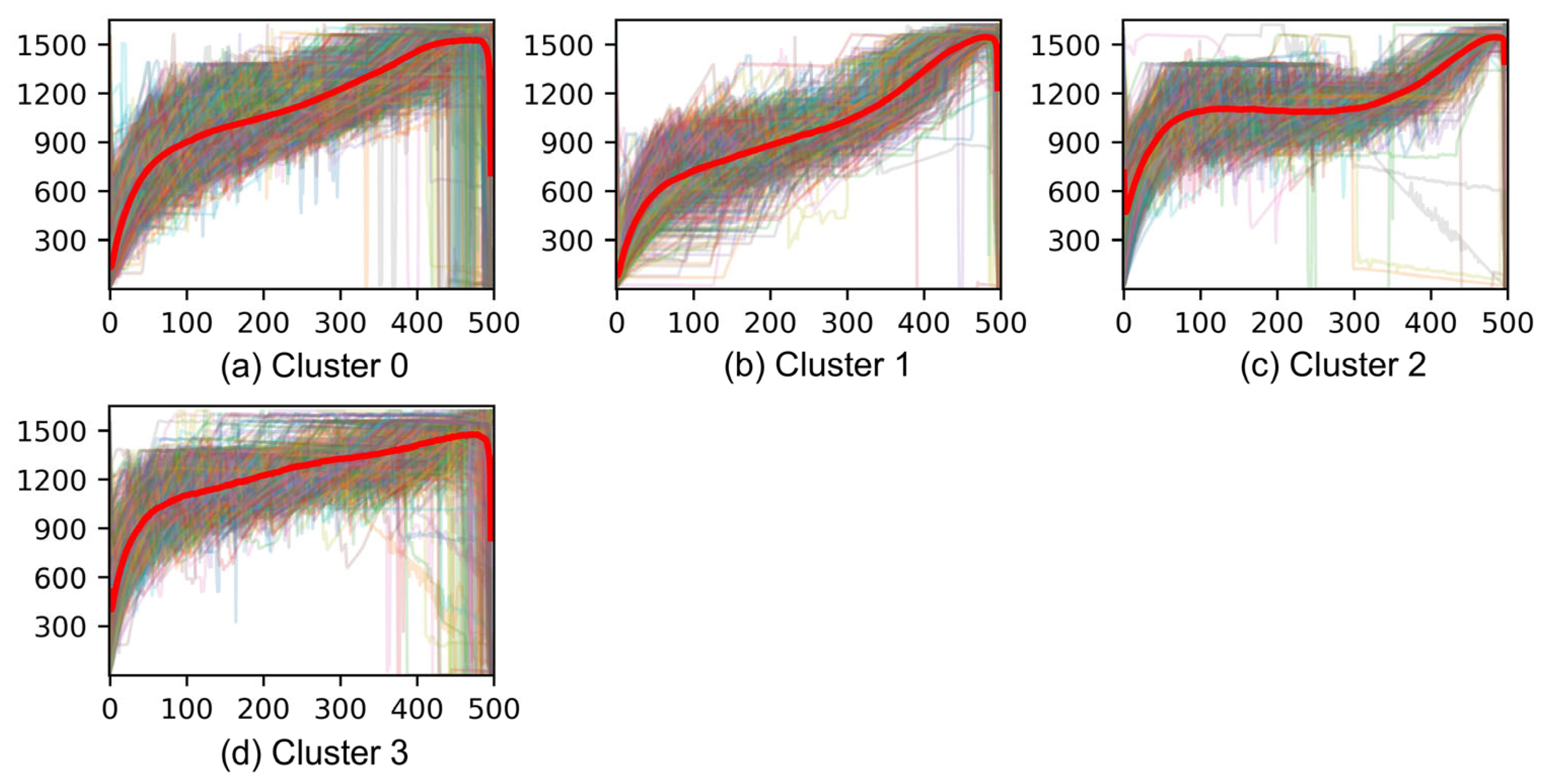
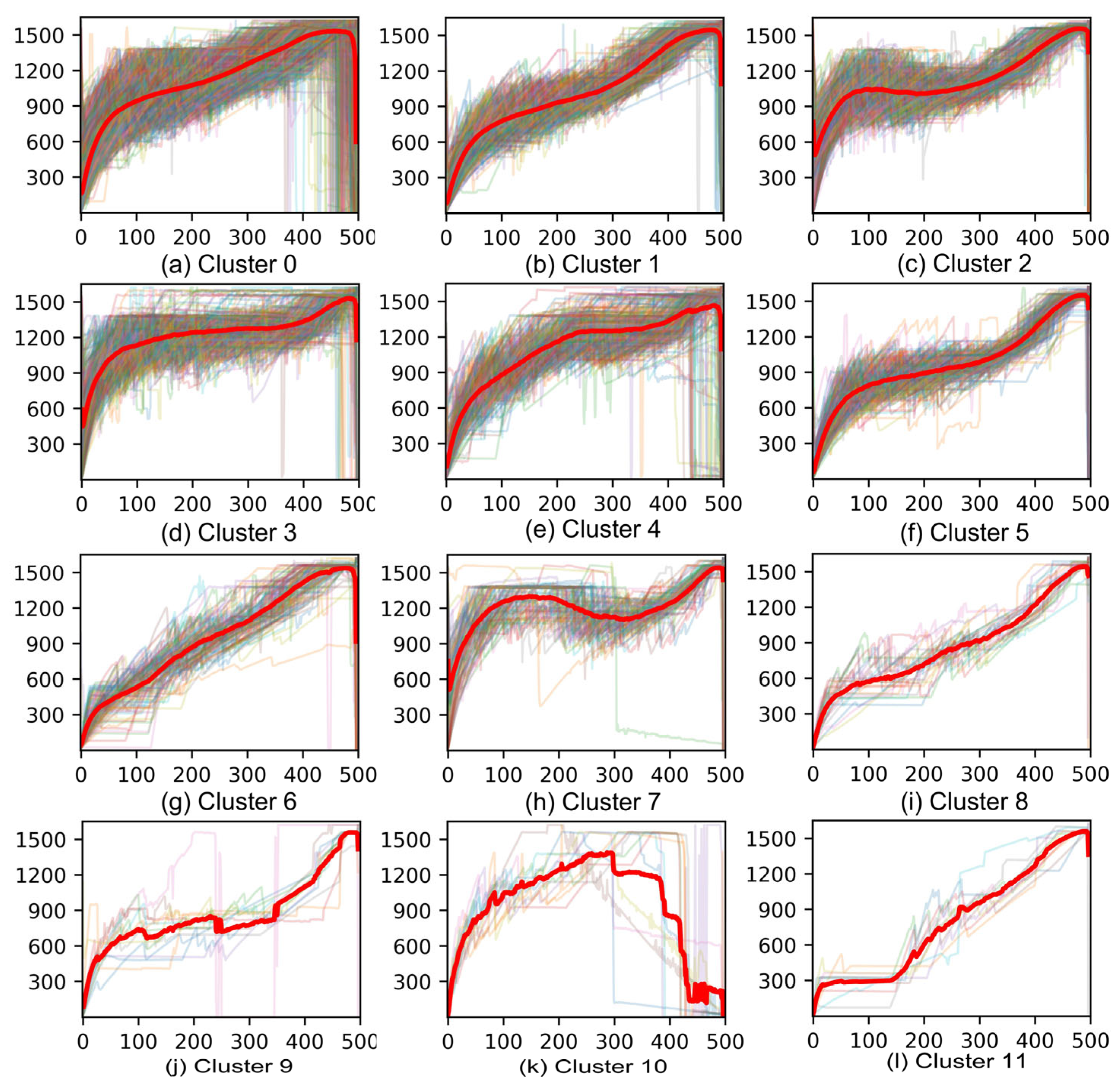
To further illustrate the temporal dynamics captured by the TS-IDEC model, detailed cluster-wise sequence plots are provided in
Figure A1,
Figure A2 and
Figure A3 in the
Appendix A. Each figure overlays all melting operation time series within a cluster configuration (4, 7, and 12 clusters), with the cluster centers highlighted in red. These visualizations reveal the degree of intra-cluster coherence and the diversity of temporal profiles across clusters. In particular, they confirm that TS-IDEC is capable of grouping sequences with similar thermal behaviors, while also maintaining separation between distinctly patterned operations. The increased fragmentation observed in the 12-cluster case (
Figure A3) further supports the explainability argument made in favor of the 7-cluster configuration.
7. Conclusions
This paper presents TS-IDEC, a novel deep time-series clustering framework for uncovering hidden operational patterns in complex, unlabeled industrial datasets. By transforming univariate time series into grayscale matrices through overlapping sliding windows, the framework enables convolutional neural networks to extract spatial–temporal features. TS-IDEC integrates a deep convolutional autoencoder with a dual-mode clustering strategy, combining soft and hard assignments, and selects the final result Via a two-stage mechanism guided by a composite evaluation score.
To address limitations in existing unsupervised clustering evaluation methods, this paper proposes a data-driven composite metric, , which integrates normalized SIL, CH and DB indices. This metric reduces inconsistencies between individual scores and ensures stable model selection in the absence of ground truth. Comparative experiments demonstrated that TS-IDEC consistently outperforms classical methods (e.g., k-means-DTW, k-shape), deep clustering baselines (e.g., IDEC, DTC, EDESC), and convolutional variants (e.g., IDEC-conv1D).
Application to real-world furnace operations in a Nordic foundry confirmed the framework’s ability to identify meaningful and explainable melting modes. Seven distinct clusters are discovered, revealing systematic differences in energy efficiency, process duration, and thermal dynamics. These insights enable benchmarking of operational performance, detection of inefficiencies, and formulation of data-driven strategies for process optimization, energy savings, and workforce training.
Scientifically, TS-IDEC advances unsupervised time-series clustering by addressing three major challenges: handling variable-length sequences, reducing instability in soft clustering, and providing a consistent evaluation criterion. The framework combines image-based representation learning, dual-mode clustering resilience, and reproducible evaluation, thereby improving rigor and reliability in unstructured industrial settings.
Practically, TS-IDEC generates domain-aligned, explainable insights without labeled data or manual feature engineering, supporting its deployment in smart manufacturing environments. It enables large-scale benchmarking across thousands of unlabeled cycles and highlights energy-optimal operating modes and intervention-heavy batches.
Despite its strengths, the approach remains sensitive to the selection of cluster numbers, underscoring the difficulty of modeling overlapping or ambiguous regimes. Future research could integrate recent deep learning–based time-series clustering approaches, including Transformer and attention-based architectures, both to establish a more comprehensive benchmark against state-of-the-art methods and to potentially advance clustering performance. Further automation of the windowing transformation, extension to multivariate and multimodal time series, and integration with self-supervised learning may enhance robustness and generalizability. Furthermore, future work should validate the proposed composite metric against datasets with ground truth to further establish its robustness and generalizability. Finally, coupling TS-IDEC with explainable AI methods could deepen interpretability by linking discovered clusters to underlying process parameters and enabling human-in-the-loop decision support.
Author Contributions
Conceptualization, Z.M., B.N.J. and Z.G.M.; methodology, Z.M., B.N.J. and Z.G.M.; software, Z.M.; validation, Z.M.; formal analysis, Z.M.; investigation, Z.M.; resources, B.N.J. and Z.G.M.; data curation, Z.M.; writing—original draft preparation, Z.M.; writing—review and editing, Z.M., B.N.J. and Z.G.M.; visualization, Z.M.; supervision, B.N.J. and Z.G.M.; project administration, B.N.J. and Z.G.M.; funding acquisition, Z.G.M. All authors have read and agreed to the published version of the manuscript.
Funding
This work was funded by the Energy Technology Development and Demonstration Programme (EUDP) in Denmark under the “Data-driven best-practice for energy-efficient operation of industrial processes—A system integration approach to reduce the CO2 emissions of industrial processes” funded by EUDP (Case no.64022-1051).
Data Availability Statement
The data that supports the findings of this study were obtained from an industrial partner and are subject to confidentiality agreements. As such, the original dataset cannot be shared publicly. Researchers interested in the methodology or derived results may contact the corresponding author for further discussion or guidance on reproducing the framework using their own data.
Acknowledgments
During the preparation of this work, the authors used ChatGPT 4o to improve the readability and language of the manuscript. After using this tool, the authors reviewed and edited the content as needed and take full responsibility for the content of the published article.
Conflicts of Interest
The authors declare no conflicts of interest.
Abbreviations
The following abbreviations are used in this manuscript:
| CAE | Convolutional Autoencoder |
| CH | Calinski–Harabasz Index |
| DB | Davies–Bouldin Index |
| DCAE | Deep Convolutional Autoencoder |
| DEC | Deep Embedded Clustering |
| DEETO | Deep Embedding with Topology Optimization |
| DTC | Deep Temporal Clustering |
| DTW | Dynamic Time Warping |
| EDESC | Efficient Deep Subspace Clustering |
| GAN | Generative Adversarial Network |
| IDEC | Improved Deep Embedded Clustering |
| IQR | Interquartile Range |
| KL | Kullback–Leibler |
| MSE | Mean Squared Error |
| SIL | Silhouette Score |
| TS-IDEC | Time-Series Image-based Deep Embedded Clustering |
| soft-DTW | Soft Dynamic Time Warping |
References
- Howard, D.A.; Værbak, M.; Ma, Z.; Jørgensen, B.N.; Ma, Z. Data-driven digital twin for foundry production process: Facilitating best practice operations investigation and impact analysis. In Proceedings of the Energy Informatics Academy Conference, EI.A 2024, Bali, Indonesia, 23–25 October 2024; pp. 259–273. [Google Scholar]
- International Energy Agency. World Energy Outlook. 2024. Available online: https://www.iea.org/reports/world-energy-outlook-2024 (accessed on 15 March 2025).
- Howard, D.A.; Jørgensen, B.N.; Ma, Z. Identifying best practice melting patterns in induction furnaces: A data-driven approach using time series k-means clustering and multi-criteria decision making. In Proceedings of the Energy Informatics Academy Conference, EI.A 2023, Campinas, Brazil, 6–8 December 2023; pp. 271–288. [Google Scholar]
- Oyewole, G.J.; Thopil, G.A. Data clustering: Application and trends. Artif. Intell. Rev. 2023, 56, 6439–6475. [Google Scholar] [CrossRef] [PubMed]
- Ezugwu, A.E.; Ikotun, A.M.; Oyelade, O.O.; Abualigah, L.; Agushaka, J.O.; Eke, C.I.; Akinyelu, A.A. A comprehensive survey of clustering algorithms: State-of-the-art machine learning applications, taxonomy, challenges, and future research prospects. Eng. Appl. Artif. Intell. 2022, 110, 104743. [Google Scholar] [CrossRef]
- Jeong, Y.-S.; Jeong, M.K.; Omitaomu, O.A. Weighted dynamic time warping for time series classification. Pattern Recognit. 2011, 44, 2231–2240. [Google Scholar] [CrossRef]
- Paparrizos, J.; Gravano, L. k-shape: Efficient and accurate clustering of time series. In Proceedings of the 2015 ACM SIGMOD International Conference on Management of Data, Melbourne, Australia, 31 May 2015–4 June 2015; pp. 1855–1870. [Google Scholar]
- Li, D.; Liu, Y.; Huang, D.; Xu, C. A Semisupervised Soft-Sensor of Just-in-Time Learning With Structure Entropy Clustering and Applications for Industrial Processes Monitoring. IEEE Trans. Artif. Intell. 2022, 4, 722–733. [Google Scholar] [CrossRef]
- Xie, J.; Girshick, R.; Farhadi, A. Unsupervised deep embedding for clustering analysis. In Proceedings of the International Conference on Machine Learning, New York, NY, USA, 19–24 June 2016; pp. 478–487. [Google Scholar]
- Guo, X.; Gao, L.; Liu, X.; Yin, J. Improved deep embedded clustering with local structure preservation. In Proceedings of the Twenty-Sixth International Joint Conference on Artificial Intelligence, Melbourne, Australia, 19–25 August 2017; pp. 1753–1759. [Google Scholar]
- Madiraju, N.S.; Sadat, S.M.; Fisher, D.; Karimabadi, H. Deep temporal clustering: Fully unsupervised learning of time-domain features. arXiv 2018, arXiv:1802.01059. [Google Scholar] [CrossRef]
- Cai, J.Y.; Fan, J.C.; Guo, W.Z.; Wang, S.P.; Zhang, Y.H.; Zhang, Z. Efficient Deep Embedded Subspace Clustering. In Proceedings of the 2022 IEEE/CVF Conference on Computer Vision and Pattern Recognition (CVPR 2022), New Orleans, LA, USA, 18–24 June 2022; pp. 21–30. [Google Scholar] [CrossRef]
- Rousseeuw, P.J. Silhouettes: A graphical aid to the interpretation and validation of cluster analysis. J. Comput. Appl. Math. 1987, 20, 53–65. [Google Scholar] [CrossRef]
- Caliński, T.; Harabasz, J. A dendrite method for cluster analysis. Commun. Stat-Theory Methods 1974, 3, 1–27. [Google Scholar] [CrossRef]
- Davies, D.L.; Bouldin, D.W. A cluster separation measure. IEEE Trans. Pattern Anal. Mach. Intell. 1979, PAMI-1, 224–227. [Google Scholar] [CrossRef]
- International Energy Agency. Global Energy and Climate Model. Available online: https://www.iea.org/reports/global-energy-and-climate-model (accessed on 15 March 2025).
- European Foundry Federation. The European Foundry Industry. 2023. Available online: https://eff-eu.org/wp-content/uploads/2024/12/CAEF-Co7_2023-complete.pdf (accessed on 19 March 2025).
- Keramidas, K.; Mima, S.; Bidaud, A. Opportunities and roadblocks in the decarbonisation of the global steel sector: A demand and production modelling approach. Energy Clim. Change 2024, 5, 100121. [Google Scholar] [CrossRef]
- Jones, M.D.; Hutcheson, S.; Camba, J.D. Past, present, and future barriers to digital transformation in manufacturing: A review. J. Manuf. Syst. 2021, 60, 936–948. [Google Scholar] [CrossRef]
- Battistoni, E.; Gitto, S.; Murgia, G.; Campisi, D. Adoption paths of digital transformation in manufacturing SME. Int. J. Prod. Econ. 2023, 255, 108675. [Google Scholar] [CrossRef]
- Guijo-Rubio, D.; Duran-Rosal, A.M.; Gutierrez, P.A.; Troncoso, A.; Hervas-Martinez, C. Time-series clustering based on the characterization of segment typologies. IEEE T. Cybern. 2021, 51, 5409–5422. [Google Scholar] [CrossRef]
- Barrera, J.M.; Reina, A.; Mate, A.; Trujillo, J.C. Fault detection and diagnosis for industrial processes based on clustering and autoencoders: A case of gas turbines. Int. J. Mach. Learn. Cybern. 2022, 13, 3113–3129. [Google Scholar] [CrossRef]
- Berndt, D.J.; Clifford, J. Using dynamic time warping to find patterns in time series. In Proceedings of the 3rd International Conference on Knowledge Discovery and Data Mining, Seattle, WA, USA, 31 July 1994–1 August 1994; pp. 359–370. [Google Scholar]
- Cuturi, M.; Blondel, M. Soft-dtw: A differentiable loss function for time-series. In Proceedings of the International Conference on Machine Learning, Sydney, NSW, Australia, 6–11 August 2017; pp. 894–903. [Google Scholar]
- Suh, W.H.; Oh, S.; Ahn, C.W. Metaheuristic-based time series clustering for anomaly detection in manufacturing industry. Appl. Intell. 2023, 53, 21723–21742. [Google Scholar] [CrossRef]
- Nizam, H.; Zafar, S.; Lv, Z.; Wang, F.; Hu, X. Real-time deep anomaly detection framework for multivariate time-series data in industrial IoT. IEEE Sens. J. 2022, 22, 22836–22849. [Google Scholar] [CrossRef]
- Alqahtani, A.; Xie, X.; Deng, J.; Jones, M.W. A deep convolutional auto-encoder with embedded clustering. In Proceedings of the 2018 25th IEEE International Conference on Image Processing (ICIP), Athens, Greece, 7–10 October 2018; pp. 4058–4062. [Google Scholar]
- Lee, S.; Choi, C.; Son, Y. Deep time-series clustering via latent representation alignment. Knowl.-Based Syst. 2024, 303, 112434. [Google Scholar] [CrossRef]
- Mukherjee, S.; Asnani, H.; Lin, E.; Kannan, S. Clustergan: Latent space clustering in generative adversarial networks. In Proceedings of the AAAI Conference on Artificial Intelligence, Honolulu, HI, USA, 27 January–1 February 2019; pp. 4610–4617. [Google Scholar]
- Chen, X.; Duan, Y.; Houthooft, R.; Schulman, J.; Sutskever, I.; Abbeel, P. Infogan: Interpretable representation learning by information maximizing generative adversarial nets. Adv. Neural Inf. Process. Syst. 2016, 29, 2180–2188. [Google Scholar]
- Ji, P.; Zhang, T.; Li, H.; Salzmann, M.; Reid, I. Deep subspace clustering networks. Adv. Neural Inf. Process. Syst. 2017, 30, 23–32. [Google Scholar]
- Chen, R.; Yan, X.; Wang, S.; Xiao, G. DA-Net: Dual-attention network for multivariate time series classification. Inf. Sci. 2022, 610, 472–487. [Google Scholar] [CrossRef]
- Papavasileiou, P.; Giovanis, D.G.; Pozzetti, G.; Kathrein, M.; Czettl, C.; Kevrekidis, I.G.; Boudouvis, A.G.; Bordas, S.P.A.; Koronaki, E.D. Integrating supervised and unsupervised learning approaches to unveil critical process inputs. Comput. Chem. Eng. 2025, 192, 108857. [Google Scholar] [CrossRef]
- Castela Forte, J.; Yeshmagambetova, G.; van der Grinten, M.L.; Hiemstra, B.; Kaufmann, T.; Eck, R.J.; Keus, F.; Epema, A.H.; Wiering, M.A.; van der Horst, I.C. Identifying and characterizing high-risk clusters in a heterogeneous ICU population with deep embedded clustering. Sci. Rep. 2021, 11, 12109. [Google Scholar] [CrossRef] [PubMed]
- Eskandarnia, E.; Al-Ammal, H.M.; Ksantini, R. An embedded deep-clustering-based load profiling framework. Sust. Cities Soc. 2022, 78, 103618. [Google Scholar] [CrossRef]
- Lai, C.S.; Zhong, C.; Pan, K.; Ng, W.W.; Lai, L.L. A deep learning based hybrid method for hourly solar radiation forecasting. Expert Syst. Appl. 2021, 177, 114941. [Google Scholar] [CrossRef]
- Arbelaitz, O.; Gurrutxaga, I.; Muguerza, J.; Pérez, J.M.; Perona, I. An extensive comparative study of cluster validity indices. Pattern Recognit. 2013, 46, 243–256. [Google Scholar] [CrossRef]
- Ren, Y.Z.; Pu, J.Y.; Yang, Z.M.; Xu, J.; Li, G.F.; Pu, X.R.; Yu, P.S.; He, L.F. Deep clustering: A comprehensive survey. IEEE Trans. Neural Netw. Learn. Syst. 2024, 36, 5858–5878. [Google Scholar] [CrossRef] [PubMed]
- Kingma, D.P.; Ba, J. Adam: A method for stochastic optimization. arXiv 2014, arXiv:1412.6980. [Google Scholar]
- Ma, Z.; Jorgensen, B.N.; Ma, Z.G. A systematic data characteristic understanding framework towards physical-sensor big data challenges. J. Big Data 2024, 11, 84. [Google Scholar] [CrossRef]
- Tavenard, R.; Faouzi, J.; Vandewiele, G.; Divo, F.; Androz, G.; Holtz, C.; Payne, M.; Yurchak, R.; Rußwurm, M.; Kolar, K. Tslearn, a machine learning toolkit for time series data. J. Mach. Learn. Res. 2020, 21, 1–6. [Google Scholar]
- Paszke, A.; Gross, S.; Massa, F.; Lerer, A.; Bradbury, J.; Chanan, G.; Killeen, T.; Lin, Z.; Gimelshein, N.; Antiga, L. Pytorch: An imperative style, high-performance deep learning library. Adv. Neural Inf. Process. Syst. 2019, 32, 8026–8037. [Google Scholar]
- Alqahtani, A.; Ali, M.; Xie, X.H.; Jones, M.W. Deep time-series clustering: A review. Electronics 2021, 10, 3001. [Google Scholar] [CrossRef]
- Schubert, E. Stop using the elbow criterion for k-means and how to choose the number of clusters instead. SIGKDD Explor. 2023, 25, 36–42. [Google Scholar] [CrossRef]
Figure 1.
Architecture of the TS-IDEC network. The pipeline includes overlapping sliding window transformation, convolutional encoder, latent space extraction, decoder, and dual clustering modules. Color-coded blocks denote functional components.
Figure 2.
Example of overlapping sliding window transformation. The original univariate time series is segmented into overlapping windows (left), which are stacked into a grayscale matrix (right) suitable for convolutional feature extraction.
Figure 3.
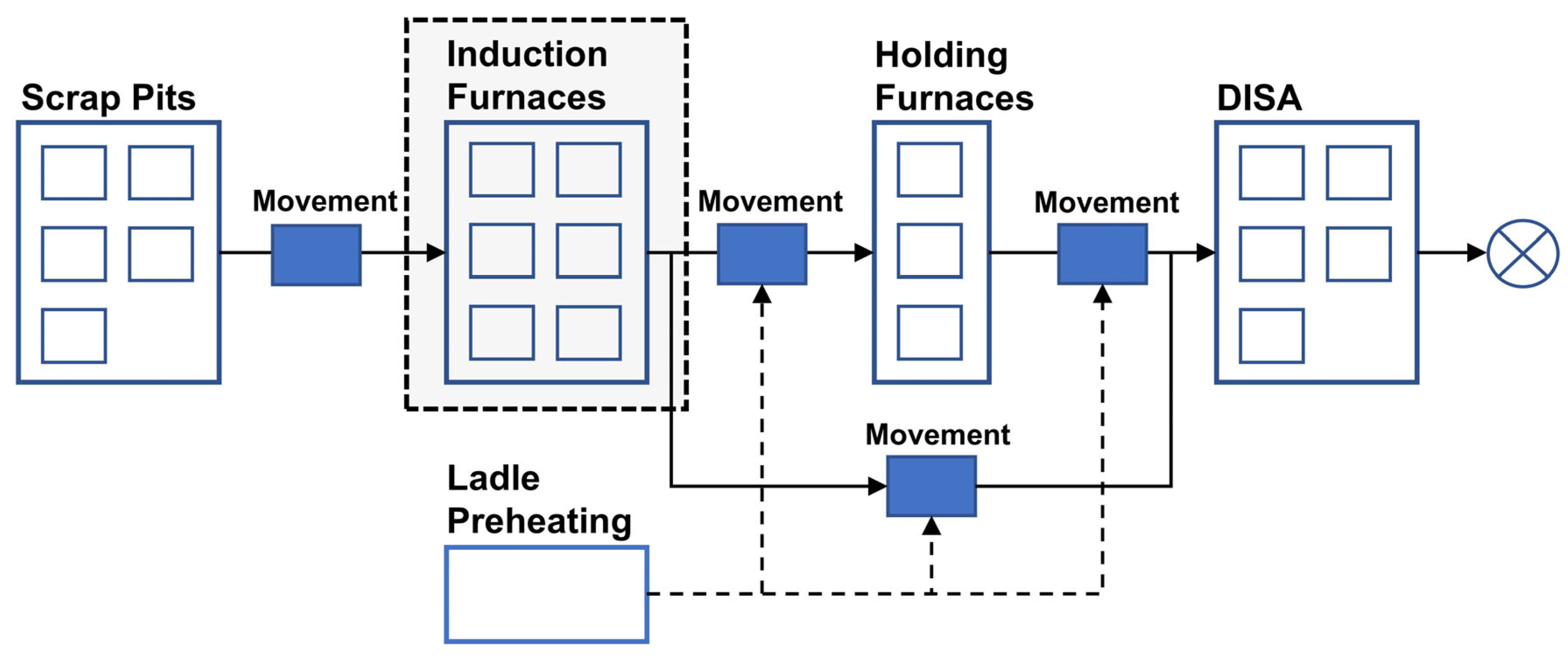
Industrial processing operations in the foundry.
Figure 4.
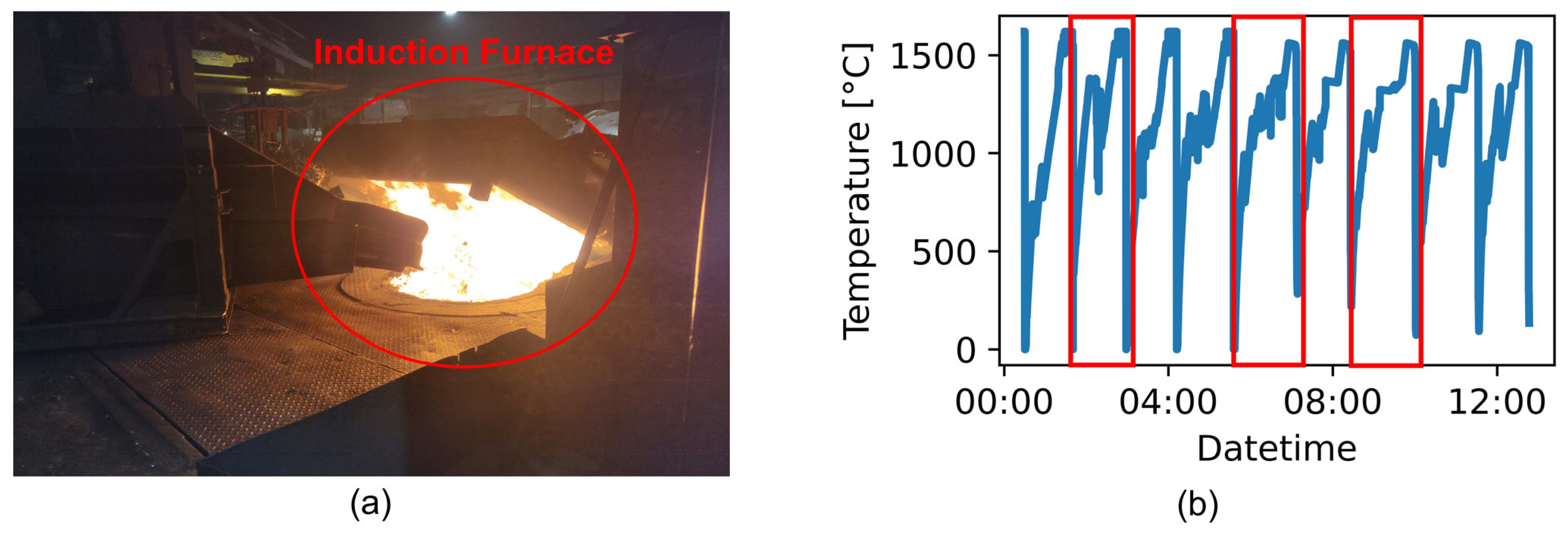
(a) Selected induction furnace used in the case study. (b) Sample temperature profile of a complete melting operation, where the blue curve represents the melting operation over time, and the red boxes highlight individual melting cycles.
Figure 5.
Normalized evaluation scores of different algorithms. The x-axis represents the names of algorithms, where “KM” denotes k-means. The y-axis shows the normalized scores ranging from 0 to 1. Each group of four bars corresponds to distinct evaluation metrics, as indicated in the legend, with error bars representing the standard error of repetitions.
Figure 6.
Normalized evaluation scores of different numbers of clusters for the TS-IDEC algorithm.
Figure 7.
The t-SNE illustration of TS-IDEC clustering results in different numbers of clusters. Subfigures (a–c) depict the clustering outcomes for 4, 7 and 12 clusters, respectively. Each solid data point represents a time series projected into the t-SNE space, with colors indicating cluster assignments as defined in the legend.
Figure 8.
The cluster centers of TS-IDEC clustering with different numbers of clusters. Subfigures (a–c) depict the clustering outcomes for 4, 7 and 12 clusters, respectively. In each subfigure, the x-axis refers to the sequential data points, and the y-axis denotes furnace temperature (°C). Each curve represents a cluster center, with colors indicating cluster assignments as defined in the legend.
Figure 9.
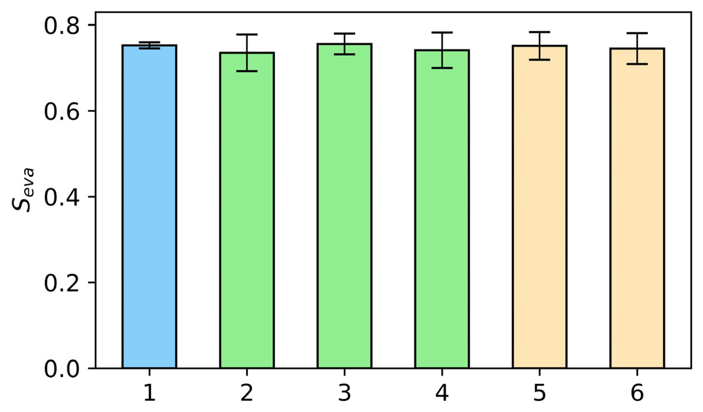
Evaluation scores of different experiments for sensitivity analysis. The x-axis corresponds to the experiment indices as presented in
Table 6, while the y-axis indicates the evaluation score
. The light blue bars represent the default configuration, the light green bars illustrate experiments analyzing the impact of stride, and the light orange bars depict experiments assessing the effect of varying the window size. The error bars represent the standard error of repetitions.
Figure 10.
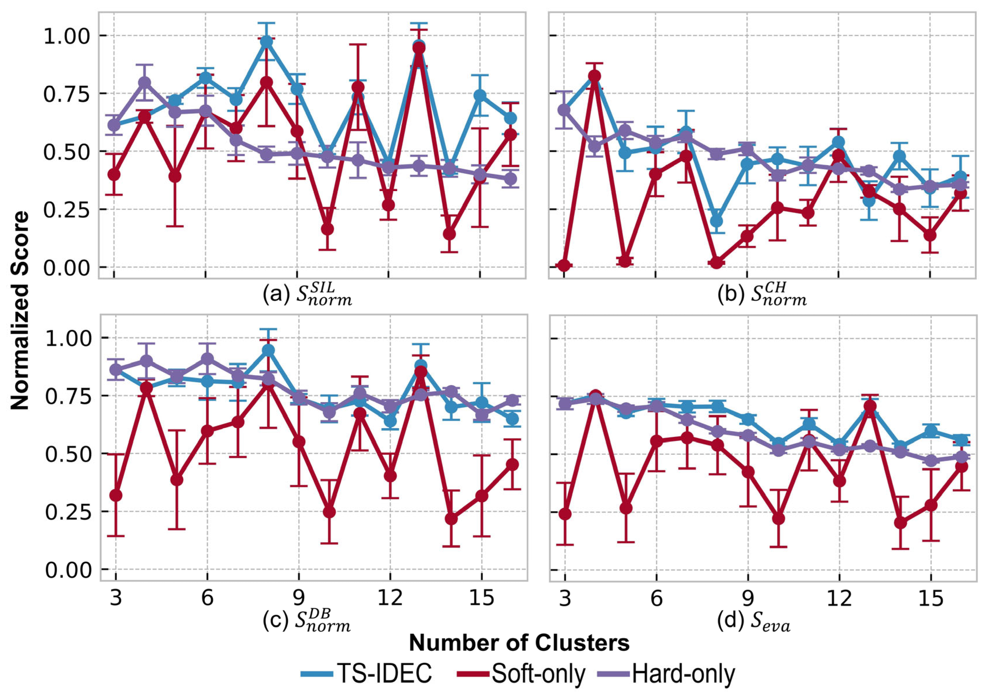
Evaluation scores of clustering ablation study. X-axes denote the number of clusters, and y-axes refer to the normalized evaluation scores. Sub-figures (a–d) represents the four evaluation scores , , and , respectively. Three lines stand for the methods shown in the legend, respectively, and error bars are the standard deviation of repetitions.
Table 1.
Comparison of Deep Clustering Approaches for Industrial Time-Series Data.
| Clustering Approach | Representative Methods | Strengths | Limitations | Suitability for Industrial Time-Series |
|---|
| Autoencoder-based | DEC [9]; IDEC [10] | Joint feature learning and clustering; low-dimensional embeddings | Often assumes independently and identically distributed data; ignores temporal dependencies | Moderate: needs adaptation for sequence learning |
| Convolutional Autoencoder | DCAE [27]; TS-IDEC (this study) | Learns localized spatial/temporal patterns; scalable to image-structured input | Performance depends on image transformation quality | High: effective after converting the time-series to image representations |
| GAN-based | ClusterGAN [29]; InfoGAN [30] | Captures complex distributions; good for generative synthesis | Training instability | Low: rarely used for time-series due to mode collapse and training cost |
| Subspace clustering | EDESC [12]; Deep Subspace Clustering [31] | Models latent subspaces; scalable; suitable for high-dimensional data | Less effective when a strong temporal order exists | Moderate: best for multivariate sensor data, not univariate signals |
| Topology-aware | DEETO [28]; DA-Net [32] | Preserves geometric and topological structure in the latent space | High complexity; difficult to scale; sensitive to hyperparameters | Low to Moderate: promising for structured data but immature for industry |
Table 2.
Comparison of Internal Clustering Evaluation Metrics.
| Metric | Core Idea | Output Range | Strengths | Limitations | Suitability for Time-Series Clustering |
|---|
| Silhouette Score (SIL) | Balance between cohesion and separation | [−1, 1] | Intuitive; interpretable; shape-agnostic | Suffers in high dimensions; may penalize non-convex clusters | Moderate: interpretable but sensitive to time warping |
| Calinski–Harabasz (CH) | Ratio of between- to within-cluster variance | [0, ∞) | Computationally efficient; works well for spherical clusters | Biased toward higher cluster counts; assumes isotropic structure | Moderate: fast but sensitive to density imbalance |
| Davies–Bouldin (DB) | Average similarity between each cluster and its nearest | [0, ∞) | Low values favor compact, well-separated clusters | Sensitive to outliers and centroid instability | Moderate: useful but unreliable with noise |
| Dunn Index | Ratio of minimum inter-cluster to maximum intra-cluster | [0, ∞) | Encourages compactness and separation | Highly sensitive to noise and outliers; rarely stable | Low: rarely used in noisy industrial settings |
| Entropy-based indices | Based on cluster label uncertainty | N/A | Captures uncertainty and distributional overlap | Requires discretization; less interpretable | Low: useful in hybrid methods or fuzzy clustering |
| Composite Scores | Weighted/normalized combination of metrics | [0, 1] (typical) | Mitigates individual biases; balances trade-offs | Requires normalization and weighting schemes; no standard method | High: best suited for unsupervised industrial analytics |
Table 3.
Overview of Time Series Clustering Algorithms Used for Benchmarking.
| Algorithm | Reference | Description |
|---|
| k-Shape | [7] | A shape-based clustering algorithm using normalized cross-correlation. |
| k-Means-DTW | [6] | Classical k-means applied with Dynamic Time Warping (DTW) distance. |
| k-Means-SoftDTW | [24] | A differentiable version of DTW that allows smooth optimization. |
| IDEC | [10] | A deep-embedded clustering method using fully connected autoencoders and soft assignment. |
| IDEC-conv1D | Adapted from [10] | A modified version of IDEC using a 1D convolutional encoder to better capture temporal patterns. |
| DTC | [11] | Deep Temporal Clustering that integrates sequential feature learning and clustering in an end-to-end framework. |
| EDESC | [12] | A deep subspace clustering model designed for high-dimensional data, suitable for industrial applications. |
Table 4.
Normalized evaluation scores of different algorithms.
| Methods | n_Clusters | | | | |
|---|
| k-shape | 3 | 0.9883 ± 0.0 | 0.0820 ± 0.0 | 0.9714 ± 0.0 | 0.6850 ± 0.0 |
| k-means-dtw | 3 | 0.7085 ± 0.03708 | 0.5026 ± 0.03122 | 0.4586 ± 0.02966 | 0.5566 ± 0.03052 |
| k-means-softdtw | 4 | 0.6477 ± 0.03654 | 0.4418 ± 0.02555 | 0.4727 ± 0.01966 | 0.5207 ± 0.00938 |
| IDEC | 3 | 0.6209 ± 0.05454 | 0.9032 ± 0.05866 | 0.6882 ± 0.03852 | 0.7374 ± 0.04277 |
| IDEC-Conv1d | 3 | 0.6115 ± 0.01907 | 0.9166 ± 0.02443 | 0.5424 ± 0.05474 | 0.6902 ± 0.02199 |
| DTC | 3 | 0.5320 ± 0.03071 | 0.7496 ± 0.05288 | 0.5081 ± 0.03712 | 0.5966 ± 0.03233 |
| EDESC | 3 | 0.6922 ± 0.00395 | 0.8775 ± 0.00347 | 0.6815 ± 0.00397 | 0.7504 ± 0.00154 |
| TS-IDEC | 4 | 0.6494 ± 0.02740 | 0.8246 ± 0.05510 | 0.7830 ± 0.03607 | 0.7523 ± 0.00724 |
Table 5.
Comparison of distinct clustering solutions.
| k | Dominant Cluster Ratio (%) | Standard Deviation of Cluster Sizes | Number of Small Clusters (<1%) |
|---|
| 4 | 53.6 | 650.1 | 0 |
| 7 | 39.8 | 414.3 | 0 |
| 12 | 47.2 | 490.8 | 4 |
Table 6.
Statistical Characteristics of Clusters (7-Cluster TS-IDEC Result).
| Attributes | Cluster 0 | Cluster 1 | Cluster 2 | Cluster 3 | Cluster 4 | Cluster 5 | Cluster 6 |
|---|
| Cardinality | 1562 | 488 | 466 | 440 | 353 | 313 | 305 |
| Average production time [s] | 4882.7 | 4340.5 | 4500.3 | 6043.2 | 4641.2 | 4963.7 | 7481.9 |
| Average weight [tonne] | 9.7 | 9.98 | 9.98 | 9.73 | 9.5 | 9.64 | 9.25 |
| Average electricity consumption [kWh] | 5068.4 | 5093.0 | 5260.1 | 5041.6 | 4853.6 | 5031.6 | 5054.5 |
| Average electricity consumption per unit [kWh/tonne] | 389.2 | 325.0 | 355.6 | 415.2 | 359.9 | 341.7 | 389.8 |
Table 7.
Sliding Window Parameter Settings.
| Config ID | Window Size | Stride | Resulting Matrix Shape |
|---|
| 1 (default) | 32 | 15 | 32 × 32 |
| 2 | 32 | 10 | 48 × 32 |
| 3 | 32 | 20 | 25 × 32 |
| 4 | 32 | 32 | 16 × 32 |
| 5 | 24 | 21 | 24 × 24 |
| 6 | 40 | 12 | 40 × 40 |
Table 8.
Comparison of clustering algorithms under different evaluation metrics.
| Methods | SIL | CH | DB | | | | |
|---|
| K-shape | 0.4640 ± 0.0 | 60.055 ± 0.0 | 1.5961 ± 0.0 | 0.9883 ± 0.0 | 0.0820 ± 0.0 | 0.9714 ± 0.0 | 0.6850 ± 0.0 |
| KM-DTW | 0.0438 ± 0.01080 | 111.38 ± 14.405 | 3.4444 ± 0.14373 | 0.7085 ± 0.03708 | 0.5026 ± 0.03122 | 0.4586 ± 0.02966 | 0.5566 ± 0.03052 |
| KM-softDTW | 0.1133 ± 0.01966 | 238.99 ± 22.794 | 2.9445 ± 0.24284 | 0.6477 ± 0.03654 | 0.4418 ± 0.02555 | 0.4727 ± 0.01966 | 0.5207 ± 0.00938 |
| IDEC | 0.1100 ± 0.01873 | 576.89 ± 54.273 | 2.1839 ± 0.11011 | 0.6209 ± 0.05454 | 0.9032 ± 0.05866 | 0.6882 ± 0.03852 | 0.7374 ± 0.04277 |
| IDEC-conv1d | 0.1056 ± 0.00447 | 584.11 ± 21.553 | 2.7173 ± 0.27621 | 0.6115 ± 0.01907 | 0.9166 ± 0.02443 | 0.5424 ± 0.05474 | 0.6902 ± 0.02199 |
| DTC | 0.0893 ± 0.00629 | 475.80 ± 36.108 | 2.8619 ± 0.12757 | 0.5320 ± 0.03071 | 0.7496 ± 0.05288 | 0.5081 ± 0.03712 | 0.5966 ± 0.03233 |
| EDESC | 0.1234 ± 0.00068 | 554.56 ± 3.677 | 2.1710 ± 0.01626 | 0.6922 ± 0.00395 | 0.8775 ± 0.00347 | 0.6815 ± 0.00397 | 0.7504 ± 0.00154 |
| TS-IDEC | 0.1141 ± 0.00678 | 501.46 ± 48.373 | 1.9183 ± 0.09290 | 0.6494 ± 0.02740 | 0.8246 ± 0.05510 | 0.7830 ± 0.03607 | 0.7523 ± 0.00724 |
| Disclaimer/Publisher’s Note: The statements, opinions and data contained in all publications are solely those of the individual author(s) and contributor(s) and not of MDPI and/or the editor(s). MDPI and/or the editor(s) disclaim responsibility for any injury to people or property resulting from any ideas, methods, instructions or products referred to in the content. |
© 2025 by the authors. Licensee MDPI, Basel, Switzerland. This article is an open access article distributed under the terms and conditions of the Creative Commons Attribution (CC BY) license (https://creativecommons.org/licenses/by/4.0/).
