Towards Edge Computing Using Early-Exit Convolutional Neural Networks

Abstract

In computer vision applications, mobile devices can transfer the inference of Convolutional Neural Networks (CNNs) to the cloud due to their computational restrictions. Nevertheless, besides introducing more network load concerning the cloud, this approach can make unfeasible applications that require low latency. A possible solution is to use CNNs with early exits at the network edge. These CNNs can pre-classify part of the samples in the intermediate layers based on a confidence criterion. Hence, the device sends to the cloud only samples that have not been satisfactorily classified. This work evaluates the performance of these CNNs at the computational edge, considering an object detection application. For this, we employ a MobiletNetV2 with early exits. The experiments show that the early classification can reduce the data load and the inference time without imposing losses to the application performance.

1. Introduction

Deep Neural Networks (DNNs) are currently used as an effective solution for multiple complex problems, especially those from computer vision [1]. The effectiveness of DNNs arises from the ability to extract non-linear information from the underlying data distribution by executing a training step over a database. As such, DNNs usually achieve better performance than rule-based solutions on scenarios with an expressive number of variables [2]. Among typical use cases, it is possible to observe the implementation of Intelligent Transport Systems (ITSs), on which different participating devices produce highly heterogeneous data. These devices may have hardware limitations and can be used to sense the environment or even to control a vehicle [3].

The increasing requirements in performance impose deeper and consequently more complex configurations for DNNs. As a consequence, more computational power is needed, representing a challenge for resource-constrained devices [4]. In ITS scenarios, mobile devices with constraints on computational and energy resources are often used to cite an example. To circumvent this issue, we can employ a traditional approach that moves computational tasks to the cloud, allowing mobile devices to transfer the burden of running the DNN [5]. This solution, however, has challenges when considering network load and inference time. Mobile devices must send the collected data to the cloud, adding network bottlenecks and increasing inference time. Additionally, this approach faces well-known resiliency issues, given the centralized computation at the cloud [6], and exposes users’ private data. These risks impact on applications that directly operate in critical scenarios, such as autonomous driving and healthcare [7,8].

Early-exit DNNs, such as BranchyNets [9,10], emerges as a possible solution to the cloud centralization problem. These DNNs can perform early inference by leveraging side branches inserted in predetermined intermediate layers. This new structure allows these DNNs to stop inference if the classification confidence obtained in a side branch is superior to a threshold. Since there is no need to go through all the layers of a DNN, we can leave part of the DNN’s layers at the network edge and part at the cloud. As a consequence, the use of early exits can reduce the overall inference time and, in the meantime, avoid data transmissions to the cloud. While strategies regarding side branch positioning in DNNs are under investigation [11], the performance evaluation of these strategies is still an open issue.

This paper evaluates the impact of different parameters on the number of samples classified at the network edge. We focus on the threshold value used to determine the confidence target for sample classification at each side branch, the number of side branches, and their position at the DNN. The configuration of these parameters must consider the tradeoff between inference time and confidence. For instance, low confidence threshold values increase the number of sample classifications at the network edge, reducing the inference time. Nevertheless, the inference confidence can be positively affected by the number of DNN layers used. Yet, adding more side branches to the DNN can increase the chances of earlier classification, but at the cost of additional processing time. Each side branch introduces more computations to the inference process, possibly hindering the gains in classification confidence after a specific practical limit. In this case, it may be more advantageous to offload the data to the cloud for further DNN processing.

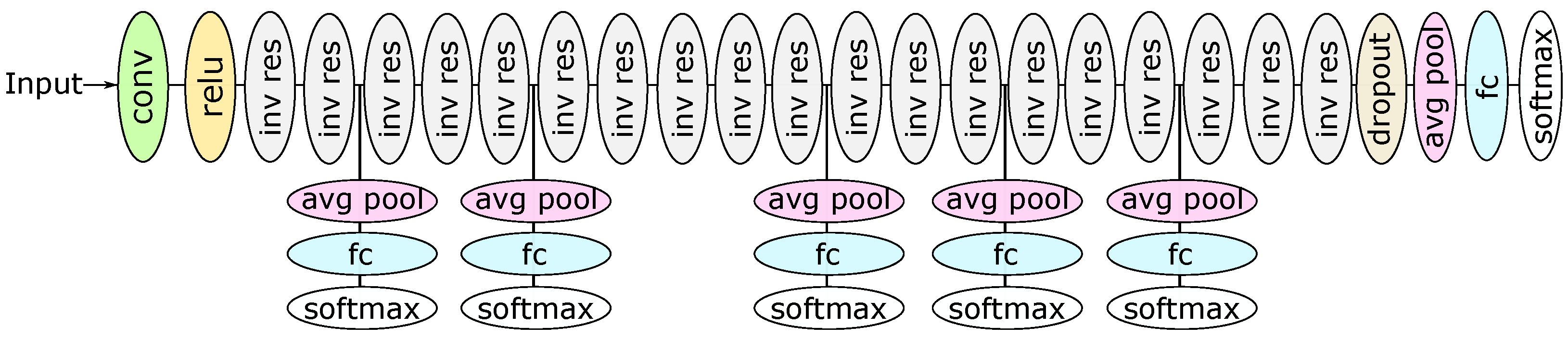
This work considers a Convolutional Neural Network (CNN), a DNN type widely employed in computer vision. More specifically, we employ a MobileNetV2 [12] model using the Caltech-256 image recognition dataset [13]. First, we add side branches to MobileNetV2, investigating how the number of side branches affects the chances of classifying the image at the edge, when varying the confidence threshold. Next, we perform experiments using Amazon EC2 instances to check how these choices affect inference time. Using a real edge-based scenario, we show that employing an early-exit DNN can reduce the inference time by approximately 27% to 61% compared to a cloud-only processing scenario. In this last one, the cloud processes all DNN layers. Moreover, we show that the confidence threshold configuration plays a key role to determine the inference time. Therefore, adjusting this threshold is vital to balance inference time and classification confidence. Finally, we show that inserting side branches indiscriminately saturates the number of images classified on them, serving only to introduce processing delay.

The remainder of this article is organized as follows. Section 2 reviews the related work. Section 3 briefly reviews convolutional neural networks and early-exit DNNs, discussing our design choices and the DNN architecture with part of the layers at the edge and part of the layers at the cloud. Next, Section 4 presents the methodology used to analyze early-exit DNNs in an edge-based scenario. Section 5 discusses the experimental results, emphasizing the impact on the overall system performance of different parameters. Section 6 evaluates the early-exit DNNs in a real edge-based scenario and demonstrates that employing early-exit DNNs can reduce inference time. Finally, Section 7 concludes this work and presents future research directions.

2. Related Work

Cloud-based and edge-computing-based solutions create contrasting challenges for applications deployed at the network edge [14,15]. In mobile scenarios, on the one hand, cloud computing becomes dependent on network conditions, which can be an obstacle to applications with low latency requirements. On the other hand, edge devices can introduce computing delays because of hardware limitations compared with the cloud. Several approaches to accelerate DNN inference at the edge devices, including a hardware-based approach that uses hardware implementation to tackle this issue [16]. For example, Eyeriss v2 [17] designs an accelerator for DNNs on mobile devices, while Karras et al. [18] employ an FPGA board to accelerate DNN inference. However, this paper focuses on tackling the DNN inference acceleration using DNN partitioning.

DNN partitioning determines which DNN’s layers must be processed at the network edge and which layers can be processed at the cloud. As such, Kang et al. propose the Neurosurgeon system, which builds a predictive model to determine layer-wise inference times at the edge and the cloud [19]. Neurosurgeon performs an exhaustive search to determine which partitioning scheme minimizes inference time. In a different approach, Hu et al. propose DADS (Dynamic Adaptive DNN Surgery), a system that models DNNs as graphs and handles DNN partitioning as a minimum cut problem [20]. Both works strive to minimize the inference time by finding the appropriate partitioning scheme, but they do not focus on the model performance.

Unlike previous works, Pacheco and Couto approach optimal early-exit DNN partitioning between edge devices and the cloud to minimize inference time [21]. To handle that, the authors model early-exits DNNs and possible partitioning decisions as a graph. Then, they use the graph to solve the partitioning problem as a shortest path problem. Their work employs a well-known CNN called AlexNet [22]. In another work, Pacheco et al. propose early-exit DNNs with expert side branches to make inference more robust against image distortion [23]. To this end, they propose expert side branches trained on images with a particular distortion type. In an edge computing scenario with DNN partitioning, they show that this proposal can increases the estimated accuracy of distorted images on edge, improving the offloading decisions. Both works focus on decision-making aspects of early-exits, having a different focus than the present work. Hence, they do not perform a sensibility analysis, considering the impact of the number of side branches and the confidence threshold. Laskaridis et al. considers the confidence threshold in their study, but with a fixed number of side branches [11].

Passalis et al. use the concept of feature vectors to leverage the relationship between the vector content learned from previous side branches to predict samples at the deeper layers of the DNN [24]. Their proposal is evaluated using five different datasets and implementing a hierarchical chain of side branches. They achieve superior performance when compared to independent early-exit implementations. However, despite their contribution to aggregation methods, i.e., methods that use information learned from previous side branches, the learning model is not generalized to low latency applications. This occurs because the results computed by a side branch must finish before the computation performed by the deeper layers can take place.

Early-exit DNNs have been deployed in different scenarios. In industrial settings, for instance, it is possible to observe multiple applications. Li et al. implement DeepIns to minimize latency on industrial process inspection tasks [25]. Their system leverages the concept of early-exit DNNs directly. Nevertheless, the hardware limitations of industrial edge devices are far less expressive than other IoT-based scenarios. Furthermore, DeepIns does not evaluate the use of multiple early-exits inside the local network or even at the edge device. Instead, the authors try to optimize the system performance by using a single decision point. At this possible exit point, the data can be directly inferred or sent to the cloud.

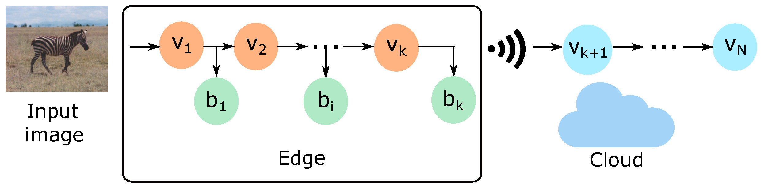
Finally, in the same way as [11,21,23], we consider early-exit DNNs employed in an adaptive offloading scenario with DNN partitioning. In this case, an early-exit DNN model is split into two parts. One part is processed at the edge, while the second is processed at the cloud server. Unlike the previous works, we analyze how much early-exit DNNs can reduce the inference time to make feasible latency-sensitive applications.

3. Early-Exit Neural Networks at the Network Edge

Recent developments on DNNs have proved their applicability for several computer vision tasks, such as image classification and object detection. Many of these modern computer vision applications demand high responsiveness [26], i.e., they require DNN inference to be performed as quickly as possible. In autonomous driving, for instance, this requirement is around 300 ms [27]. In a cognitive assistance application, the maximum latency tolerated can be as low as 100 ms [28]. Hence, alternatives to accelerate inference tasks can be considered as enablers of low latency applications. This is indeed the role of early-exit DNNs at the network edge.

3.1. CNNs in a Nutshell

Before we address early-exit DNNs, a quick review of neural networks (NN) is appropriate. Neural networks are versatile machine learning tools that can adapt to data with little or no preprocessing [29]. They are constructed in a layer-wise fashion, with each layer having a number of computational units, known as neurons. Each neuron receives a number of inputs, which are combined and applied to a nonlinear function. These neurons connect with each other. The weights of these connections determine the computation to be performed once the NN is trained. To derive more complex models, it is common to construct NNs with multiple layers. These deeper models are referred to as DNNs.

A common DNN realization is to make neuron connections to subsequent layers. NNs of this type are called feedforward, as the data flows through the layers in a single direction from the input to the output layer, meaning that there are no cycles. One of the simplest feedforward implementations employs fully connected layers, in which each neuron connects with all the neurons of the next layer. It is possible to construct a more suited layer for processing well-structured data, such as images [30]. We can achieve this by making the connections more localized. Hence, each neuron connects with the closest neurons in the DNN architecture and share the weights across each of these groups of connections. This layer is called a convolutional layer, as this group of connections forms a set of weights, known as a convolutional filter, that slides across the data [2].

3.2. Early-Exit DNNs

Features extracted at shallower layers, i.e., layers closer to the DNN input layer, can be rich enough to classify part of the samples from a dataset [9,11,24]. Early-exit DNNs exploit this fact by processing these features in an early attempt to perform predictions. By using this mechanism, some samples can be predicted without being processed by the entire DNN, which can greatly reduce the inference time. To enable this approach, early-exit DNNs must have side branches positioned at intermediate layers. Figure 1 illustrates a generic early-exit DNN architecture. In this figure, the grey vertices, labeled as $v_i$, represent the layers of the main neural network, called the DNN backbone, while the red vertices $b_i$ represent the side branches, also called side branches. These side branches enable early sample classification if the prediction confidence is above some predetermined confidence threshold.

In this paper, we follow the procedure proposed by BranchyNet for early-exit DNN training [9]. Once trained, early-exit DNNs can receive an input image for object classification. This input image is processed, layer-by-layer, until it reaches the i-th side branch $b_i$. On the side branch, the data goes through a set of fully connected layers producing an output vector, which we denote by ${\mathit{z}}_i$. Then, the early-exit DNN computes a probability vector ${\mathit{p}}_i=\mathrm{softmax}\left({\mathit{z}}_i\right)\propto exp\left({\mathit{z}}_i\right)$, where each vector element corresponds to the probability that the object is of a particular class.

Next, for each input image, we can obtain the classification confidence as $max{\mathit{p}}_i$ and verify if the confidence is greater than or equal to a given confidence threshold $p_{\mathrm{tar}}$. If so, the i-th side branch can classify the image as follows $\widehat{y}=arg\; max\left({\mathit{p}}_i\right)$, where $\widehat{y}$ corresponds to the inferred class. In this case, the DNN inference terminates, and no further data processing is required throughout the remaining DNN layers. In this case, early classification can reduce the inference time. However, suppose the confidence value is less than $p_{\mathrm{tar}}$. In that case, the input image must continue throughout the remaining DNN backbone layers until it reaches the next side branch, where the same procedure is repeated. If none of the side branches produces confidence greater than or equal to $p_{\mathrm{tar}}$, the image is processed by the remaining DNN backbone layers until it reaches the output layer. This layer thus generates a probability vector and computes the classification confidence. Suppose this confidence value provided by the DNN backbone’s output layer does not reach $p_{\mathrm{tar}}$. In that case, the classification chooses the class with the highest confidence value among all side branches and the output layer of the backbone [11,23].

This paper analyzes early-exit DNNs employed in an adaptive offloading scenario, as illustrated in Figure 2. This scenario considers that the early-exit DNN is divided into two parts. The first corresponds to the DNN layers with side branches (i.e., $v_1$ to $v_k$, and also $b_k$), which are positioned at the edge device. The second part, composed of the remaining DNN layers ($v_{k+1}$ to $v_N$), is implemented at a cloud server.

In adaptive offloading, the early-exit DNN inference works as follows for an image classification task. Firstly, the edge receives the input image from the end-user and runs the early-exit DNN inference, following the procedure described before. In this scenario, if any side branches placed at the edge reach $p_{\mathrm{tar}}$ value, the image is classified, terminating the inference at the edge. Otherwise, if no side branches reach $p_{\mathrm{tar}}$, the edge offloads the DNN inference to the cloud, which executes the remaining DNN backbone layers. This increases the inference time due to the communication delay associated with the data transfer. Therefore, less complex images are likely to be processed at the network edge in this scenario, while more complex and challenging images are offloaded to the cloud. Hence, edge offloading can be considered adaptive as the decision of transferring an image to the cloud depends on the complexity to provide a confident classification [31].

Pacheco et al. show that early-exits DNN, including its side branches, can be overconfident about their predictions, providing unreliable offloading decisions [31]. Moreover, they show that applying a temperature scaling calibration method [32] allows more reliable predictions, improving edge offloading decisions. Thus, after training the early-exit DNN, we also employ temperature scaling to calibrate side branches of the early-exit DNN model. To this end, we follow the methodology proposed in [31].

4. Methodology

In this section, we detail the CNN architecture and the dataset used in our experiments. This work uses MobileNetV2 [12] as the DNN backbone. MobileNetV2 is a Convolutional Neural Network (CNN) optimized for low latency applications, Figure 3 presents MobileNetV2’s architecture. It is constructed in such a manner that it needs significantly less computation when compared to a standard CNN [33]. We then introduce multiple side equidistantly-positioned branches, dividing the DNN into segments with the same number of FLOPS (Floating Point Operations). The number of side branches is an additional hyperparameter of early-exit DNNs. The literature has already addressed this strategy to place side branches [11,23].

Table 1. MobileNetV2’s architecture.

Layer	Input	Output	n
Conv	224 × 224 × 3	112 × 112 × 32	1
ReLU6	112 × 112 × 32	112 × 112 × 32	1
Inverted Residual	112 × 112 × 32	56 × 56 × 24	2
Inverted Residual	56 × 56 × 24	28 × 28 × 32	3
Inverted Residual	28 × 28 × 32	14 × 14 × 64	4
Inverted Residual	14 × 14 × 64	14 × 14 × 96	3
Inverted Residual	14 × 14 × 96	7 × 7 × 160	3
Inverted Residual	7 × 7 × 160	7 × 7 × 320	1
Conv	7 × 7 × 320	7 × 7 × 1280	1
ReLU6	7 × 7 × 1280	7 × 7 × 1280	1
AvgPool 7 × 7	7 × 7 × 1280	1 × 1 × 1280	1
Fully-connected	1 × 1 × 1280	258	1

details MobileNetV2’s architecture, presenting the input and output shape in each DNN layer. Each line in this table presents a layer or a module of layers, repeated n times.

We construct architectures from two up to five side branches using a pre-trained MobileNetV2. We use the parameter weights of this pre-trained DNN as an initial solution. After that, we train the DNN with the side branches. While the training process is used primarily to train the parameters of the side branches, it also tunes the weights of the DNN backbone. This ensures that the side branches can work effectively with the DNN backbone, as the layers to which the side branches are attached are also adjusted for the early classification task. Upon training termination, each model is saved to be used in the testing step.

In the test step, we measure the number of samples that are prematurely classified. We consider that an early classification occurs when a sample exits a side branch exceeding a confidence threshold, which we denote by $p_{\mathrm{tar}}$. Firstly, different $p_{\mathrm{tar}}$ values are tested. In this paper, we vary $p_{\mathrm{tar}}$ from 0.7 to 0.9 with a step of 0.05.

A high $p_{\mathrm{tar}}$ value represents more rigorous criteria, classifying fewer images earlier at side branches. Therefore, we can vary this confidence threshold and measure the tradeoff between relaxing this criterion and the occurrence of early classification. Once the layers up to the last branch are kept at the edge, with the remainder of the DNN stored at the cloud, the data is offloaded to the cloud whenever an image is not classified early. Ideally, we would desire that the side branches classify almost all images since it could bring latency down significantly. However, if we choose a relatively low $p_{\mathrm{tar}}$, the classification performance could reach a point where the inferences obtained are unreliable. The source code developed for this work is available at an open repository [34].

This work considers an image recognition dataset called Caltech-256 [13]. The Caltech-256 dataset is composed of high-quality images tailored for object detection applications. This dataset has 256 classes of ordinary objects, such as motorbikes and shoes, and one clutter class, totaling 257 classes. Each class has at least 80 samples. We divide the dataset into 80% images for training, 10% for validation, and 10% for testing.

5. Early-Exit Hyperparameter Analysis

This section aims to evaluate the early-exit mechanism, taking an in-depth look at the tradeoff between inference time and classification performance. We then investigate the impact of including side branches on the volume of data transferred to the cloud. We can estimate the volume of data processed locally by measuring the number of samples classified at the side branches. It is worth mentioning that whenever a classification is performed at a side branch, the edge does not send the corresponding sample to the cloud for further processing. In addition, given that $p_{\mathrm{tar}}$ decides whether a sample needs to go further in the backbone DNN, we also need to investigate the impact of this parameter on the number of samples classified at each side branch. It is possible to evaluate if adding a side branch at certain positions is beneficial or not.

Early-exit DNNs aim to reduce the overall inference time, defined as the time required to classify an input image. Hence, the analyzed system is considered successful if the average time spent in the early-exit DNN model does not exceed the time spent transmitting the data to a cloud server. However, it is expected that a sample exiting the DNN backbone achieves a better classification score than it would receive exiting at a side branch. In our experiments, this tradeoff is tackled by quantifying the amount of time spent with local computations. This time is upper bounded by the time needed for data transmission to the cloud and receiving the response back on edge. Using early exits is only valid if the possible confidence penalty is compensated by a lower inference time.

5.1. Inference Probability

We start by evaluating the probability of performing inference at the edge device for multiple early-exit configurations. To this end, we train an early-exit DNN with different numbers of side branches. We train the early-exit DNN as follows. First, we replace the output layer of the DNN backbone with a new one whose number of neurons corresponds to the number of classes in the dataset. In this case, the output layer of the DNN backbone has 258 neurons, as shown in Table 1. The hyperparameters used in training are available in our repository [34]. We train the early-exit DNN model until the validation loss stops decreasing for five epochs in a row. Inference probability is defined as the number of images classified at the side branches, implemented at the edge, divided by the total number of images in the test dataset for a given confidence threshold $p_{\mathrm{tar}}$. To evaluate this inference probability, we fix the $p_{\mathrm{tar}}$ value and the number of side branches positioned at the edge. Then, we can compute the inference probability, counting the number of images from the test dataset classified on the edge device. Next, we repeat this procedure by varying the number of branches at the edge device and the $p_{\mathrm{tar}}$ value.

Figure 4 shows the probabilities of performing inference on the edge device for multiple early-exit configurations. We train each scenario with a fixed number of side branches. Note that this fixed number varies from two, Figure 4a, to five, Figure 4d. The curves on each figure were generated by “activating” only the corresponding number of side branches at a time. Each curve is labeled with a number n. This number indicates that the first n side branches are activated for the experiment. For example, Figure 4c considers an early-exit DNN trained with four side branches. Hence, the curve labeled as 2 indicates a situation where only the first two side branches are activated. In the same way, the curve labeled as 4 indicate the activation of all side branches for that DNN. Consequently, we measure the proportion of samples on the test set classified up to that branch while varying the confidence threshold. The yellow curve on Figure 4c shows that close to 40% of all samples were classified up to the third side branch, while the green curve shows that close to 80% of all samples were classified up to the fourth side branch, which includes samples classified by the third side branch.

It is immediately noticeable in Figure 4 that side branches positioned very close to the input layer are less beneficial. To confirm this statement, note that the probability of inferring samples up to the first branch is approximately zero for all DNNs. On the other hand, the side branches positioned in deeper layers can anticipate the classification of a considerable portion of samples at the edge. This behavior is expected since the features distilled by the shallowest DNN layers, i.e., closest to the input layer, are more similar to the raw inputs, instead of the desired feature maps at the deepest parts of the DNN, i.e., closest to the output layer. Moreover, these results show that adding side branches allows classifying samples at the edge while avoiding performing DNN inference at the cloud. Thus, the early-exit mechanism can be useful for several applications that could transfer network traffic to the cloud, either for data privacy reasons or to reduce inference time.

Finally, we can also observe that adding side branches saturate the proportion of samples classified sooner at the edge. This can be seen comparing Figure 4c,d, where the addition of a fifth side branch, which is slightly closer to the output of the DNN, does not result in a much higher inference probability at the edge device.Therefore, an appropriate number of side branches provides reduced inference time without wasting computational resources.

In summary, this section has shown that early-exit DNNs employed in an adaptive offloading scenario can indeed classify a considerable portion of samples at the edge. It can be beneficial to reduce the inference time and also the network traffic to the cloud. Next, we analyze the classification confidence provided by the side branches in early-exit DNNs.

5.2. Classification Confidence

This section investigates the impact of side branches positioning along the early-exit DNN architecture on the classification confidence. The confidence can be a fair estimate for accuracy in a calibrated DNN [31,32]. Consequently, this section also evaluates how side branch placement impacts early-exit DNN performance. To this end, this experiment performs early-exit DNN inference on all images from the test set. We collect the classification confidence at the branch that classified the image for each of these images. Then, we compute the mean classification confidence with confidence intervals of 95%. We repeat this experiment for each confidence threshold $p_{\mathrm{tar}}$ and number of side branches in early-exit DNN model, as described in the previous section. For this experiment, all branches are activated. For example, using the reasoning of Section 5.1, we consider only $n=4$ for a DNN with four side branches and $n=5$ for a DNN with five side branches.

Figure 5 presents the mean classification confidence for multiple early-exit configurations. Each curve represents the mean confidence of the samples classified on a given branch. By examining Figure 5, it becomes evident that increasing the $p_{\mathrm{tar}}$ value required for images to be classified at the side branches also increases the mean confidence of the classified images on a branch. It is true since a high threshold makes the branch accept only samples with high confidence. Consequently, the branch classifies fewer samples as we increase the threshold, as shown in Figure 4. Additionally, we can also observe that the results for the first branch present a high variability (i.e., confidence interval). This happens because, as shown in Figure 4, this branch classifies nearly zero images. As the variability is related to the number of experimental samples, it gets high when the number of classified images is low on a given branch.

Figure 5 also shows that side branches closer to the output layer provide more confident classifications than the shallower side branches. Considering confidence as a suitable estimate for accuracy, we can state that deeper branches tend to achieve better performance. In this regard, Figure 5c,d present missing data points for an early-exit DNN with only the first side branch. In these figures, missing points indicate that no samples are classified at that particular $p_{\mathrm{tar}}$ value. This behavior occurs because the first side branch is placed too close to the input layer so that the features extracted by the DNN backbone layers up to this side branch do not make it possible to reach $p_{\mathrm{tar}}$. Thus, according to Figure 5c,d, the first side branch can be removed since this branch cannot classify any images for more rigorous $p_{\mathrm{tar}}$ values. Furthermore, according to Figure 4, this side branch classifies a negligible amount of images, which is another reason to remove it.

Figure 5c shows that the third branch provides a slight gain in confidence compared to the second side branch. On the other hand, Figure 5d shows that the fourth side branch also has a slight gain in confidence compared to the third one. Therefore, in Figure 5d, we can state that the third and the fourth side branches are redundant, so that we can remove one of them. On the one hand, since the confidence gain between the third and the fourth side branch is negligible, we can remove the fourth side branch to save processing time. On the other hand, Figure 4d has shown that the fourth side branch can classify far more images than the third one. In this case, it is more advantageous to remove the third side branch. Thus, removing one of the side branches must balance the extra processing time to run the deepest side branch and the number of early classifications that it can provide.

5.3. Processing Time

The processing time at the edge device depends on the choice of early-exit positioning and the value of $p_{\mathrm{tar}}$. Using the test set, we evaluate the processing time considering an edge equipped with an Intel i5-9600K CPU with six cores at 3.70 GHz and an NVIDIA GeForce RTX 2080 Ti GPU. This machine runs a Debian 9.13 operating system. We employ the DNN with five branches from Section 5.2, with $p_{\mathrm{tar}}=0.8$. For this evaluation, we place all DNN layers at the edge, and thus there is no cloud offloading. We measure the time required to process each image of the test set. Figure 6a shows the processing time for each branch, where the sixth branch is the backbone’s exit. The processing time for a side branch is the mean of all images that were classified in that side branch. While not easily visible in the figure, we also plot the confidence interval of 95%. Figure 6a shows the impact of traversing the DNN in the processing time. For example, an image takes almost twice the time to go to branch three compared to a classification on branch two.

Figure 6b shows the mean processing time of the test set images as a function of the confidence threshold $p_{\mathrm{tar}}$. For this experiment, we consider the same DNN used in Figure 6a. We thus evaluate the processing time of each classification and plot the mean and confidence interval of 95%. This figure shows that increasing $p_{\mathrm{tar}}$ also increases the processing time at the edge device. Consequently, we must choose $p_{\mathrm{tar}}$ carefully to balance the performance gains by classifying some samples at the edge device, while not introducing unnecessary delays in the form of processing time at the edge.

In a nutshell, determining what is considered a correct classification impacts the amount of data that needs to travel further down the backbone DNN by adopting stricter rules, i.e., higher $p_{\mathrm{tar}}$ values, fewer data exits at the side branches closer to the input layer. It directly impacts the processing time since requiring more confident classifications also requires more data processing throughout the DNN. Figure 6b reflects the processing time increase with the exiting threshold, where the higher the $p_{\mathrm{tar}}$ value, the more confidence we have in the sample classified at each side branch.

6. Real Scenario Experiments

This section evaluates the inference time considering the adaptive offloading scenario presented in Figure 2. Hence, the edge and the cloud work collaboratively to perform early-exit DNN inference for image classification tasks. The inference time is defined as the time needed to complete a DNN inference (i.e., to infer the class corresponding to an input image) after the reception of an image. If the input is classified on a side branch, this is the time needed to run the inference at the edge entirely. Otherwise, the inference time is the sum of the processing time and networking time. The first one is the time to process the DNN layer on the edge and on the cloud. The second one is the time to send the image from the edge to the cloud plus the time to send the DNN output to the edge.

The experiment employs a local server as edge and an Amazon EC2 virtual machine as the cloud server to emulate a real edge computing application. The edge and the cloud server are developed using Python Flask 2.0.1, and they communicate using the HTTP protocol. The edge server emulates the role of an end device or even an intermediate one, such as an access point on a radio base station. On the one hand, the edge server is the same one as employed in Section 5.3, located in Rio de Janeiro, Brazil. On the other hand, the cloud server is an Amazon EC2 g4dn.xlarge instance running Ubuntu 20.04 LTS. This cloud server is equipped with four vCPUs from an Intel Cascade Lake CPU and an NVIDIA Tesla T4 GPU. For this experiment, the cloud server is located in São Paulo (i.e., sa-east-1 AWS region), also in Brazil, approximately 430 km away from Rio de Janeiro. We chose this location because it is the closest AWS region to our edge, which would be a consistent choice in a real latency-sensitive application. In this experiment, we implement a MobileNetV2 model with five side branches as our early-exit DNN. 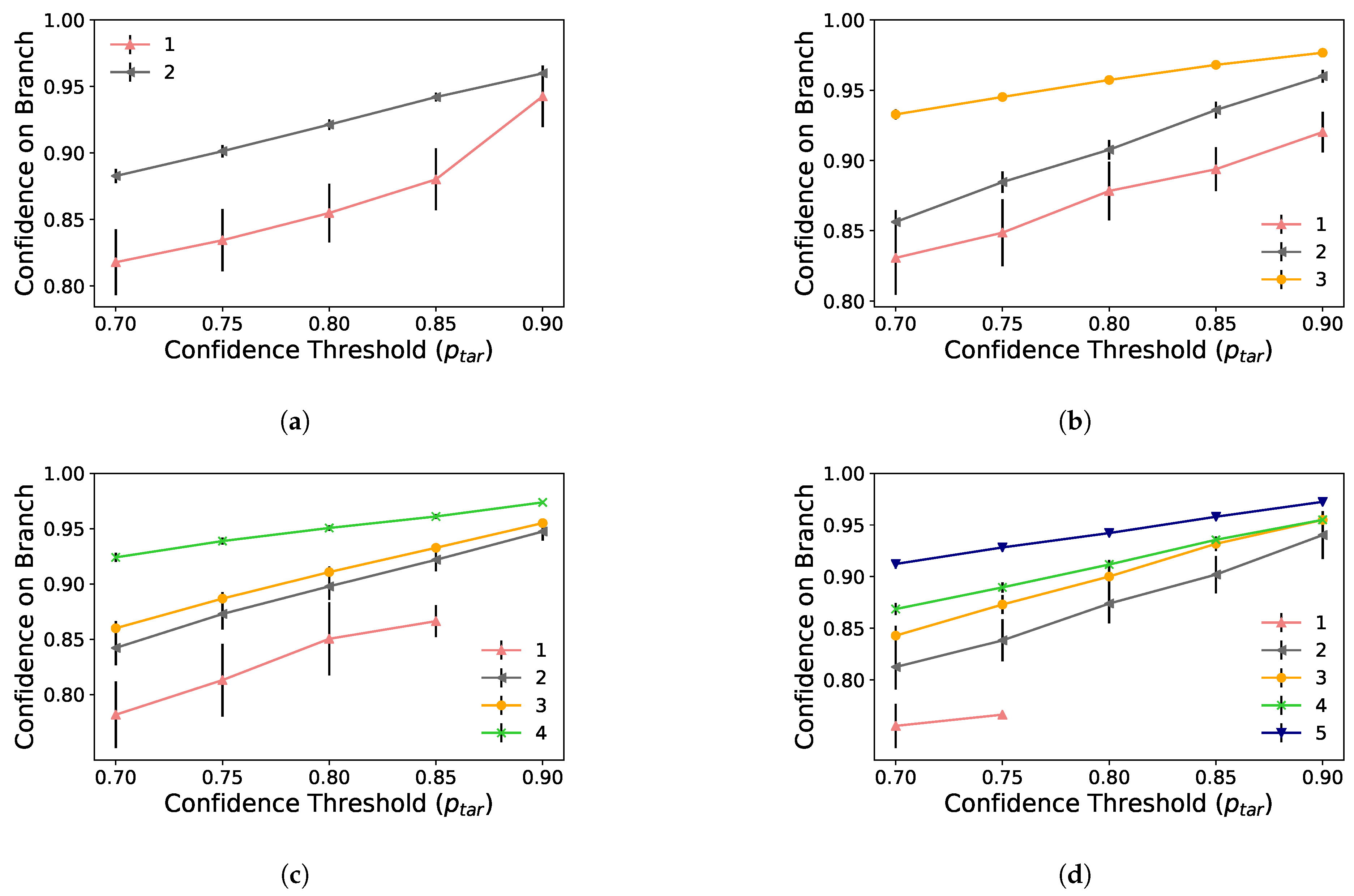However, as shown in Figure 4, the first and second side branches cannot classify a considerable portion of the images from the test set. Thus, these side branches only introduce processing delay. To solve it, we remove these first two side branches in this analysis.

Additionally, we also implement a cloud-only processing scenario, in which the cloud processes all neural layers of a regular DNN (i.e., without side branches). This scenario works as a performance baseline for our adaptive offloading scenario under analysis. In the cloud-only scenario, we implement a regular MobileNetV2 for the sake of consistent comparison.

Before running the experiment, we evaluate the network conditions between the edge server and the Amazon EC2 instance. To this end, we measure the throughput and RTT (Round-Trip Time) between the edge server and the cloud instance using, respectively, iPerf3 and ping. In this case, the measured throughput and RTT are 94 Mbps and 12.8 ms, respectively. It is important to emphasize that these values only illustrate the network conditions since they may change during the experiment.

For each image from the test set, the edge server starts a timer to measure the inference time and run the early-exit DNN inference, as described in Section 3. If any of the side branches implemented at the edge can reach the confidence threshold $p_{\mathrm{tar}}$, the inference terminates earlier at the edge, finishing the timer. Otherwise, the edge server sends the intermediate results to the cloud server, which processes the remaining DNN layers. In this case, the edge server waits for the HTTP response from the cloud to finish the inference timer. In contrast, in the cloud-only processing scenario, the experiment starts a timer to measure the inference time and send the image directly to the cloud server, which runs the DNN inference. Then, the edge waits for an HTTP response from the cloud to finish the inference timer. These procedures are run for each image from the test set, for each $p_{\mathrm{tar}}$ value, and for each number of side branches at the edge. For each setting, we compute the mean inference time with confidence intervals of 95%.

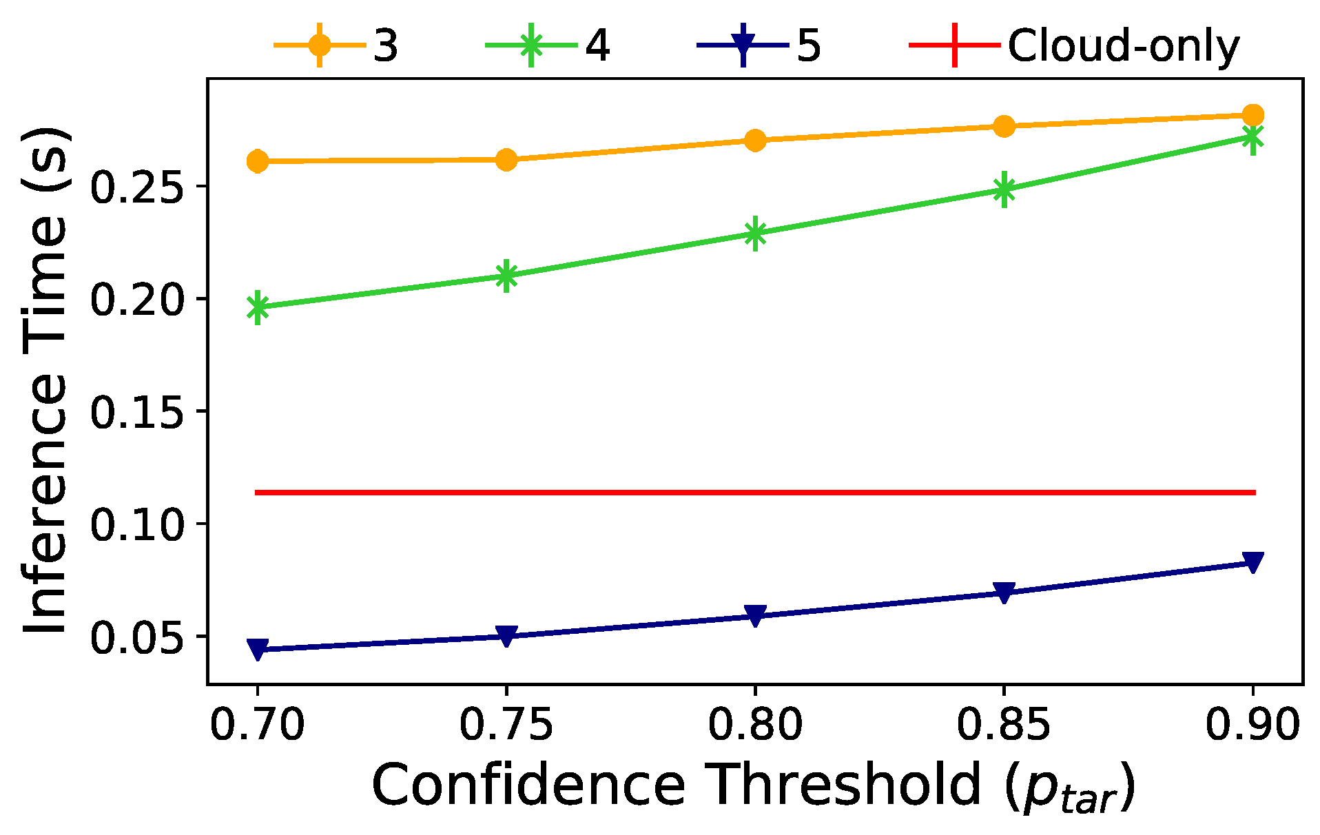
Figure 7 presents the inference time results according to the $p_{\mathrm{tar}}$ value configuration. Each curve in this figure is the inference time result for an early-exit DNN with a different number of side branches at the edge, using the same reasoning of Section 5.1. However, branches one and two are always deactivated. For example, the yellow curve shows the inference time considering that the DNN has only the third branch at the edge, while the green curve shows a DNN with the third and fourth branches. In contrast, the red line represents the cloud-only processing scenario, which serves as a performance baseline. At first glance, we can notice that the inference time increases as we set $p_{\mathrm{tar}}$ to higher values. This behavior occurs because a higher $p_{\mathrm{tar}}$ value reduces the probability of performing inference at the edge. Hence, the edge sends more images to the cloud, introducing network delay more often. The cloud-only curve is constant since its DNN in independent of $p_{\mathrm{tar}}$.

We can instantly observe the benefit of adding side branches by looking at the blue curve, which reduces inference time by using five side branches. Notably, the additional processing time at the edge device must provide enough gain to justify not sending the data to the cloud to reduce overall inference time. Additionally, we show that there is a tendency for the early-exit DNN to increase overall inference time with a high enough confidence threshold. Therefore, $p_{\mathrm{tar}}$, which is already application-dependent, must be carefully selected to minimize inference time while satisfying possible Service Level Agreements (SLAs). For example, we can highlight that the DNN with five side branches at the edge meets the 0.1 s latency requirement, which is required for a cognitive assistance application [28].

At this stage, we have demonstrated that, in an adaptive offloading scenario, the early-exit DNN can significantly reduce the inference time and outperform the cloud-only processing scenario. Moreover, our results show that the early-exit DNN model represents a fundamental approach for meeting the requirements of latency-sensitive applications.

7. Conclusions and Future Scope

This work has shown that early-exit DNNs can classify a significant amount of images earlier at side branches. Thus, in an adaptive offloading scenario, this corresponds to classifying most samples at the edge, avoiding sending unnecessary data to the cloud. Next, we have demonstrated experimentally that this early-exit mechanism can reduce inference time by outperforming the cloud-only processing scenario. In fact, the results have shown that early-exit DNNs can meet the latency requirements of sensitive applications.

In terms of early-exit DNN design, we have shown that inserting side branches closer to the input DNN layer is not worthwhile. This is true since only a negligible amount of samples are classified into these branches. Therefore, these shallow side branches only introduce processing delay. On the other hand, we have demonstrated that the deeper side branches, i.e., those closer to the output layer, provide more confident classification, reaching the confidence threshold more often. Hence, these side branches can classify more images at the edge. Thus, it is more advantageous to insert side branches at the deeper layers. Regarding the confidence threshold, this work showed that the choice of this threshold value considerably impacts the number of samples classified at the edge, and consequently, the inference time. However, the selection of the confidence threshold is application-driven since it depends on the desired DNN accuracy and inference time. Regarding the number of side branches, it is important to emphasize that inserting side branches adds processing delay. Therefore, the processing delay caused by the insertion of the side branches cannot be greater than so high that it is not advantageous to process in the edge device.

We will expand our inference time analysis in future steps considering a three-tier architecture composed of an end device, intermediate device, and the cloud server. Additionally, we intend to explore the prospect of integrating an FPGA environment to leverage its low latency capabilities. Finally, we plan to employ a resource-constrained device as the edge device, such as a Raspberry Pi. Finally, we will also evaluate other DNN models using different datasets for image classification.

References

1. Ioannidou, A.; Chatzilari, E.; Nikolopoulos, S.; Kompatsiaris, I. Deep Learning Advances in Computer Vision with 3D Data: A Survey. ACM Comput. Surv. 2017, 50, 1–38. [Google Scholar] [CrossRef]
2. Bochie, K.; Gilbert, M.S.; Gantert, L.; Barbosa, M.S.M.; Medeiros, D.S.V.; Campista, M.E.M. A Survey on Deep Learning for Challenged Networks: Applications and Trends. J. Netw. Comput. Appl. 2021, 194, 103213. [Google Scholar] [CrossRef]
3. Kuutti, S.; Bowden, R.; Jin, Y.; Barber, P.; Fallah, S. A Survey of Deep Learning Applications to Autonomous Vehicle Control. IEEE Trans. Intell. Transp. Syst. 2021, 22, 712–733. [Google Scholar] [CrossRef]
4. Sze, V.; Chen, Y.H.; Yang, T.J.; Emer, J.S. Efficient Processing of Deep Neural Networks: A Tutorial and Survey. Proc. IEEE 2017, 105, 2295–2329. [Google Scholar] [CrossRef] [Green Version]
5. Son, Y.; Jeong, J.; Lee, Y. An Adaptive Offloading Method for an IoT-Cloud Converged Virtual Machine System Using a Hybrid Deep Neural Network. Sustainability 2018, 10, 3955. [Google Scholar] [CrossRef] [Green Version]
6. Baccarelli, E.; Scarpiniti, M.; Momenzadeh, A.; Ahrabi, S.S. Learning-in-the-Fog (LiFo): Deep Learning Meets Fog Computing for the Minimum-Energy Distributed Early-Exit of Inference in Delay-Critical IoT Realms. IEEE Access 2021, 9, 25716–25757. [Google Scholar] [CrossRef]
7. Kocić, J.; Jovičić, N.; Drndarević, V. An End-to-End Deep Neural Network for Autonomous Driving Designed for Embedded Automotive Platforms. Sensors 2019, 19, 2064. [Google Scholar] [CrossRef] [Green Version]
8. Miotto, R.; Wang, F.; Wang, S.; Jiang, X.; Dudley, J.T. Deep learning for healthcare: Review, opportunities and challenges. Brief. Bioinform. 2017, 19, 1236–1246. [Google Scholar] [CrossRef]
9. Teerapittayanon, S.; McDanel, B.; Kung, H.T. BranchyNet: Fast inference via early exiting from deep neural networks. In Proceedings of the 2016 23rd International Conference on Pattern Recognition (ICPR), Cancun, Mexico, 4–8 December 2016; pp. 2464–2469. [Google Scholar] [CrossRef] [Green Version]
10. Scardapane, S.; Scarpiniti, M.; Baccarelli, E.; Uncini, A. Why Should We Add Early Exits to Neural Networks? Cogn. Comput. 2020, 12, 954–966. [Google Scholar] [CrossRef]
11. Laskaridis, S.; Venieris, S.I.; Almeida, M.; Leontiadis, I.; Lane, N.D. SPINN: Synergistic Progressive Inference of Neural Networks over Device and Cloud. In Proceedings of the 26th Annual International Conference on Mobile Computing and Networking (MobiCom’20), London, UK, 21–25 September 2020; Association for Computing Machinery: New York, NY, USA, 2020. [Google Scholar] [CrossRef]
12. Sandler, M.; Howard, A.G.; Zhu, M.; Zhmoginov, A.; Chen, L. Inverted Residuals and Linear Bottlenecks: Mobile Networks for Classification, Detection and Segmentation. arXiv 2018, arXiv:1801.04381. [Google Scholar]
13. Griffin, G.; Holub, A.; Perona, P. Caltech-256 Object Category Dataset; CalTech Report; California Institute of Technology: Pasadena, CA, USA, 2007. [Google Scholar]
14. Hobfeld, T.; Schatz, R.; Varela, M.; Timmerer, C. Challenges of QoE management for cloud applications. IEEE Commun. Mag. 2012, 50, 28–36. [Google Scholar] [CrossRef]
15. Ahmed, E.; Rehmani, M.H. Mobile Edge Computing: Opportunities, solutions, and challenges. Future Gener. Comput. Syst. 2017, 70, 59–63. [Google Scholar] [CrossRef]
16. Ngo, D.; Lee, S.; Ngo, T.M.; Lee, G.D.; Kang, B. Visibility Restoration: A Systematic Review and Meta-Analysis. Sensors 2021, 21, 2625. [Google Scholar] [CrossRef]
17. Chen, Y.H.; Yang, T.J.; Emer, J.; Sze, V. Eyeriss v2: A flexible accelerator for emerging deep neural networks on mobile devices. IEEE J. Emerg. Sel. Top. Circuits Syst. 2019, 9, 292–308. [Google Scholar] [CrossRef] [Green Version]
18. Karras, K.; Pallis, E.; Mastorakis, G.; Nikoloudakis, Y.; Batalla, J.M.; Mavromoustakis, C.X.; Markakis, E. A hardware acceleration platform for AI-based inference at the edge. Circuits Syst. Signal Process. 2020, 39, 1059–1070. [Google Scholar] [CrossRef]
19. Kang, Y.; Hauswald, J.; Gao, C.; Rovinski, A.; Mudge, T.; Mars, J.; Tang, L. Neurosurgeon: Collaborative intelligence between the cloud and mobile edge. ACM Comput. Archit. News (SIGARCH) 2017, 45, 615–629. [Google Scholar] [CrossRef] [Green Version]
20. Hu, C.; Bao, W.; Wang, D.; Liu, F. Dynamic Adaptive DNN Surgery for Inference Acceleration on the Edge. In Proceedings of the IEEE Conference on Computer Communications (INFOCOM), Paris, France, 29 April–2 May 2019; pp. 1423–1431. [Google Scholar]
21. Pacheco, R.G.; Couto, R.S. Inference Time Optimization Using BranchyNet Partitioning. In Proceedings of the 2020 IEEE Symposium on Computers and Communications (ISCC), Rennes, France, 7–10 July 2020. [Google Scholar] [CrossRef]
22. Krizhevsky, A.; Sutskever, I.; Hinton, G.E. Imagenet classification with deep convolutional neural networks. Adv. Neural Inf. Process. Syst. 2012, 25, 1097–1105. [Google Scholar] [CrossRef]
23. Pacheco, R.G.; Oliveira, F.D.V.R.; Couto, R.S. Early-exit deep neural networks for distorted images: Providing an efficient edge offloading. In Proceedings of the IEEE Global Communications Conference (GLOBECOM), Madrid, Spain, 7–11 December 2021; pp. 1–6, Accepted for publication. [Google Scholar]
24. Passalis, N.; Raitoharju, J.; Tefas, A.; Gabbouj, M. Efficient adaptive inference for deep convolutional neural networks using hierarchical early exits. Pattern Recognit. 2020, 105, 107346. [Google Scholar] [CrossRef]
25. Li, L.; Ota, K.; Dong, M. Deep Learning for Smart Industry: Efficient Manufacture Inspection System With Fog Computing. IEEE Trans. Ind. Inform. 2018, 14, 4665–4673. [Google Scholar] [CrossRef] [Green Version]
26. Satyanarayanan, M. The emergence of edge computing. Computer 2017, 50, 30–39. [Google Scholar] [CrossRef]
27. Hobert, L.; Festag, A.; Llatser, I.; Altomare, L.; Visintainer, F.; Kovacs, A. Enhancements of V2X communication in support of cooperative autonomous driving. IEEE Commun. Mag. 2015, 53, 64–70. [Google Scholar] [CrossRef]
28. Chen, Z.; Hu, W.; Wang, J.; Zhao, S.; Amos, B.; Wu, G.; Ha, K.; Elgazzar, K.; Pillai, P.; Klatzky, R.; et al. An empirical study of latency in an emerging class of edge computing applications for wearable cognitive assistance. In Proceedings of the Second ACM/IEEE Symposium on Edge Computing, San Jose, CA, USA, 12–14 October 2017; p. 14. [Google Scholar]
29. LeCun, Y.; Bengio, Y.; Hinton, G. Deep learning. Nature 2015, 521, 436–444. [Google Scholar] [CrossRef] [PubMed]
30. LeCun, Y.; Bengio, Y. Convolutional networks for images, speech, and time series. Handb. Brain Theory Neural Netw. 1995, 3361, 1995. [Google Scholar]
31. Pacheco, R.G.; Couto, R.S.; Simeone, O. Calibration-Aided Edge Inference Offloading via Adaptive Model Partitioning of Deep Neural Networks. In Proceedings of the ICC 2021—IEEE International Conference on Communications, Montreal, QC, USA, 14–23 June 2021; pp. 1–6. [Google Scholar]
32. Guo, C.; Pleiss, G.; Sun, Y.; Weinberger, K.Q. On calibration of modern neural networks. In Proceedings of the 34th International Conference on Machine Learning, Sydney, Australia, 6–11 August 2017; pp. 1321–1330. [Google Scholar]
33. Howard, A.G.; Zhu, M.; Chen, B.; Kalenichenko, D.; Wang, W.; Weyand, T.; Andreetto, M.; Adam, H. MobileNets: Efficient convolutional neural networks for mobile vision applications. arXiv 2017, arXiv:1704.04861. [Google Scholar]
34. Pacheco, R.G.; Bochie, K.; Gilbert, M.S.; Couto, R.S.; Campista, M.E.M. Available online: https://github.com/pachecobeto95/early_exit_dnn_analysis (accessed on 8 October 2021).
Figure 1. Generic representation of an early-exit DNN.
Information 12 00431 g001
Figure 2. Adaptive edge offloading using early-exit DNNs. Adapted from the paper [23].
Information 12 00431 g002
Figure 3. MobileNetV2’s architecture consists of a convolutional (conv) and Rectified Linear Unit (ReLU) layers, followed by 19 inverted residual (inv res) layers. The data is then passed through a dropout layer and an average pooling (avg pool) layer. Finally, a fully connected (fc) layer and a softmax layer are used to perform classification. The side branches are then introduced in the indicated positions.
Information 12 00431 g003
Figure 4. Probability of performing inference on the device for multiple early-exit configurations. (a) MobileNetV2 trained with 2 side branches. (b) MobileNetV2 trained with 3 side branches. (c) MobileNetV2 trained with 4 side branches. (d) MobileNetV2 trained with 5 side branches.
Information 12 00431 g004
Figure 5. Mean inference confidence for each side branch across different early-exit configurations. Missing data points indicate that no samples were classified at that particular side branch. (a) MobileNetV2 trained with 2 side branches. (b) MobileNetV2 trained with 3 side branches. (c) MobileNetV2 trained with 4 side branches. (d) MobileNetV2 trained with 5 side branches.
Information 12 00431 g005
Figure 6. Processing time without cloud offloading. (a) Overall processing time in each branch. (b) Overall processing time as a function of the inference threshold p tar .
Information 12 00431 g006
Figure 7. Overall inference time in a real edge-based scenario as a function of the confidence threshold p tar .
Information 12 00431 g007