Article

Double Deep Autoencoder for Heterogeneous Distributed Clustering

1
Department of Business Administration, Chung Yuan Christian University, Taoyuan 32023, Taiwan
2
Department of Computer Science and Information Management, Soochow University, Taipei 10048, Taiwan
*
Author to whom correspondence should be addressed.
Information 2019, 10(4), 144; https://doi.org/10.3390/info10040144
Submission received: 4 March 2019 / Revised: 15 April 2019 / Accepted: 15 April 2019 / Published: 17 April 2019
(This article belongs to the Section Artificial Intelligence)

Abstract

:
Given the issues relating to big data and privacy-preserving challenges, distributed data mining (DDM) has received much attention recently. Here, we focus on the clustering problem of distributed environments. Several distributed clustering algorithms have been proposed to solve this problem, however, previous studies have mainly considered homogeneous data. In this paper, we develop a double deep autoencoder structure for clustering in distributed and heterogeneous datasets. Three datasets are used to demonstrate the proposed algorithms, and show their usefulness according to the consistent accuracy index.

1. Introduction

Knowledge discovery in database (KDD) processing involves transforming raw data into interesting information and knowledge, and has been a popular issue in the fields of machine learning and data mining (DM). Traditional DM focuses on mining information from a central dataset; in contrast, the issues of big data and preserving privacy highlight the need for distributed data mining (DDM). DDM concentrates on retrieving knowledge from distributed datasets that may be homogeneous or heterogeneous [1,2], instead of joining or merging these datasets into a central dataset.
This characteristic distinguishes DDM from DM, and results in the traditional DM methods being unable to deal with big or privacy-preserving data, because these data are stored by being distributed. Here, we propose a new algorithm for the clustering task in distributed environments.
One of the main tasks in KDD is clustering, which involves grouping similar data together and is the first step of exploring unknown data. Generally, typical clustering algorithms can be divided into hierarchical, centroid-based, and density-based methods. By calculating the similarity between data points, a data point can be assigned to a cluster, and the data points within a cluster are similar with respect to their attributes. However, when a big dataset is considered, some clustering methods, such as hierarchical and spectral clustering methods, may suffer from the problem of feasibility because of their huge complexity. This can be illustrated by O( N 2 ), where N is the number of data points [3]. Hence, Steinbach et al. [4] and Beil et al. [5] proposed modified algorithms to deal with large and high-dimensional data. However, these methods are mainly limited to a central database, rather than a distributed dataset.
To consider handling distributed datasets for the clustering problem, we should propose distributed clustering methods and they should be divided into horizontal and vertical methods, or homogeneous and heterogeneous distributed clustering algorithms, with respect to the type of dataset. Most distributed clustering algorithms are homogeneous algorithms, including those of [6,7] and are an extension of parallel computing. On the other hand, [8] first proposed the collective hierarchical clustering (CHC) algorithm to consider the distributed clustering problem in heterogeneous databases. Later on, several papers on heterogeneous distributed clustering algorithms, such as those by [9,10,11], were proposed to consider more complex situations [12].
Usually, heterogeneous databases can use principle component analysis (PCA) and correlation analysis to reduce the number of dimensions and consider the interactive relations between features in past research [13]. However, as PCA and correlation analysis do not consider nonlinear representative or nonlinear interactive relations between features, they might lose some important information for clustering. Hence, in this paper, instead of using PCA, we consider the double deep autoencoder model for the above issues, as follows: the stage of the replica neural network learns the nonlinear codes from each local dataset. Then, we concatenate all local codes to be the input of the server neural network, to learn the nonlinear global codes across the replicas; that is, the interactive relationships between the features. We use the double deep autoencoder and distinguish the proposed method from others.
In this paper, we define our problem as follows. Assume k parties, P 1 , , P k , own large private datasets, D 1 , , D k . They want to apply a clustering algorithm to the whole dataset without simply joining all datasets, due to a big data issue or privacy-preserving reason. Hence, the information that a party can use is the model output of other parties. Note that no trusted party is considered here. In addition, we consider a heterogeneous view of the datasets, which is that all parties hold exclusive information about the features of all the records. To overcome this problem, we developed a double deep autoencoder to extract the nonlinear important features by considering the information from the self and other parties. Compared with past papers, the original contribution of this paper is the integration of the deep autoencoders, and clustering with the concept of deep learning. Three heterogeneous distributed datasets are used to demonstrate the proposed algorithms and the ability to overcome our problem. Therefore, the contribution of this paper is the proposal of a new deep learning model, specifically the double deep autoencoder, to deal with distributed and homogeneous datasets.
The rest of this paper is organized as follows: the distributed clustering algorithm is introduced in Section 2. The proposed double deep autoencoder used in the distributed environment is presented in Section 3. Experiments are given in Section 4, and the last section presents the discussion and conclusion.

2. Distributed Clustering Algorithms

The distributed clustering processes can be depicted as shown in Figure 1. Each local dataset, i.e., a partition of a whole dataset, is used to perform local clustering, e.g., k-means. Then, the global representation is gathered from each local clustering and perform global clustering. Finally, the result of the global clustering is used to apply the local datasets to evaluate the result of the distributed clustering algorithm. Distributed clustering algorithms enable the clustering problem to be solved under a distributed environment.
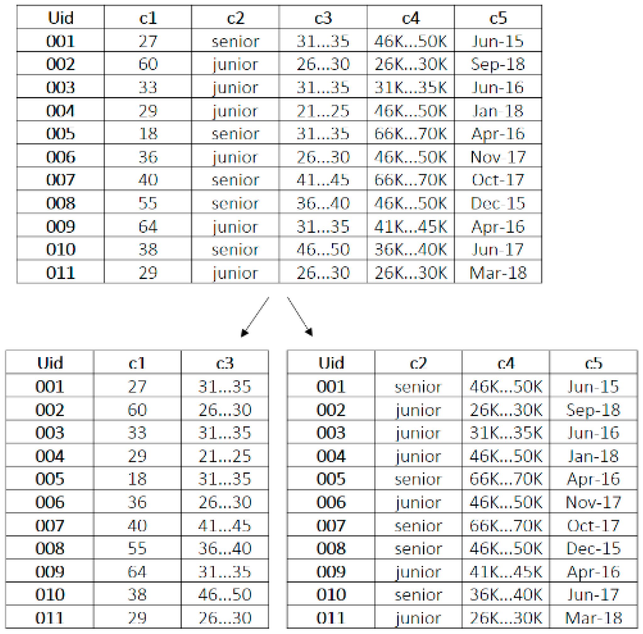
The property of local datasets is divided into horizontally distributed (homogeneous) and vertically distributed (heterogeneous) datasets. In the former, all databases across distributed data sites share the same set of attributes. In the latter, the attributes differ among the distributed datasets in a heterogeneous situation. For example, a heterogeneous dataset is divided by a central dataset, as shown in Figure 2.
Most DDM algorithms use the concept of parallel computing and algorithms to consider the homogeneous dataset situation [14,15]. On the other hand, some algorithms, such as those of [16,17], generate local data and transmit them to a central coordinator, which then performs the clustering algorithm. In addition, some researchers have focused on fuzzy datasets, e.g., the PFCM-c* algorithm [18], IFDFC algorithm [19], and parallel fuzzy c-means algorithm [20]. Although these methods have been proposed to deal with various problems in distributed environments, these algorithms only work in homogeneous databases that all share the same attributes.
In order to deal with the problem of the heterogeneous datasets in the distributed environment, Kargupta and his colleagues extended the concept of CHC to propose a distributed hierarchal clustering [8,9]. However, it may suffer from problems of computational time and memory in a big or high-dimensional dataset, similar to conventional hierarchical clustering algorithms. Hence, Kargupta et al. [9] proposed a dimensionality reduction of CHC to solve the problem of the computation complexity. However, this method disregards the possible interaction effects among attributes in different datasets, and forgoes some levels of information in the data. Moreover, it cannot deal with categorical data with the conventional principal component analysis. Although other distributed clustering algorithms for heterogeneous datasets are proposed, e.g., OPTICS algorithm [21] and the SDBDC algorithm [17], these methods assume clusters of similar density, and may have problems separating nearby clusters [22] and the appropriate choice of parameters, such as the radius parameter, which is still an open issue [23]. In sum, none of the existing algorithms adequately address the problems we have outlined here.

3. Double Deep Autoencoder

Deep learning has recently received much attention because of its successful applications in practice and academia, and many types of deep neural networks have been proposed, such as convolutional neural networks [24,25], recurrent neural networks [26], and deep autoencoders [27]. The purpose of deep learning is to construct many hidden layers (usually more than two hidden layers) to capture and extract complicated information from data in supervised and unsupervised models. In this paper, we will use one kind of deep learning model—the deep autoencoder—to develop distributed clustering algorithms which avoid the previously presented problems of [9]’s OPTICS and SDBDC algorithms.

3.1. Deep Autoencoder

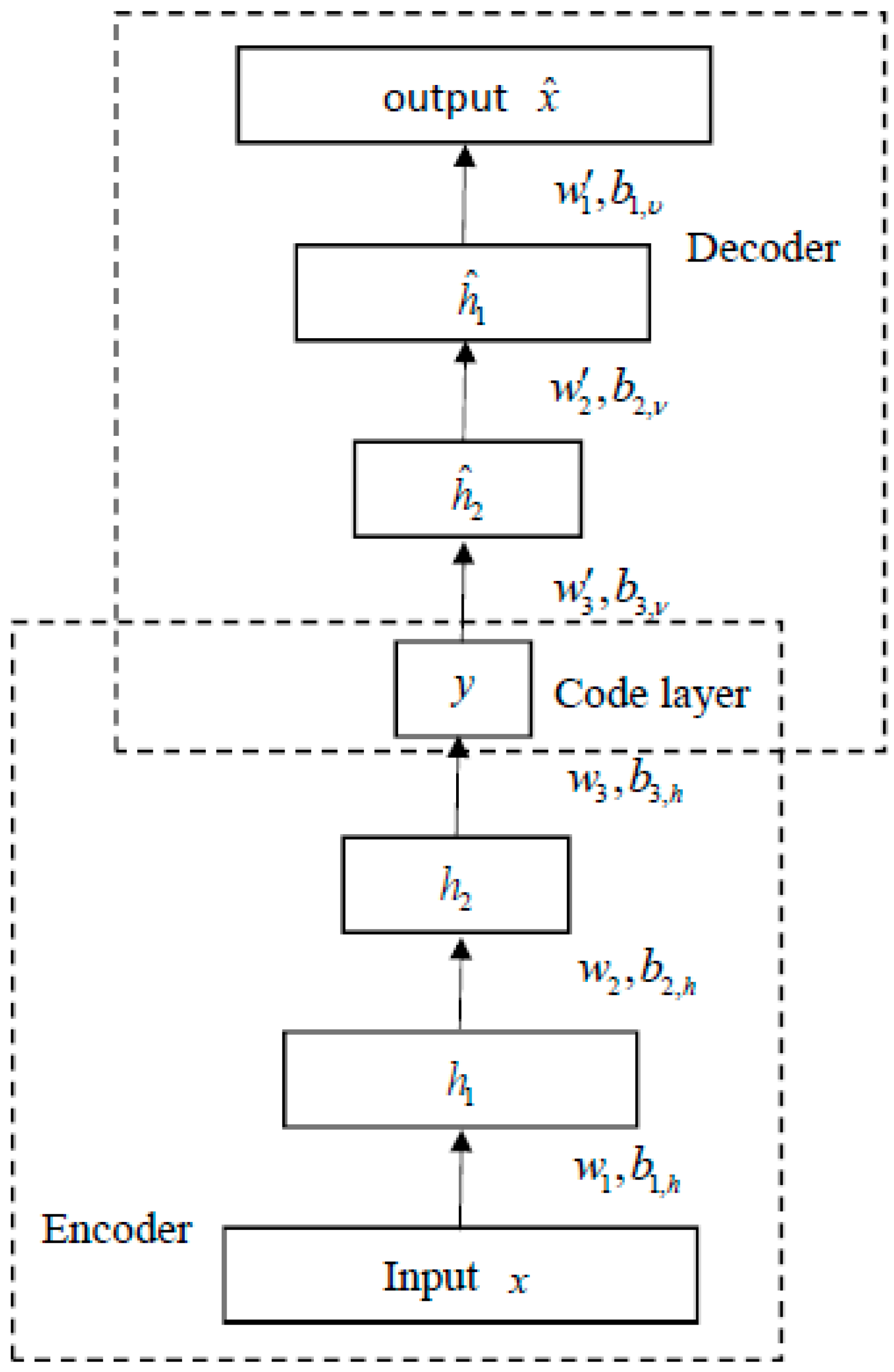
The structure of the deep autoencoder was originally proposed by [28], to reduce the dimensionality of data within a neural network. They proposed a multiple-layer encoder and decoder network structure, as shown in Figure 3, which was shown to outperform the traditional PCA and latent semantic analysis (LSA) in deriving the code layer.
Later, several modified autoencoders, such as the stacked sparse autoencoder (SSAE) [29] and stacked similarity-aware Autoencoder [30], were proposed.
If one hidden layer is considered, the optimization process of finding weights in the autoencoder can be viewed as minimizing the following loss objective:
J ( x , x ^ ) = | | x x ^ | | 2 = | | x σ ( W ( σ ( W x + b ) ) + b ) | | 2
where x is the input, x ^ is the output, σ ( W x + b ) denotes the code or latent variables, and W and b are the weight matrix and bias vector, respectively, for the encoder and satisfy the condition W W = 1 , where W and b , respectively, are the weight and bias parameters for the decoder, indicating the relationship between the encoder and decoder. We can add more hidden layers to naturally extend the original autoencoder under the deep structure model, and to consider a more complicated and nonlinear representation of variables.
Deep autoencoders have been widely used in pre-trained deep neural networks, such as in coevolution neural networks (CNNs) and recurrent neural networks (RNNs), and reported as a useful way to represent the original variables. In addition, deep autoencoders have been successfully used in the fields of speech recognition [31], 3D shape retrieval [32], face recognition [33,34,35], and more. Next, we introduce the proposed algorithm.

3.2. Replica Neural Network

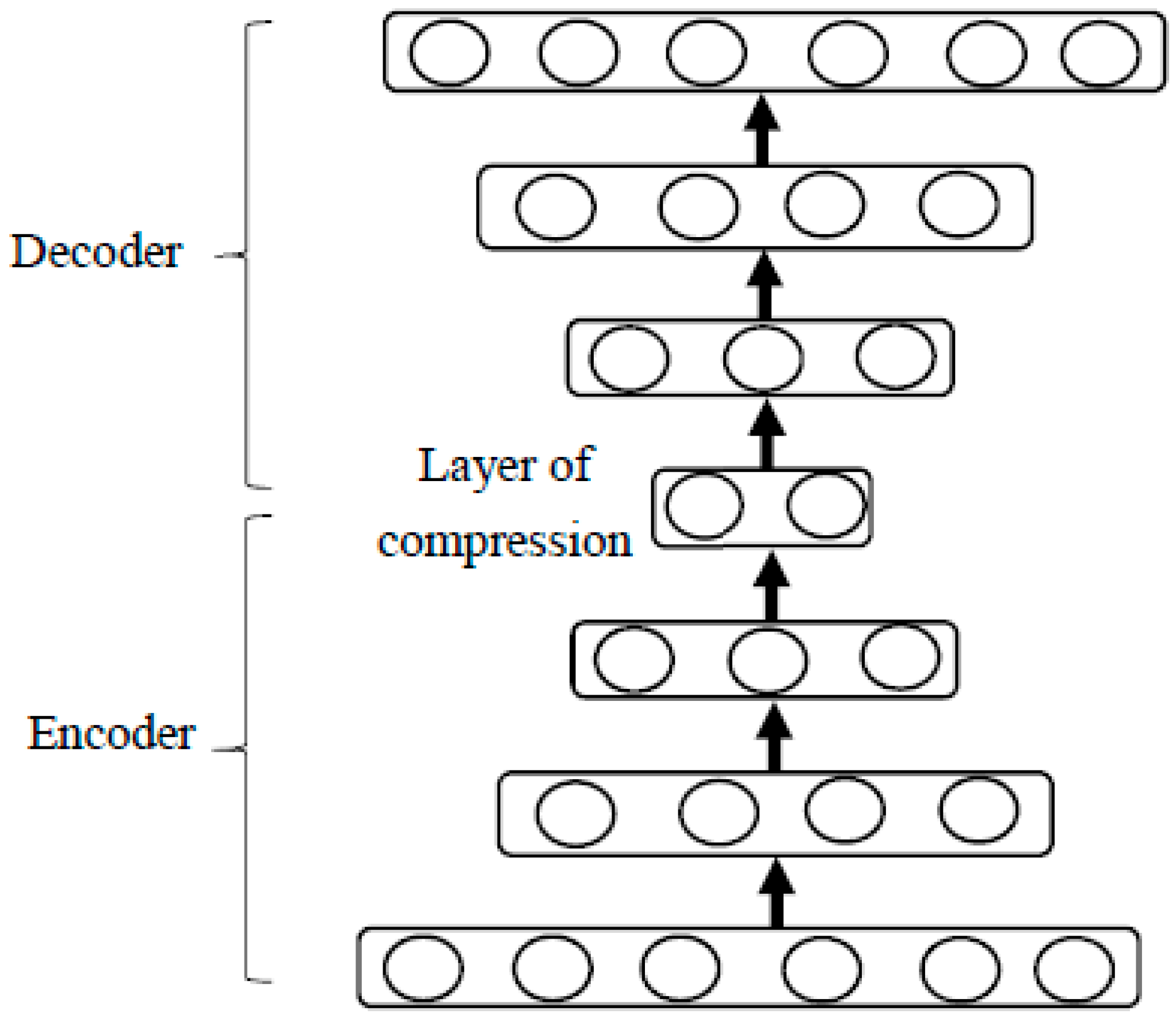
In the local database, we design a deep autoencoder that contains multiple encoder and decode layers, as shown in Figure 4.
The layer of compression is initially used in the bottle-neck scheme in the autoencoder, and is a compressed feature vector designed to represent and capture the information of input features and significantly reduce the dimensions of the features. The usefulness of the code layer has been identified as the increase of the accuracy of models, and is widely used in deep learning algorithms [36]. In addition, in the practical usage of the deep autoencoder, the number of hidden neurons may exceed the number of input variables. The purpose is to map the input variables for the hyperdimensional feature spaces to the segment data more effectively. Here, we input our heterogeneous and distributed datasets into different replicas. Note that the heterogeneous and distributed datasets mean each replica holds the partial and exclusive features of the whole dataset. Then, the codes of all replicas will be concatenated together to be the input layer of the server neural network.

3.3. Server Neural Network

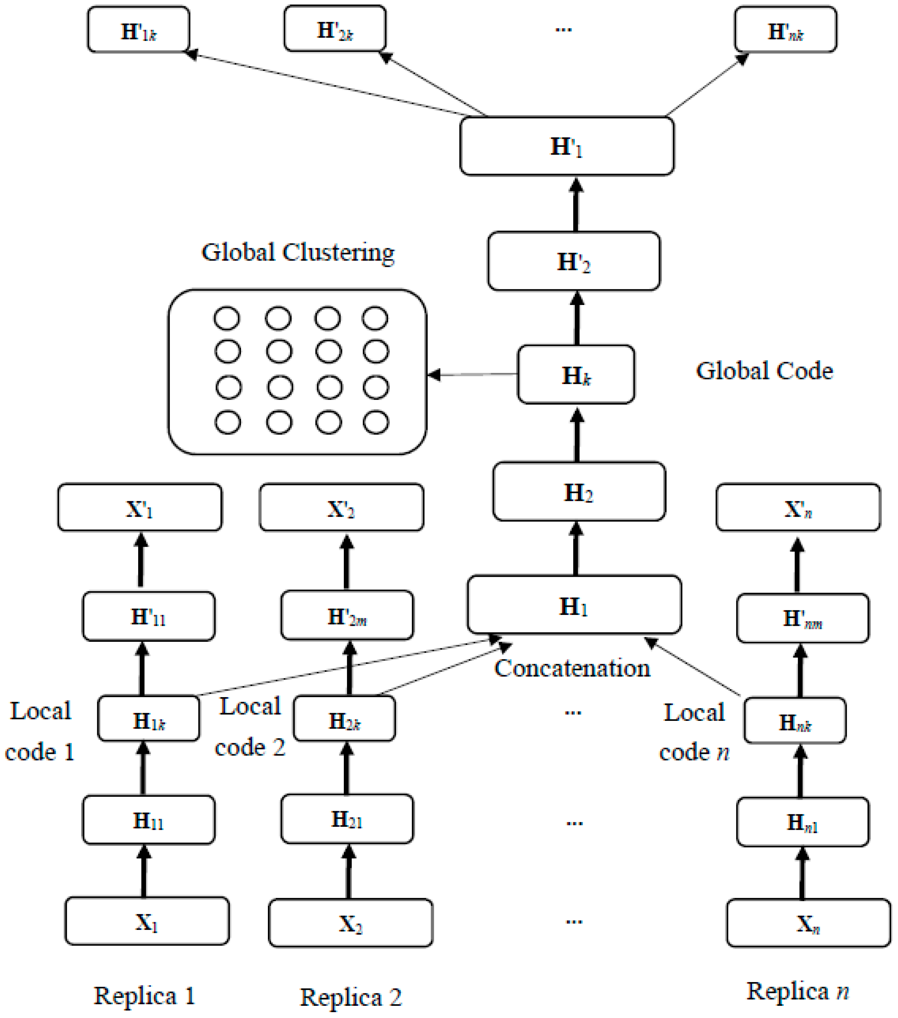
Next, we should consider multiple local datasets to derive the global clustering result under the structure of the deep autoencoder in a distributed environment. The arrangement is described as follows. First, assume there are n distributed local datasets and each local dataset processes the deep autoencoder simultaneously to capture the compressed information of the features by the layer of compression (code). Then, we concatenate all local codes as the input features of the global deep autoencoder. Furthermore, the global code is trained to represent the information of the local codes. Finally, the global code of the global deep autoencoder is used to obtain the global results of the clustering algorithms. Note that we use k-means, self-organizing maps (SOM), and spectral clustering algorithms here to compare the results of our experiments. The proposed structure of the global deep autoencoder is presented in Figure 5.
We should highlight that the purpose of H1 in the server is to combine the information of all replicas so that the global code can extract the information and learn the interaction effect among the distributed features. In addition, since all Hik are dimensionally reduced, we can avoid the problem of high dimensions in combining all local codes. Then, we can use the global code layer to obtain the global result of the clustering by processing another deep autoencoder.
Finally, we can formulate the local and global objectives of the proposed model, respectively, as:
J ( X i , X i ) = | | X i X i | | 2 , i = 1 , , n
and
J ( c o n c a t ( H j k ) , H j k ) = | | c o n c a t ( H j k ) H j k | | 2 , j = 1 , , n
where X i denotes the input matrix of the ith replica, X i denotes the reconstructed output of the ith replica, H j k denotes the local code of the jth replica, c o n c a t ( ) denotes the concatenate function, c o n c a t ( H j k ) is the global input matrix, and H j k denotes the global reconstructed output.

3.4. Optimization Algorithms

Several optimization algorithms have been proposed to train the above deep autoencoder, including gradient descent and its variants [37]. However, traditional optimization algorithms result in a computational efficiency problem when dealing with a complicated or deep neural network. Hence, the concept of the mini-batch process is considered in which stochastic gradient descent (SGD) is used to take advantage of both the batch and stochastic gradient descents. For simplicity, we use SGD to represent the mini-batch SGD here.
SGD is an iterative method for optimizing a differentiable objective function, and has become one of the most popular first-order optimization methods in the field of machine learning. The training process of updating parameter θ by SGD can be described as:
θ = θ η θ J ( θ ; x ( i : i + k ) ; y ( i : i + k ) )
where θ denotes the gradient, η is the learning rate, and k usually is set to 30–200, where 1 < k < n. From Equation (2), it can be seen that the training samples are randomly selected to process the optimization process, instead of as a whole dataset (as in standard gradient descent), to avoid the problem of computation cost when considering big data. The major advantage of SGD is that it is possible to obtain an unbiased estimate of the gradient by taking the average gradient of a mini-batch of k samples drawn from the data-generating distribution [38]. In addition, we can add the momentum term to accelerate learning [39], and reduce the possible problem of the oscillation by combining the past update along with the current update.
The momentum optimizer can be defined as:
v i ( t + 1 ) α v i ( t ) η θ J ( θ )
θ i ( t + 1 ) θ i ( t ) + v i ( t + 1 )
where α [ 0 , 1 ) denotes the momentum parameter, v i is the velocity of the ith parameter, and η is the learning rate. In addition, the momentum optimizer also solves the poor conditioning of the Hessian matrix and variance in the stochastic gradient. Note that the Hessian matrix is the second order partial derivative of an objective function, and is the major information source of the second-order optimization method.
However, one critical issue of SGD is to determine the appropriate learning rate. Many papers have suggested that the learning rate should be adjusted and regulated by itself, rather than be a constant given by a decision-maker. Hence, many algorithms have been proposed, such as Nesterov, RMSprop, and Adam, to consider adaptive learning rate optimization [40,41,42]. In this paper, we adopt the Nesterov method to determine the learning rate, as given by the following equations:
θ i ( t ) θ i ( t ) + α v i ( t )
v i ( t + 1 ) α v i ( t ) η θ J ( θ i ( t ) )
θ i ( t + 1 ) θ i ( t ) + v i ( t + 1 )
where α [ 0 , 1 ) denotes the momentum parameter, v i is the velocity of the ith parameter, and η is the learning rate.

3.5. Summary of the Proposed Algorithm

The proposed Algorithm 1 can be summarized as the following pseudocode:
Algorithm 1: double deep autoencoder
Input: Replica data samples
  Method:
Replica Neural Networks:
(1)
Load the input x i ,   i = 1 , , n from the ith replica and map the input to the latent representation.
(2)
Apply a reverse mapping to reconstruct the input.
(3)
Map each x i onto its code h i k and its reconstruction x i .
Server Neural Network:
(1)
Concatenate all h i k as the input ( H 1 ) onto its code H k and its reconstruction H 1 by the Nesterov method.
(2)
Process the clustering analysis based on H k .
  Output: Global clustering result.
The proposed algorithm above can be summarized as follow: in replica neural networks, all distributed datasets process the local autoencoders to obtain the local feature space by minimizing the reconstruction error through the optimization algorithm, i.e., the Nesterov method. Then, all local feature spaces are concatenated to form the input of the server neural network to process the global autoencoder to extract the global feature space. Finally, the global feature space is used to run the clustering algorithm, e.g., the k-mean method here, to obtain the final result of the clustering analysis.

3.6. Performance Measurement

The purpose of this paper is to develop a distributed clustering algorithm that can deal with heterogeneous datasets. Hence, the performance of the algorithm should reflect the degree of similarity between the clustering results of the proposed and centralized algorithms. Note that the centralized algorithm means processing data in a central dataset, rather than in distributed datasets. Hence, we proposed the following consistent accuracy index (CAI) to measure the performance of the proposed algorithm:
C A I = i = 1 k j = 1 n j I { m C ( c i j ) m D ( c i j ) } i = 1 k n i
where n i denotes the number of local data; I { 1 , 0 } is the indicator variable, which is equal to one if m C ( c i ) = m D ( c i ) and zero otherwise; and m C ( c i ) and m D ( c i ) are the assigned class calculated by the centralized and distributed clustering algorithms, respectively. Note that CAI = 1 if the clustering results of the centralized and distributed clustering algorithms are the same, and CAI = 0 if the results are totally different.

4. Experiments

Three datasets are used here to demonstrate the proposed algorithm and compute the CAI between centralized and distributed datasets, to demonstrate the efficacy of our method in solving the problem presented here. The first dataset is named Mnist, and contains 70,000 handwritten digits from 0 to 9 with 785 features. The second dataset is called the Covertype dataset, and contains 581,012 instances with 54 features used to predict forest cover type from cartographic variables only. The last dataset, named the Sensorless Drive Diagnosis Dataset (SDDD), contains 58,509 instances with 49 features and is extracted from electric current drive signals. All datasets are provided by the UCI Machine Learning Repository, and the last feature of the datasets is the class variable, which is used as the number of the cluster and is dropped from the training sets.
The description and distributed settings of the datasets are presented in Table 1. For our purposes, we divide the original central dataset into several distributed local datasets according to the number of records. For example, the dataset Mnist is divided into four replicas (subsets), and each replica contains 196 attributes. Hence, we can test the proposed method in different distributed environments. In addition, we randomly select exclusive features to form the local features of each dataset in the first and third datasets. The second datasets split the features based on the data type. The first 10 features are continuous, and the others are dummy variables. Hence, all local datasets contain distinctive features.
The parameters for datasets are arranged as shown in Table 2. In the dataset Mnist, for example, the network structure contains one input and one output with 196 features and seven hidden layers, where 10 is the neuron number of the code for each replica. The hyperbolic tangent function is used as the activation function, the dropout rate is 0.2, and the mini-batch size is 100. In addition, regulation and adaptive learning are used here.
Next, all replicas run the deep autoencoder algorithm for each distributed dataset to obtain the local codes, and then combine them to perform another deep autoencoder algorithm from the server to derive the global code. Finally, the code is used to cluster data points by the k-means, SOM, and spectral algorithms. Note that we use parallel spectral clustering [43] here to deal with the dataset Covertype, since it contains more than 500,000 data points and conventional spectral clustering will result in memory and computational problems when calculating the similarity matrix. The CAI is used to test the performance of the proposed method, and we also use the information of the code to classify data to identify the usefulness of the code. The results of the CAI are presented in Table 3.
From Table 3, it can be seen that the spectral algorithm outperforms the others in terms of the CAI, and the CAI values ranging between 0.75 and 0.81 also indicate the high consistency between the centralized and the proposed clustering results. However, the performance of the DDA+SOM is the worst in this experiment, and shows that the compression features cannot provide essential information for SOM in-clustering.
On the other hand, we can also use the unsupervised clustering accuracy (ACC) [44], as shown in Table 4, to evaluate the average performance of the clustering algorithms with respect to the matching results between predicted labels and ground truth labels.
From the results shown in Table 4, we can see that the spectral algorithm also outperforms the others, with ACC values ranging between 0.60 to 0.74. These values are also competitive with respect to the centralized methods, without losing too much information under the distributed and heterogeneous environments. The results of the ACC values also indicate that SOM has the worst performance, no matter the centralized or distributed situation.
In addition, we also compare the classification accuracy between the centralized and the proposed algorithms. The centralized algorithms use raw data to run the deep autoencoder, and add a softmax layer to predict the classes of the data points. In contrast, we use the global code derived by the DDA algorithm to predict the correct class of the data by adding the softmax layer—also known as the hyperbolic tangent function—here. The centralized and distributed network setting of classification is shown in Table 5.
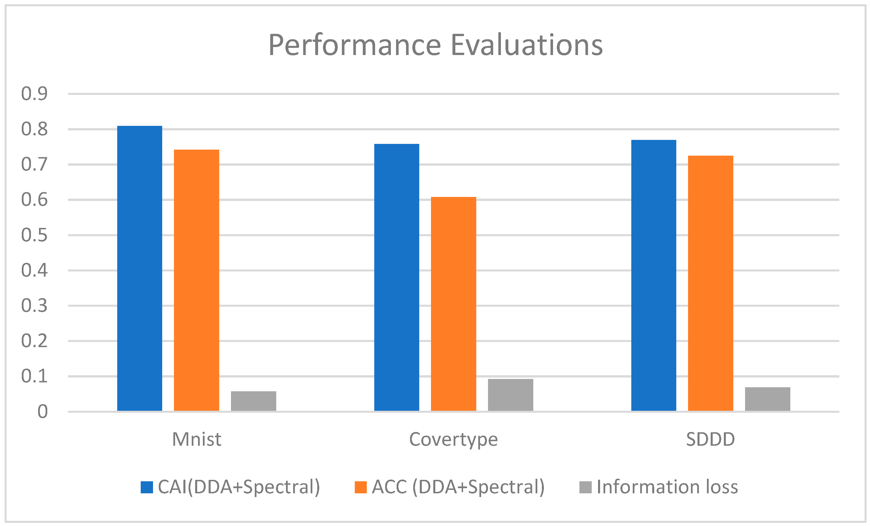
The results of the classification accuracy between centralized and distributed algorithms, as shown in Table 5, also indicate the usefulness of the code to extract and retain the important information between distributed features. In addition, the information loss is only about 5.66% to 9.18%. The best performances of the proposed methods are shown in Figure 6.
Note that the information loss is influenced by the result of the classification based on the experiment results. Hence, more consistent data will perform better with our methods. In sum, these indices show that the accuracy of the proposed method is competitive, even under a distributed environment.

5. Discussion and Conclusions

Although traditional data mining mainly considers handling data in centralized datasets, with the increasing amount of data, centralized storage devices are inadequate for storage of this data. In light of the above issue, distributed databases have been proposed. However, distributed databases complicate the procedures of data mining. In addition, the issue of preserving privacy has also facilitated the emergence of DDM algorithms.
In this paper, we consider a deep learning structure with a double autoencoder setting in local sites and the server, simultaneously. The first deep autoencoder is used to derive the codes for local sites, and the second deep autoencoder is used to derive the global encoder by combining these local encoders. The global encoder should be a good representative for all local features, and achieves this by learning the nonlinear relationships between features. Finally, we can use various kinds of clustering algorithms to obtain global clusters.
The experiment results indicate that DDA and spectral clustering have the highest CAI, between 0.7 and 0.8, compared with k-means and SOM—that is, over 70% of the data points of the central and distributed datasets are assigned to the same clusters. Therefore, we can conclude that DDA can learn the important patterns from the local codes of the intra-datasets. In addition, from the comparisons between accuracy and CAI, it can be inferred that the performance of the CAI is affected by the consistency of the data structure. Therefore, if the data consistency is higher, the value of the CAI becomes higher. Note that the data consistency is reflected in the accuracy of the classification. The higher the accuracy, the higher the data consistency. Furthermore, the results of the ACC and information loss also indicate that the proposed algorithms can account for the clustering analysis under the distributed and heterogeneous environments.
In addition, the empirical results show that the DDA+Spectral algorithm outperforms others in all datasets. Since the input data of the proposed three algorithms are the same, the performance of the algorithms are determined by the ability of the clustering algorithm. In the past research, the performance of the spectral clustering was found to be better than k-means and is consistent with the conclusion here.
The characteristics of the proposed algorithm have the following advantages. First, the local code layers, derived by the deep autoencoder in the replica, can usefully retain the important information of the data and can consider the privacy-preserving issue with fewer features. Second, the mini-batch Nesterov algorithm enables training of the appropriate weights, even with big data. Third, the global code contains all the information of the local codes, and represents them with fewer features. Finally, all centralized algorithms can be embedded in our algorithm to obtain the global clustering results without further modification.

Author Contributions

Writing—original draft, J.-J.H.; Writing—review & editing, C.-Y.C.

Funding

This research received no external funding.

Conflicts of Interest

The authors declare no conflict of interest.

References

  1. Tsoumakas, G.; Vlahavas, I. Distributed data mining. In Database Technologies: Concepts, Methodologies, Tools, and Applications; IGI Global: Hershey, PA, USA, 2009; pp. 157–164. [Google Scholar]
  2. Zeng, L.; Li, L.; Duan, L.; Lu, K.; Shi, Z.; Wang, M.; Wu, W.; Luo, P. Distributed data mining: A survey. Inf. Technol. Manag. 2012, 13, 403–409. [Google Scholar] [CrossRef]
  3. Jain, A.K.; Murty, M.N.; Flynn, P.J. Data clustering: A review. ACM Comput. Surv. 1999, 31, 264–323. [Google Scholar] [CrossRef]
  4. Steinbach, M.; Karypis, G.; Kumar, V. A comparison of document clustering techniques. KDD Workshop Text Min. 2000, 400, 525–526. [Google Scholar]
  5. Beil, F.; Ester, M.; Xu, X. Frequent term-based text clustering. In Proceedings of the Eighth ACM SIGKDD International Conference on Knowledge Discovery and Data Mining, Edmonton, AB, Canada, 23–26 July 2002; p. 436. [Google Scholar]
  6. Ghanem, S.; Kechadi, M.T.; Tari, A.K. New approach for distributed clustering. In Proceedings of the 2011 IEEE International Conference on Spatial Data Mining and Geographical Knowledge Services (ICSDM 2011), Fuzhou, China, 29 June–1 July 2011; pp. 60–65. [Google Scholar]
  7. Ahmad, F.; Chakradhar, S.T.; Raghunathan, A.; Vijaykumar, T.N. Tarazu: Optimizing MapReduce on heterogeneous clusters. In ACM SIGARCH Computer Architecture News; ACM: New York, NY, USA, 2012; p. 61. [Google Scholar]
  8. Johnson, E.L.; Kargupta, H. Collective, Hierarchical Clustering from Distributed, Heterogeneous Data. In Advances in Nonlinear Speech Processing; Springer Nature: Basingstoke, UK, 2000; Volume 1759, pp. 221–244. [Google Scholar]
  9. Kargupta, H.; Huang, W.; Sivakumar, K.; Johnson, E. Distributed Clustering Using Collective Principal Component Analysis. Knowl. Inf. Syst. 2001, 3, 422–448. [Google Scholar] [CrossRef]
  10. Zhai, K.; Boyd-Graber, J.; Asadi, N.; Alkhouja, M.L. Mr. LDA: A flexible large scale topic modeling package using variational inference in mapreduce. In Proceedings of the 21st International Conference on World Wide Web, Lyon, France, 16–20 April 2012; pp. 879–888. [Google Scholar]
  11. Vishalakshi, C.; Singh, B. Effect of developmental temperature stress on fluctuating asymmetry in certain morphological traits in Drosophila ananassae. J. Biol. 2008, 33, 201–208. [Google Scholar] [CrossRef]
  12. Huang, J.-J. Heterogeneous distributed clustering by the fuzzy membership and hierarchical structure. J. Ind. Prod. Eng. 2018, 35, 189–198. [Google Scholar] [CrossRef]
  13. Zhang, J.; Huang, G. Research on distributed heterogeneous data PCA algorithm based on cloud platform. In AIP Conference Proceedings; AIP Publishing: Melville, NY, USA, 2018; Volume 1967, p. 020016. [Google Scholar]
  14. HajHmida, M.B.; Congiusta, A. Parallel, distributed, and grid-based data mining: Algorithms, systems, and applications. In Handbook of Research on Computational Grid Technologies for Life Sciences, Biomedicine, and Healthcare; IGI Global: Hershey, PA, USA, 2012. [Google Scholar]
  15. Roosta, S.H. Parallel Processing and Parallel Algorithms: Theory and Computation; Springer Science & Business Media: Berlin, Germany, 2012. [Google Scholar]
  16. Januzaj, E.; Kriegel, H.P.; Pfeifle, M. Towards effective and efficient distributed clustering. In Proceedings of the Workshop on Clustering Large Data Sets (ICDM2003), Melbourne, FL, USA, 19 November 2003. [Google Scholar]
  17. Januzaj, E.; Kriegel, H.-P.; Pfeifle, M. DBDC: Density Based Distributed Clustering. In Advances in Nonlinear Speech Processing; Springer Nature: Basingstoke, UK, 2004; Volume 2992, pp. 88–105. [Google Scholar]
  18. Coletta, L.F.S.; Vendramin, L.; Hruschka, E.R.; Campello, R.J.G.B.; Pedrycz, W. Collaborative Fuzzy Clustering Algorithms: Some Refinements and Design Guidelines. IEEE Trans. Fuzzy Syst. 2012, 20, 444–462. [Google Scholar] [CrossRef]
  19. Visalakshi, N.K.; Thangavel, K.; Parvathi, R. An Intuitionistic Fuzzy Approach to Distributed Fuzzy Clustering. Int. J. Comput. Theory Eng. 2010, 2, 295–302. [Google Scholar] [CrossRef]
  20. Rahimi, A.; Recht, B. Clustering with normalized cuts is clustering with a hyperplane. Stat. Learn. Comput. Vis. 2004, 56–69. Available online: http://groups.csail.mit.edu/vision/vip/papers/rahimi-ncut.pdf (accessed on 17 April 2019).
  21. Ghesmoune, M.; Lebbah, M.; Azzag, H. Micro-Batching Growing Neural Gas for Clustering Data Streams Using Spark Streaming. Procedia Comput. Sci. 2015, 53, 158–166. [Google Scholar] [CrossRef]
  22. Chowdary, N.S.; Prasanna, D.S.; Sudhakar, P. Evaluating and analyzing clusters in data mining using different algorithms. Int. J. Comput. Sci. Mob. Comput. 2014, 3, 86–99. [Google Scholar]
  23. Achtert, E.; Böhm, C.; Kröger, P. DeLi-Clu: Boosting robustness, completeness, usability, and efficiency of hierarchical clustering by a closest pair ranking. In Pacific-Asia Conference on Knowledge Discovery and Data Mining; Springer: Berlin/Heidelberg, Germany, 2006; pp. 119–128. [Google Scholar]
  24. Abdel-Hamid, O.; Mohamed, A.-R.; Jiang, H.; Deng, L.; Penn, G.; Yu, D. Convolutional Neural Networks for Speech Recognition. IEEE/ACM Trans. Audio Speech Process. 2014, 22, 1533–1545. [Google Scholar] [CrossRef]
  25. Ji, S.; Xu, W.; Yang, M.; Yu, K. 3D Convolutional Neural Networks for Human Action Recognition. IEEE Trans. Anal. Mach. Intell. 2013, 35, 221–231. [Google Scholar] [CrossRef]
  26. Graves, A.; Mohamed, A.-R.; Hinton, G. Speech recognition with deep recurrent neural networks. In Proceedings of the 2013 IEEE International Conference on Acoustics, Speech and Signal Processing, Vancouver, BC, Canada, 26–31 May 2013; pp. 6645–6649. [Google Scholar]
  27. Feng, X.; Zhang, Y.; Glass, J. Speech feature denoising and dereverberation via deep autoencoders for noisy reverberant speech recognition. In Proceedings of the 2014 IEEE International Conference on Acoustics, Speech and Signal Processing (ICASSP), Adelaide, Australia, 4–9 May 2014; pp. 1759–1763. [Google Scholar]
  28. Hinton, G.E.; Salakhutdinov, R.R. Reducing the Dimensionality of Data with Neural Networks. Science 2006, 313, 504–507. [Google Scholar] [CrossRef]
  29. Xu, J.; Xiang, L.; Liu, Q.; Gilmore, H.; Wu, J.; Tang, J.; Madabhushi, A. Stacked sparse autoencoder (SSAE) for nuclei detection on breast cancer histopathology images. IEEE Trans. Med Imaging 2016, 35, 119–130. [Google Scholar] [CrossRef]
  30. Chu, W.; Cai, D. Stacked Similarity-Aware Autoencoders. In Proceedings of the Twenty-Sixth International Joint Conference on Artificial Intelligence (IJCAI-17), Beijing, China, 18–21 June 2017; pp. 1561–1567. [Google Scholar]
  31. Noda, K.; Yamaguchi, Y.; Nakadai, K.; Okuno, H.G.; Ogata, T. Audio-visual speech recognition using deep learning. Appl. Intell. 2015, 42, 722–737. [Google Scholar] [CrossRef]
  32. Zhu, Z.; Wang, X.; Bai, S.; Yao, C.; Bai, X. Deep Learning Representation using Autoencoder for 3D Shape Retrieval. Neurocomputing 2016, 204, 41–50. [Google Scholar] [CrossRef]
  33. Tan, C.C.; Eswaran, C. Reconstruction and recognition of face and digit images using autoencoders. Neural Comput. Appl. 2010, 19, 1069–1079. [Google Scholar] [CrossRef]
  34. Zhang, J.; Hou, Z.; Wu, Z.; Chen, Y.; Li, W. Research of 3D face recognition algorithm based on deep learning stacked denoising autoencoder theory. In Proceedings of the 2016 8th IEEE International Conference on Communication Software and Networks (ICCSN), Beijing, China, 4–6 June 2016; pp. 663–667. [Google Scholar]
  35. Görgel, P.; Simsek, A. Face recognition via Deep Stacked Denoising Sparse Autoencoders (DSDSA). Appl. Math. Comput. 2019, 355, 325–342. [Google Scholar] [CrossRef]
  36. Vincent, P.; Larochelle, H.; Lajoie, I.; Bengio, Y.; Manzagol, P.A. Stacked denoising autoencoders: Learning useful representations in a deep network with a local denoising criterion. J. Mach. Learn. Res. 2010, 11, 3371–3408. [Google Scholar]
  37. Bengio, Y.; Lamblin, P.; Popovici, D.; Larochelle, H. Greedy layer-wise training of deep networks. In Advances in Neural Information Processing Systems; Université de Montréal: Montreal, QC, Canada, 2007; pp. 153–160. [Google Scholar]
  38. Ngiam, J.; Coates, A.; Lahiri, A.; Prochnow, B.; Le, Q.V.; Ng, A.Y. On optimization methods for deep learning. In Proceedings of the 28th International Conference on Machine Learning (ICML-11), Washington, DC, USA, 28 June–2 July 2011; pp. 265–272. [Google Scholar]
  39. Schmidhuber, J. Deep learning in neural networks: An overview. Neural Netw. 2015, 61, 85–117. [Google Scholar] [CrossRef]
  40. Dean, J.; Corrado, G.; Monga, R.; Chen, K.; Devin, M.; Mao, M.; Ng, A.Y. Large scale distributed deep networks. In Advances in Neural Information Processing Systems; Neural Information Processing Systems Foundation, Inc.: San Diego, CA, USA, 2012; pp. 1223–1231. [Google Scholar]
  41. Duchi, J.; Jordan, M.I.; McMahan, B. Estimation, optimization, and parallelism when data is sparse. In Advances in Neural Information Processing Systems; Neural Information Processing Systems Foundation, Inc.: San Diego, CA, USA, 2013; pp. 2832–2840. [Google Scholar]
  42. Nesterov, Y. Gradient methods for minimizing composite objective function. Math. Program. 2013, 140, 125–161. [Google Scholar] [CrossRef]
  43. Chen, W.-Y.; Song, Y.; Bai, H.; Lin, C.-J.; Chang, E.Y. Parallel Spectral Clustering in Distributed Systems. IEEE Trans. Pattern Anal. Mach. Intell. 2011, 33, 568–586. [Google Scholar] [CrossRef]
  44. Xu, W.; Liu, X.; Gong, Y. Document clustering based on non-negative matrix factorization. In Proceedings of the 26th Annual International ACM SIGIR Conference on Research and Development in Information Retrieval, Toronto, ON, Canada, 26 October 2010; pp. 267–273. [Google Scholar]
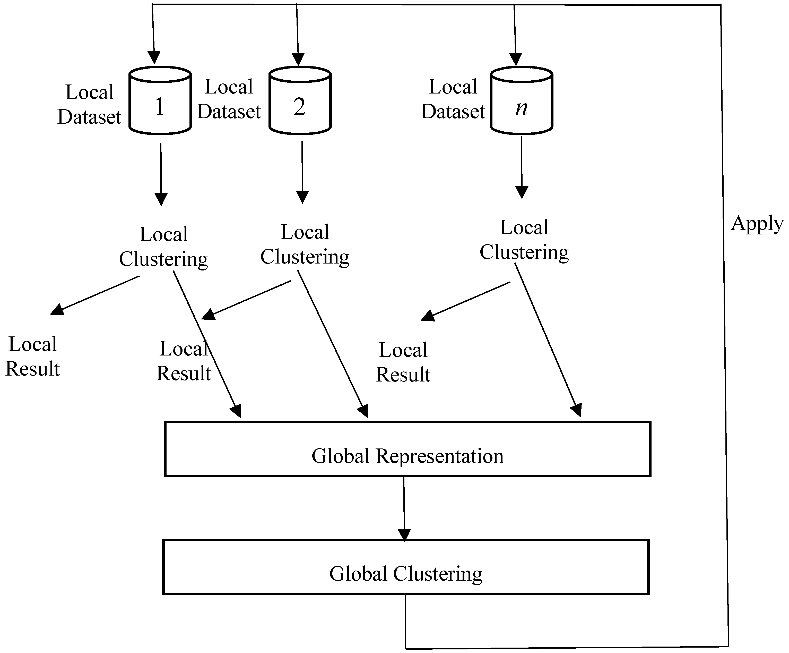
Figure 1. Distributed clustering in homogeneous databases.
Information 10 00144 g001
Figure 2. An example of a heterogeneous dataset.
Information 10 00144 g002
Figure 3. Structure of the deep autoencoder.
Information 10 00144 g003
Figure 4. Deep autoencoder of the local database.
Information 10 00144 g004
Figure 5. Structure of the double deep autoencoder.
Information 10 00144 g005
Figure 6. The performance evaluation of the proposed methods.
Information 10 00144 g006
Table 1. Description of datasets.
DatasetsMnistCovertypeSDDD
Records70,000581,01258,509
Class10711
Replica423
Replica Attributes196/196/196/19610/4416/16/16
Table 2. Parameters for datasets.
DatasetsMnistCovertypeSDDD
Replica network196-500-300-100-10-100-300-500-19610(44)-50-40-30-10-30-40-50-10(44)16-50-30-20-10-20-30-50-16
Server network10-400-200-20-200-400-1010-50-25-10-25-50-1010-40-20-10-20-40-10
Activation functionHyperbolic tangentHyperbolic tangentHyperbolic tangent
Dropout rate0.20.20.2
Mini-batch size100100100
OverfittingSparsity regularizationSparsity regularizationSparsity regularization
Adaptive learningNesterovNesterovNesterov
Loss functionMSEMSEMSE
Stopping criterion600 epochs600 epochs600 epochs
Table 3. Consistent accuracy index (CAI) comparisons between different algorithms.
ClusteringMnistCovertypeSDDD
DDA+K-means0.80600.67440.6837
DDA+SOM0.66410.54270.6832
DDA+Spectral0.80900.75760.7691
Note: DDA is the deep double autoencoder method.
Table 4. Performance of the DDA clustering algorithm.
ACCCentralized DADDA+K-MeansCentralized DADDA+SOMCentralized DADDA+Spectral
Mnist0.76210.73540.73150.70300.79240.7416
Covertype0.56040.55240.44300.43470.64880.6076
SDDD0.66300.65840.66560.65860.75060.7245
Table 5. Classification accuracy of the centralized and proposed methods (Parameters Setting: 70% training set, 30% validation set, 5-fold cross validation).
MnistCovertypeSDDD
Centralized DA+softmax0.99730.67420.7251
Network structure784-500-300-100-1054-50-40-30-1048-50-30-20-10
DDA+softmax0.94080.61230. 6754
Information loss5.66%9.18%6.85%