Article

Methods and Challenges Using Multispectral and Hyperspectral Images for Practical Change Detection Applications

Signal Processing Inc., Rockville, MD 20850, USA
Information 2019, 10(11), 353; https://doi.org/10.3390/info10110353
Submission received: 3 September 2019 / Revised: 7 November 2019 / Accepted: 13 November 2019 / Published: 15 November 2019

Abstract

:
Multispectral (MS) and hyperspectral (HS) images have been successfully and widely used in remote sensing applications such as target detection, change detection, and anomaly detection. In this paper, we aim at reviewing recent change detection papers and raising some challenges and opportunities in the field from a practitioner’s viewpoint using MS and HS images. For example, can we perform change detection using synthetic hyperspectral images? Can we use temporally-fused images to perform change detection? Some of these areas are ongoing and will require more research attention in the coming years. Moreover, in order to understand the context of our paper, some recent and representative algorithms in change detection using MS and HS images are included, and their advantages and disadvantages will be highlighted.

1. Introduction

Multispectral (MS) and hyperspectral (HS) images have more bands than the RGB images. Well-known examples of MS images include Landsat and Worldview images. Landsat has 11 bands [1], and Worldview-3 images have one panchromatic, eight visible and near infrared (VNIR), and eight short-wave infrared (SWIR) bands [2]. The spatial resolution can differ a lot. Landsat has 30 m resolution in most bands, and Worldview-3 has 1.2 m resolution in VNIR bands and 7.5 m in SWIR bands. Examples of HS images include Airborne Visible/Infrared Imaging Spectrometer (AVIRIS) [3] and Adaptive Infrared Imaging Spectroradiometer (AIRIS) [4]. AVIRIS images have 224 bands in the range of 0.4 to 2.5 microns. AIRIS is a longwave infrared (LWIR) sensor with 20 bands for the remote detection of chemical agents such as nerve gas.
MS and HS images have been widely used in fire damage assessment [5], anomaly detection [6,7,8,9,10], chemical agent detection and classification [11], border monitoring [12], target detection [13,14,15], and change detection [16,17]. Due to cost considerations, different imagers need to trade off among spatial, spectral, and temporal resolutions. A high spatial resolution imager normally cannot also have a high spectral resolution, and vice versa. There are over 200 bands in NASA’s future Hyspiri mission, but the spatial resolution is only 60 m [18]. Although Hyspiri [19] intends to provide global coverage, its 60 m resolution is low for many applications such as ship detection in harbors, airplane detection and counting in airports, etc. Some new advances in improving the spatial resolution of MS and HS images have recently been achieved; see [20,21,22] and the references therein. Fusion methods based on pan sharpening have been used to improve the spatial resolution of MS and HS images.
In addition to the above resolution issues in MS and HS images, other research topics exist, such as anomaly detection, change detection, etc. Change detection normally refers to the detection of changes between images collected at two different points in time. For example, counting the number of cars over time in shopping centers will provide business intelligence to shop owners. Another application is related to border monitoring, where illegal trails may be detected by comparing images collected at different times. However, there are some practical issues such as changes due to illumination, misregistration, parallax, etc. Another important issue is computational load, as HS images have hundreds of bands.
It should be mentioned that the goal of this paper is not to provide a comprehensive review of change detection algorithms. Some recent review papers already presented an excellent overview of the algorithms up to 2005 [23], up to 2012 [24,25], and up to 2015 [26]. Instead, we include reviews of about 50 papers published after 2015. Moreover, our goal is to raise some challenges and practical issues in change detection using MS and HS images from a practitioner’s point of view. In the past five years, we have been working on applications such as border monitoring [12,17,27,28], refugee camp growth monitoring [29], Mars exploration using multispectral imagers [30,31,32,33,34], airplane detection using satellite images [29], etc. From those applications, we observed some challenging issues that, in our opinion, have been overlooked by academics, and which are still unresolved. For example, the registration of non-nadir images [35], which are taken from rovers, satellites, or airborne sensors, is still an unsolved problem. Another unsolved problem is about registering two images with different views. Due to non-planar image contents [36], there are still no satisfactory with which methods to align two images. Moreover, we found that the use of synthetic spectral bands can enhance the detection performance in some cases [28,37], but in other cases [29], we did not see much benefit. Other practical issues exist, such as change detection using fused images [38]. All of these observations are drawn from practice, and solving them will be important for many practical applications.
In this paper, we first review some representative change detection methods using MS and HS images in Section 2; more than 50 recent papers after 2015 are included. The advantages and limitations of some representative methods will be mentioned. Some new developments, including multiple sensing modalities, in change detection will be summarized as well. This will lay down the foundation for further discussions. In Section 3, we will mention some challenging directions from practitioners’ viewpoints in this area. For instance, one active research area is to perform change detection using images generated by temporal fusion. Finally, concluding remarks will be given in Section 4.

2. Change Detection Approaches

Here, we will review some representative change detection algorithms for MS/HS images. Since our goal is not a comprehensive review of all past algorithms, we may have missed some of the good papers in this area, which readers are encouraged to peruse [23,24,25,26]. In order to illustrate the performance of different algorithms, we will also include some results for some of them; their advantages and disadvantages will be highlighted.

2.1. Traditional Approaches

Below, we describe some standard approaches in change detection.

2.1.1. Direct Subtraction

Given two images collected at different times, the simplest method is to perform a direct subtraction of the two, with the error indicating the changed areas. Although this method has obvious disadvantages such as errors caused by illumination and shadows, it is very simple and is still being used by many people.
After subtraction, change detection will be carried out by looking for anomalies in the difference image. Some change detection metrics can be used:
Euclidean distance (ED) [39], defined as
f e ( v 1 , v 2 ) = v 1 v 2
where v 1 and v 2 are pixel vectors at times t 1 and t 2 of the same location.
  • Absolute average difference (AAD) [40], defined as
    f a ( v 1 , v 2 ) = | a v g ( v 1 v 2 ) |
  • Vector angle (VA) [41], also known as spectral angle, and defined as
    f v ( v 1 , v 2 ) = arccos ( v 1 T v 2 v 1 × v 2 )
  • Normalized Euclidean distance (NED) [42], defined as
    f n ( v 1 , v 2 ) = ( v 1 v 2 ) / σ
    where σ is the normalized variance of all the pixels in the two images.
It is worth mentioning that change vector analysis (CVA) and its variants belong to this direct subtraction class, and have been widely used in change detection. Details can be found in [26].
Here, we provide a review of a variant of CVA. In a paper by Liu et al. [41], a Sequential Spectral Change Vector Analysis (S2CVA) algorithm was proposed for HS images. It is a semi-automatic approach that can perform multi-level change detection. The first level detects whether there is any change. If there is change, the algorithm goes up one level to detect and discriminate certain change clusters. For each cluster, the algorithm goes up another level to further detect and discriminate smaller clusters within it. The process repeats a number of times.
We will also review another interesting paper on direct subtraction. In [39], Zanetti et al. analyzed the pixel magnitude distribution of the difference of two images collected at two times. The Rayleigh distribution can be used to model the magnitude of unchanged pixels, while the Rician distribution is for modeling the distribution of magnitude of change pixels. Different from conventional approaches, which use approximate Gaussian mixtures to model the distributions, they applied the Expectation-Maximization (EM) algorithm to directly estimate the parameters of the Rayleigh and Rician density models. The proposed algorithm was compared with other methods using synthetic and actual multispectral images, and was demonstrated to yield excellent change detection performance.

2.1.2. Principal Component Analysis (PCA)

Assuming the images at two different times are MS or HS images with multiple bands, the PCA method consists of the following steps [43].
  • For each band, a 2D graph is created in which the X axis is the pixel value from image 1 and the Y axis is the pixel value from the same band in image 2. Each point then will correspond to a location on the images, and the value of each axis will correspond to the pixel value on each image.
  • PCA is performed for the above 2D data and the distance in the second component is considered as the difference between images 1 and 2.
  • The above process is applied to each channel independently. Each change map is thresholded. Change maps from multiple channels are fused by taking the union of all maps.
The above idea was applied to change detection using MS images. Details of the results can be found in [43].

2.1.3. Change Detection Based on Band Ratios

In the literature [43,44,45], there are many variants of band ratios, including the normalized difference of vegetation index (NDVI). People have used these band ratios for land use land cover (LULC) applications.
The NDVI index is used to measure the amount of green vegetation in a given point. The index is calculated in each spatial coordinate of the image as follows:
N D V I W V 2 = N i r 2 R e d N i r 2 + R e d
In the case of the Worldview-2 (WV-2) images, Nir2 is channel 8 and Red is channel 5. Normally, in vegetation change detection between two images at different times, one applies NDVI to each image and identifies the vegetation areas. The changes can be obtained by subtracting the NDVI maps.

2.2. Prediction Based Approach

In Eismann’s book [46], an excellent summary of a prediction-based approach to change detection was presented. The basic idea behind this approach is to match the statistics (up to the second order) of the reference and test images before a subtraction is performed. This will minimize false alarms caused by illuminations. Figure 1 [16] shows a general process of prediction-based change detection, which has two parts:
(1)
Prediction/Transformation. The original reference image (R) and test image (T) are transformed to new spaces as PR and PT. In change detection, the reference image normally refers to an image at an earlier date, and the test image is the image at a later date.
(2)
Change Evaluation. The residual between the transformed image pair is generated. If the interest is only in which pixels have changed, then an anomaly detector is usually applied. If one is more interested in the type of changes, then some additional pixel analyses are needed for the changed areas.

2.2.1. Prediction

Here we mention several representative prediction methods below.
Covariance Equalization (CE) [47]
The core idea in CE is to normalize both the reference and the test images. Mathematically, CE consists of the following steps:
  • Compute mean and covariance of R and T as m R , C R , m T , C T
  • Do eigen-decomposition (or SVD). C R = V R D R V R T , C T = V T D T V T T
    where VR and VT are the orthonormal eigenvectors, and DR and DT are the singular values of R and T.
  • Do the transformation.
    P R ( i ) = V R D R 1 / 2 V R T ( R ( i ) m R ) ,   P T ( i ) = V T D T 1 / 2 V T T ( T ( i ) m T )
Chronochrome (CC) [48]
Compared to CE, CC also computes the cross-covariance between the reference and test images. Details of CC can be summarized below:
  • Calculate means and covariances of R and T as m R , C R , m T , C T
  • Generate cross-covariance between R and T as C T R
  • Perform the transformation.
    P R ( i ) = C T R C R 1 ( R ( i ) m R ) + m T ,   P T = T
According to Eismann [46] and our own experience [16], CC is more accurate if the registration is accurate. On the other hand, CE is more robust to registration errors.
Nonlinear Neural Network (NN)
In CE and CC, second order statistics are matched between the reference and test images. However, this may not be sufficient for some applications. Neural networks (NNs) are well-known for their ability to capture nonlinear behavior between two quantities. We believe that NNs can be used to learn the higher order nonlinear mapping between the reference and the testing image. In papers [16,49], we applied a NN to learn the mapping between R and T. In that work, we used a standard two-layer neural network. Given a MS or HS image with N bands, there will be N inputs and N outputs in the neural network. The neuron number is a design parameter. When the number of neurons is 0, the neural network degenerates to a linear mapping similar to CC or CE. When the number of neurons, K, is non-zero, the NN with a hidden neutron layer is then a nonlinear generalization of the CC or CE methods. Some experimental results are presented in [16] that demonstrate the advantages of using NN over CC and CE. We will also include some results a little later to demonstrate that the NN results are better than CC.
Segmented Linear Prediction (SLP)
The CE, CC, and NN methods all perform well when the statistics are space invariant. In practice, this may not be true. For example, illumination variations due to shadows may be present in different parts of the reference and test images. Such illumination changes may be misinterpreted as real changes, which is not desirable.
In [50], a strategy was proposed to handle the spatially-varying statistics case. The idea is to perform joint spectral clustering of the two images. The pixels at the same locations are stacked together and the joint pixels are clustered. After that, CE and CC are then applied separately to each cluster. Experimental results clearly demonstrated that SLP is much more accurate and more robust to illumination variations.
Local Approaches
An alternative idea to SLP is to perform CE, CC, and NN locally. The local approach can also handle spatial varying statistics, and is very simple to implement. Figure 2 illustrates the local prediction idea. The key steps are as follows:
  • Divide the images into non-overlapped blocks.
  • For each non-overlapped block, pick the prediction windows in the images. The prediction window size is larger than the non-overlapped block.
  • Apply CE, CC, or NN within the prediction window
  • Fill in the block in the predicting image. See Figure 2 [16].
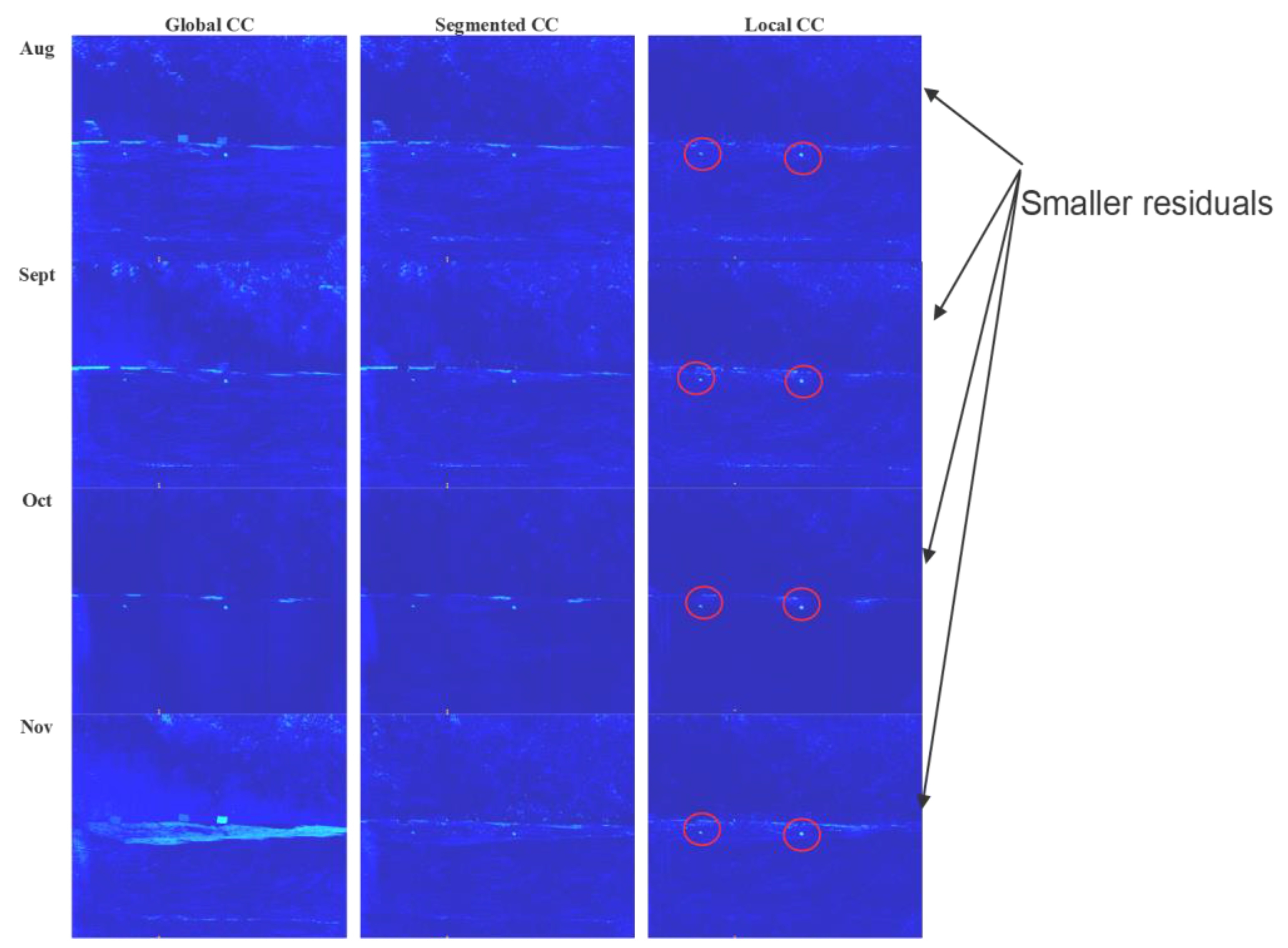
In [16], experiments were carried out to compare the local-based approach and SLP. We include some partial results here. There are four prediction experiments in Figure 3 [16]. Columns one, two, and three show the global CC results, segmented CC results, and local CC results, respectively. One can see that the local CC results gave the lowest residuals, meaning that its prediction is most accurate.

2.2.2. Residual Analysis

After prediction, a difference image will be formed. The ED, AAD, VAD, and NED formulae mentioned in Section 2.1 can be used to perform the change detection. Here, we would like to review several sophisticated methods as well.
RX [51,52]
The Reed-Xiaoli (RX) detector is well-known for the detection of anomalies in MS and HS images. Given a single MS or HS pixel as the test vector in the residual image, the RX-algorithm can be expressed as [52]
RX ( r ) = ( r μ ^ b ) T C ^ b 1 ( r μ ^ b )
where C ^ b and μ ^ b are the covariance matrix and mean of the background pixels, respectively.
KRX [52]
The key idea in Kernel RX (KRX) is to perform RX in the kernel domain where the original pixels are projected to an infinite dimensional space. According to the results in [16,52], kernel RX has better performance than RX. However, the computational load is enormous.
CKRX [16]
Since the computational load of KRX is thousands of time greater than that of RX, a computationally-efficient algorithm known as Cluster Kernel RX (CKRX) was proposed [16]. The key idea was to use cluster centers in the background to compute the detection index. The performance of CKRX is comparable to that of KRX, but with much lower computational cost.
It should be emphasized that many new anomaly detection algorithms have emerged in recent years [53,54]. A separate survey is needed for this area alone.

2.3. Alternative Approaches

Here, we would like to review some alternative developments in change detection.

2.3.1. Change Detection Using Multiple References

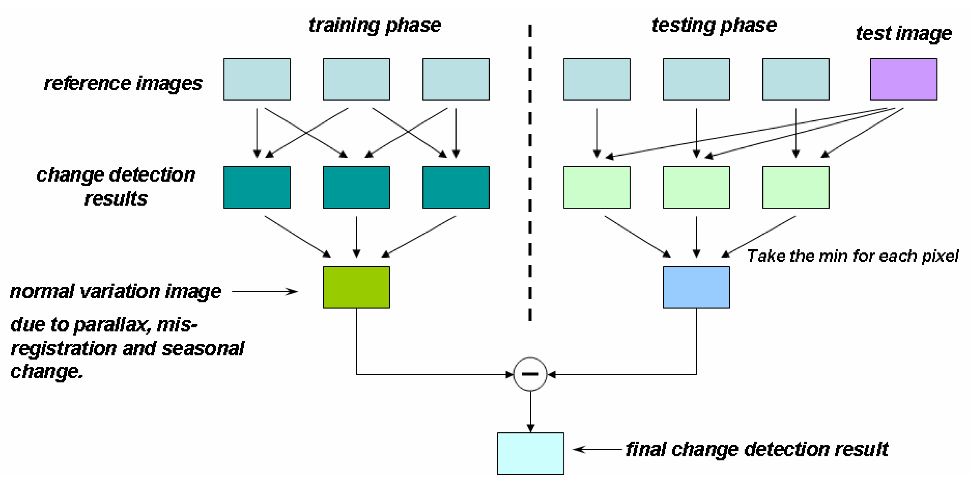
In addition to illumination changes, seasonal changes, and atmospheric effect, it is well known that image registration may not be perfect. In addition, parallax is an important practical issue during data collection. Here, we describe a change detection approach using multiple reference images, if they are available, to alleviate these problems. The Multiple References Change Detection (MRCD) algorithm proposed in [55] is modular, flexible, and nonlinear, as nonlinear operations are involved. Figure 4 [55] shows the signal flow in MRCD. Details of the MRCD are shown below (Algorithm 1).
Algorithm 1. MRCD: (Multiple References Change Detection) [55]
Input: A set of reference images { R i } , a test image T, a single reference change detection function f
Output: Change detection result image O
Algorithm:
  • M i j = f ( R i , R j ) ; f consists of two steps: a) Chronohrome (CC) step; b) anomaly detection
    M = ( M i j ) 1 N ; geometric mean to combine the various Mij into a single image (normal variations)
  • O i = f ( R i , T ) ; use the same change detection function f O = min ( O i ) ; min. operations to minimize false alarms and generate a single change detection image
  • O = O M ; residual image (removes the normal variations in the changes)
    O ( O < 0 ) = 0
    Apply an anomaly detection algorithm such as the RX algorithm [51], KRX [52], or CKRX [16] to the residual image O.
  • Smooth the detection results by using low pass filters to further minimize false alarms

2.3.2. Band Rationing

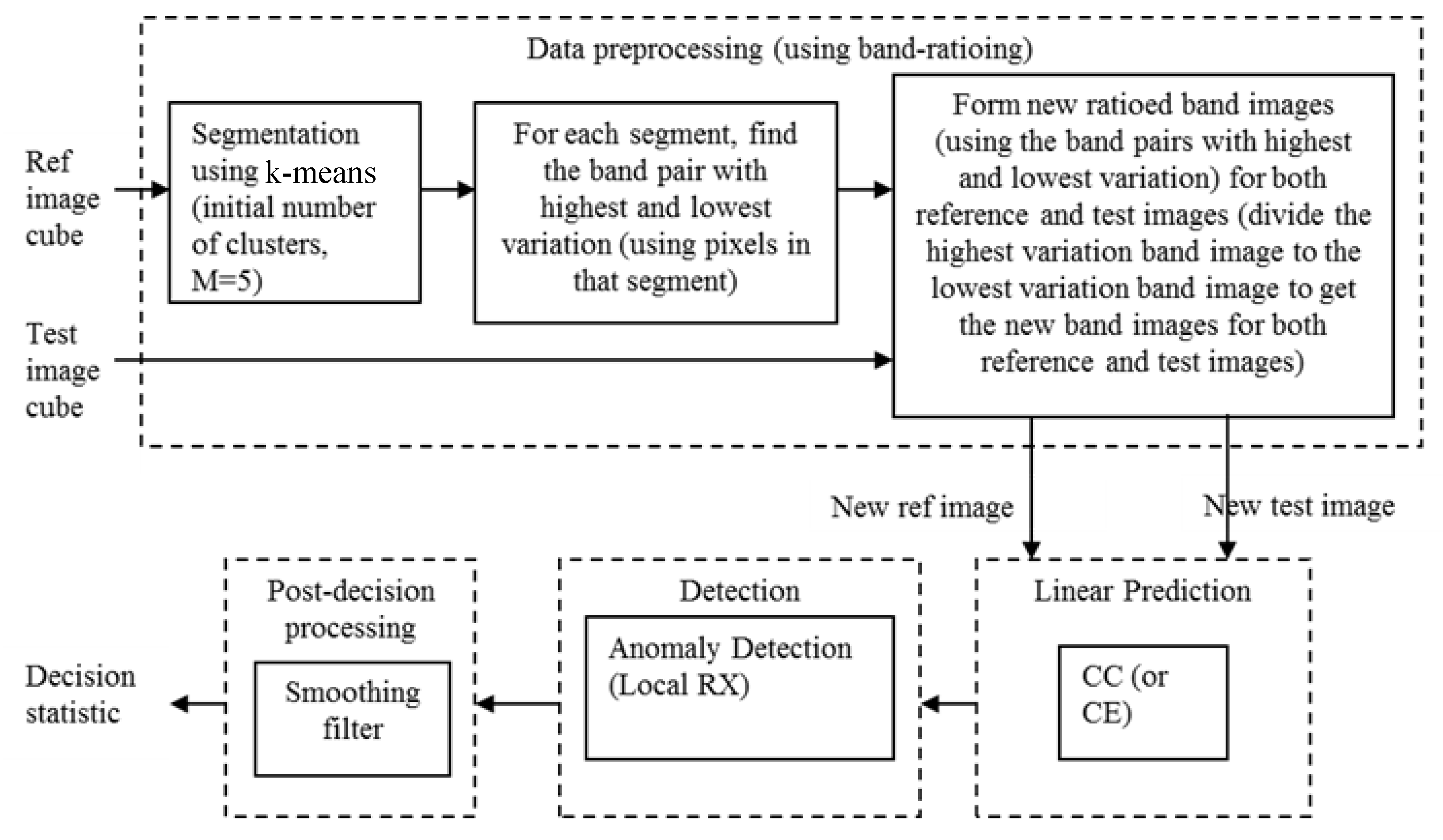
The definition of band-ratioing is simply the ratio of the pixels from two images [44,56]; many variants that are well-known. For example, the normalized difference of vegetation index (NDVI) has been widely used for vegetation detection. A new change detection framework that utilizes new, band-ratioed images was proposed [45]. According to this idea, the reference image cube is first segmented, and for each segment, two bands are determined according to lowest and highest variation in the pixels belonging to the same segment. The new band image is then obtained for both the reference and test image cubes using the same band pair. This has been repeated for all other segments. That is, if there are M segments, there will be at most M new image bands at the end of band-ratioing (for both reference and test image cubes) to be used for change detection. The change detection framework with the band-ratioing idea is introduced in Figure 5 [45]. It can be seen that the architecture is modular and flexible, as we can apply different algorithms in each individual block.
A related paper [57] used a bi-band approach for change detection. There are some similarities between this bi-band approach with that of our work [45]. The bands with maximum and minimum correlations between two images are determined and differenced. Some additional processing will then determine the changed masks. The algorithm contains methods that are easy to implement; yet, the performance in the experiments is quite good using actual data sets.

2.3.3. Deep Learning (Autoencoder)

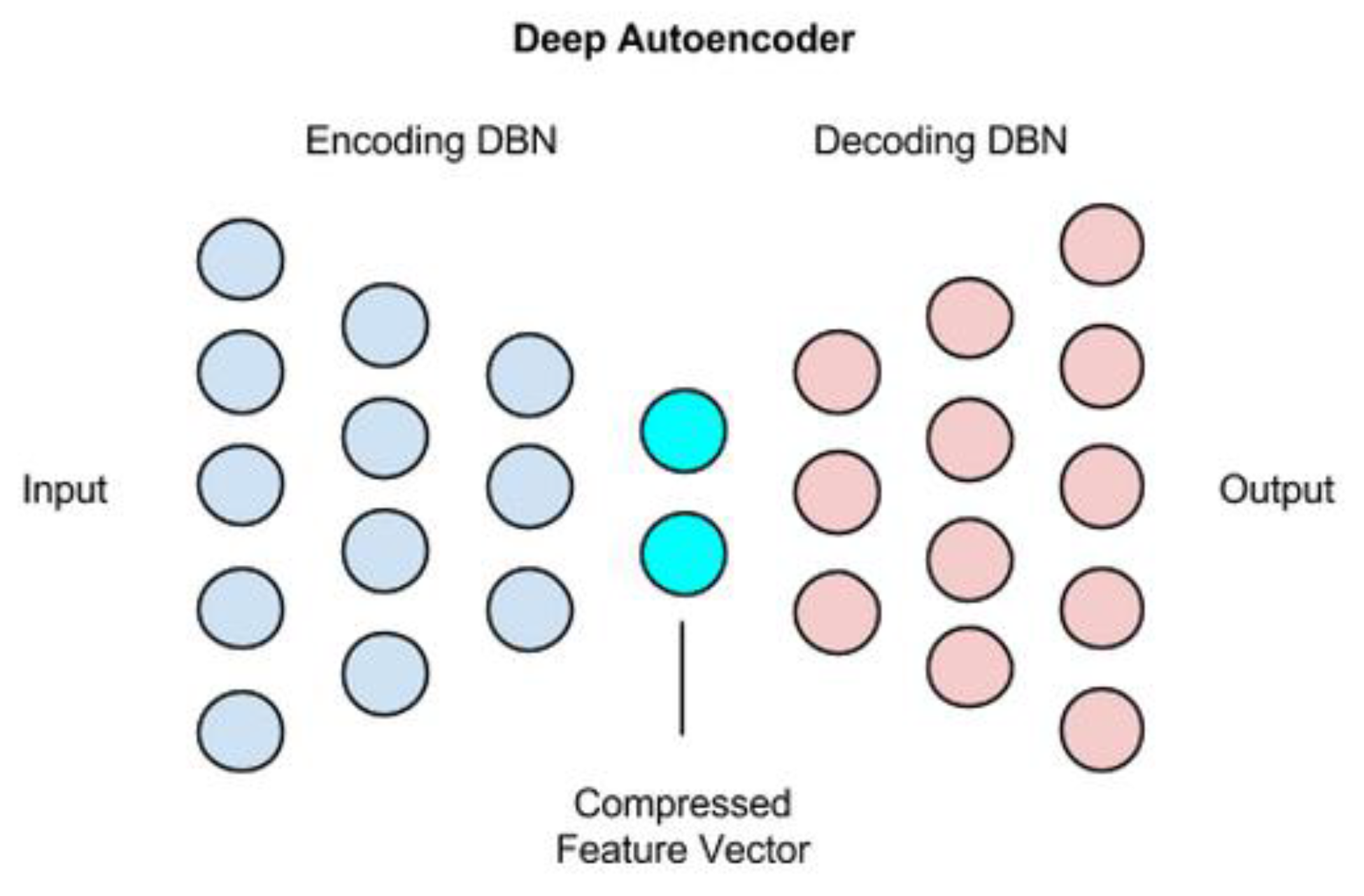
An unsupervised change detection algorithm based on a deep autoencoder was proposed by Xu et al. [58]. The architecture of the auto-encoder is shown in Figure 6 [43]. The idea is to train the autoencoder with patches from image 1 as inputs and patches from image 2 as outputs. The validation data are two sets of the same patches from image 1. Then, to compute the changes, one needs to evaluate all the patches of image 1 in the autoencoder and then subtract each of the decoded patches by their corresponding patch from image 2. Motivated by the work in [58], the following algorithm summarizes the change detection algorithm using an auto-encoder for MS images (Algorithm 2). More details can be found in [43].
Algorithm 2. Change Detection Using Auto-encoder:
Input: Past images {x1, …, xM}; Current image {y}
Output: Change map
Steps:
  For image pairs {xi,y}, i = 1, …, M
  • Collect patches;
  • Patches of xi as inputs to autoencoder and patches of y as outputs. Forward training followed by backward training until steady state has been reached.
  • Subtract y from the predicted y with xi as input
  • Threshold the difference image
  • Repeat for each i
  • Perform an intersection of the of the difference images.
  • Perform a closing to connect the isolated regions and then an erosion operation to remove the isolated regions.

2.3.4. Joint Sparsity Approach

In a paper published in 2018 [59], a new approach was presented to perform change detection using joint sparse representation. The multi-temporal hyperspectral images are first stacked together. Then, a dual window around the test pixel is used to select local neighborhood pixels. If the test pixel is changed, its reconstruction coefficients will be different. Interested readers can refer to [59] for details.

2.4. Other Approaches

In [26], alternative approaches are mentioned. Statistical methods such as [39,60] have been used in CVA analyses. Experimental results showed that the change detection results can almost approach optimal performance using some satellite images. Morphological methods such as the one in [61] are also mentioned in [26]. Finally, in the classification-based change detection methods mentioned in [26], pixel classification algorithms are applied to two images separately, and changes are detected via some post-classification analysis.
We would like to point out some papers in change detection using heterogeneous images. For example, one may want to detect changes between an earlier SAR image and a later optical image, and vice versa, for the same area. Some representative papers [62,63,64,65,66,67] have been published in recent years. This research is very challenging, and more research is needed. We have also started to work in this area.

2.5. Survey of Approaches After 2015

Here, we summarize a survey of close to 50 change detection papers after published after 2015. We divide them into three groups: supervised, unsupervised, and applications. At the end of each subsection, a table summarizing the papers will be provided.

2.5.1. Supervised

The paper in [67] presents a supervised change detection approach for urban areas that has several key characteristics: the first is a feature selection process using two thresholds; the second is the utilization of both spatial and spectral features for change detection; the third is the use of multiple classifiers (extreme learning machine (ELM), multinomial logistic regression (MLR), and K-nearest neighbor (KNN) classifiers). High resolution satellite images (ZY-3) were used for performance evaluation. The proposed method yields better results than existing methods.
A paper by Wang et al. [68] is similar in spirit to [67]. It is an object-based approach that requires the segmentation of objects. Spectral, spatial, and textual features are extracted and then used to generate difference maps. Finally, several supervised classifiers (k-nearest neighbor, SVM, extreme learning machine, and random forest) are used for change detection. Two high-resolution satellite image sets were used in the evaluation.
The advantage of [67,68] is that the proposed approaches are easy to implement. The disadvantage is that it requires a lot of training data, which may be hard to obtain.
It is well-known that VHR images have low class separability. A supervised change detection approach is proposed in [69] based on relationship learning. It begins with enriching the training samples based on their neighborhood relationship and label coherence; this relationship is then learned simultaneously with the classifier. Experiments using actual VHR satellite images demonstrated the performance. The key advantage is that this approach can handle the low class separability issue. However, one potential limitation is that the learned relationship is image dependent, and may be difficult for use with other types of images comprising different contents.
In a paper by Wu et al. [70], the authors propose a scene change detection method via kernel slow feature analysis (KSFA) and post-classification fusion. Experiments with high-resolution remote sensing image scene data sets demonstrated high levels of accuracy in scene change detection. However, it was observed that the Bayesian fusion technique is sensitive to the quality of the estimated change probability.
A paper by Zhang et al. [71] presents a semi-automatic approach that incorporates spatial and spectral features for change detection. Spatial features are used via multiscale feature extraction. The semi-automatic learning part refers to the process of improving the contribution of training samples to the trained model. Applications to two urban data sets (Landsat 7) demonstrated the performance of the proposed approach as compared to some conventional methods such as CVA. However, one obvious drawback of this approach is that it requires human intervention in selecting the training samples, which may be impractical for large-scale applications.
Feature selection is a critical step in image segmentation, which consequently plays an important role in object-based change detection. The paper by Chen et al. [72] applies a genetic particle swarm optimization algorithm to select the best features for segmentation. Experimental results using real data showed that the overall accuracy in change detection exceeded 80%. Although the optimization is insensitive to the initial parameter settings, the performance is sensitive to the number of features and the size of the swarm.
A paper by Hou et al. [73] focuses on building detection. The approach combines pixel- and object-based methods. In the pixel-based method, extended morphological attribute profiles (EMAP) are used in the classification step. In the object-based method, a semi-supervised classification approach based on a random forest is applied. The use of EMAP is similar in spirit to the method described in [37]. There are two limitations according to the authors of [73]: one is the selection of discriminative features, and the other is the selection of the algorithm parameters.
In a paper by Yu et al. [74], the authors proposed a supervised change detection framework. First, unsupervised k-means clustering is used to select representative objects. Users are required to determine which of the samples are “change” or “no change”. Second, active learning via a Gaussian process is used to detect changes. The learning stops when there are no changes in the detection results. Finally, contextual constraints such as color and textures are added via the MRF model. A graph cut is used to generate the final change map. Two data sets of Worldview-2 images were used for performance evaluation. One key limitation of this approach is that users need to be constantly involved in the process, which may be impractical for large area change detections.
One problem in object-based change detection is the scaling issue, which refers to the size of the area of interest. A paper by Feng et al. [75] solves this issue using an object-based approach to urban area change detection (CD). The approach contains a rotation forest (RoF) and coarse-to-fine uncertainty analyses of multi-temporal images. Two HR data sets from Gaofeng imagery were used as a demonstration. It is not clear whether the method can be generalized to other satellite images such as Worldview images, which are collected from non-nadir views with different slant angles. As a result, the building shapes may be very different from image to image.
It is well-known that some pixel-based change detection methods do not exploit spatial information, and that object-based methods have segmentation errors. The paper by Tan et al. [76] focused on change detection using multiple classifiers. Various spatial features such as textures and gradient information are extracted first. The features are used for object classification. Different classifiers such as SVM, CVA, and KNN are then fused using the Dempster Shafer algorithm for change classification. Although the idea is straightforward, the authors have paid attention to the details. Consequently, the experimental results are quite good. One potential improvement is perhaps to incorporate some newer algorithms such as sparsity and deep-learning-based methods into the fusion paradigm.
The following are some representative and recent papers [77,78,79,80,81] based on sparsity optimization.
Chen and Wang [77] proposed a Spectrally-Spatially (SS) Regularized Low-Rank and Sparse Decomposition (LRSD) model. The SCV is decomposed into a locally-smoothed, low-rank matrix, a sparse matrix, and an error matrix for noise. Both synthetic and real-world data sets were used in the experiments.
A paper by Erturk et al. [78] proposed dictionary pruning for hyperspectral change detection using sparse unmixing. Both synthetic and real datasets were used to validate the proposed approach.
In the following few paragraphs, we will summarize some deep-learning-based methods for change detection.
A paper by Wu et al. [79] addresses a practical problem in change detection when only low-resolution images are frequently available. The authors proposed an algorithm that first generates fractional maps from the low-resolution images. The HR image is used to train a neural network for sub-pixel classification. Once trained, the NN can be used to classify the fractional maps in the first step at each time. Finally, the changes can be detected using the sub-pixel classification maps. Experiments using both actual and synthetic data demonstrated the performance.
A Spectral-Spatial Joint Learning Network (SSJLN) was proposed in [80]. The key advantage is that both spectral and spatial information is taken into account. Although the performance is good, the approach requires training data, which may be difficult to obtain in practice.
Wang et al. [81] proposed an algorithm that first applies linear and nonlinear unmixing methods to extract the abundance maps from the input images, which are then used to a create mixed affinity matrix. The affinity matrix is then fed into a CNN network for change detection. Experiments verified the performance of the approach. One key advantage is that only the input images are needed for CNN training.
It should be noted that in all of the aforementioned sparsity-based approaches, the construction of the dictionary may be a concern for practical applications. This is because the performance relies heavily on the choice of the atoms in the dictionary. Moreover, the process requires human intervention and is tedious, and also dependent on experience.
The following few papers [82,83,84] are related to deep learning.
A paper by Lyu et al. [82] was the first on the application of deep-learning-based recurrent neural networks for change detection. The proposed method learns a change rule, and the learned rule can be transferred to new target images. Experiments using Landsat and Hyperion images validated the proposed algorithm.
Song et al. [83] present a change detection framework for hyperspectral images using recurrent convolutional neural networks. The first step is the use of PCA to help select training samples. The second step is the use of recurrent CNN for training and testing. Experiments using Hyperion images showed that the proposed approach can be useful for both binary and multi-class change detection.
In [84], Ma et al. present a heterogeneous change detection algorithm between a synthetic aperture radar (SAR) image and an optical image. The first step is the mapping, which requires the use of some unchanged areas in both images. The pixels are then transformed based on their distance from the changed areas. After the transformation, the two images are then fed into a capsule network for change detection. The capsule network was introduced by Hinton in 2017, and has gained attention since then. The proposed framework was evaluated using both homogeneous and heterogeneous data sets.
Common to all the deep learning approaches mentioned above is the fact that vast amounts of training data are required. It is well known that if the training data are not sufficient in deep learning, then generalization to new images may suffer tremendously.
We follow the tabular format in [26] and create a table summarizing the above papers in Table 1. We categorize the methods into four groups, which are by no means unique. Different authors may have different arrangements. The table contents are complementary to our reviews, in that some notes and data types are included.

2.5.2. Unsupervised

A paper by Liu et al. [85] presents a hierarchical CD approach that can detect multiple levels of changes based on pixel spectral behaviors. Synthetic and real data were used for algorithm verification. One issue with the hierarchical approach appears to be ad hoc, and there are no guidelines on how many levels are sufficient for certain images.
In a paper by Zhuang et al. [86], the authors combined change vector analyses (CVA) and a spectral angle mapper (SAM) for unsupervised change detection. Two strategies were presented which are easy to implement. Synthetic and actual data were used in the performance evaluation. The method is analogous to weighted fusion, and one potential drawback is that the weighting needs to be determined through trial and error.
A paper by Liu et al. [87] presents a novel multi-temporal spectral unmixing (MSU) approach to change detection in HS images. The first step is to perform multi-temporal endmember extraction. The second step is a change analysis to distinguish change and no-change based on the endmembers. Finally, abundance analysis is applied to each pixel for multiple class change detection. Real data were used in the performance evaluation. One potential limitation is that the endmembers need to be known in advance. Moreover, there is no analysis on what happens if the available endmembers are fewer than the actual endmembers.
A new similarity space was proposed in [88] to increase the separation between change and no-change classes. Comparative studies were carried with some standard change detection methods such as image differencing, SAM, and rationing. It would have been good if the authors had included some newer methods in their experiments.
The title of the paper by Shao et al. [89] is a little confusing, as it is unclear whether the approach is unsupervised or semi-supervised. The first key idea is to combine three information types (intensity, labels, and spatial context) in the difference images. The second key idea is a segmentation algorithm for change detection using the above information. Six experiments using various Landsat and SAR images demonstrated the performance of the proposed algorithm. Since the method relies on the direct difference of two images, image registration errors may throw off its accuracy. The authors did not address the robustness issues of their algorithm. Moreover, the comparative study did not include some commonly-used algorithms such as CC or CE.
A paper by Ma et al. [90] focuses on object-based change detection. A comparative study was carried out for four methods in the literature. The objective was to evaluate the four algorithms using different segmentation strategies on two WorldView-2 images. Since segmentation performance depends on threshold, the authors did not provide a threshold selection strategy, and more research appears to be needed in that direction.
Although the title of the paper by Liu et al. [91] mentions change detection using random walks, there are actually some other techniques (PCA and GMM) involved in the process. It is also not clear whether the overall approach is unsupervised, because GMM requires some training data. In any event, the proposed framework appears to work well for several diverse imagers (Landsat, ASTER, and Quickbird).
The idea presented in a paper by Wang et al. [92] is interesting. The key innovation is to generate four cross pansharpened images for a given pair of MS images with pan band. The change detection algorithm used is the iteratively reweighted multivariate alteration detection (IR-MAD) method. According to [92], the proposed method yielded good change detection results in water and vegetation areas. One issue with this paper is that only one method (IR-MAD) was used, while other state-of-the-art methods, and perhaps better and newer algorithms, were not.
A paper by Liu et al. [93] presents both unsupervised and supervised band selection-based, dimensional reduction techniques. The reduced dimension data are then used for change detection. The authors found that using reduced dimension bands allowed their approach to outperform some other change detection methods that use the full bands. Although reduced dimension data can speed up the computations with minimal or no loss of performance, the paper did not provide guidelines on about how many bands are needed for a given data set. Users need to experiment with the number of bands, and this may be a practical issue in applications.
A paper by Lu et al. [94] focuses on the post-processing step in the change detection process, which tries to enhance the change detection maps. In particular, the authors proposed an object-based expectation maximization (OBEM) method that considers multi-scale segmentation and expectation maximum algorithms. Experiments using three images (aerial and satellite) demonstrated the performance of the proposed approach. The authors claim that their approach is applicable to VHR images. However, two out of four images are actually of low resolution. Moreover, focusing on post-processing may not be the best approach in practice; an end-to-end approach encompassing preprocessing, change detection, and post-processing may be needed.
In [95], the authors proposed a change detection approach in VHR optical images. The key idea is to transform images via transformation to some common features. For example, tasseled caps transform is used in this paper for image transformation. Experiments using different multispectral sensor data were used in the evaluation of the algorithm. At the end of the paper, the authors highlighted a few future directions to address some limitations in the paper, including associating clusters with certain types of changes, feature selection to further separate different changes, etc.
The idea proposed in [96] is quite simple, and the goal is to address the issue of when the spectral shapes between changed and unchanged pixels are close. Spectral shapes, the gradient of spectral shape, and Euclidean difference between spectral shapes are used separately for change detection. A weighted fusion is then used to combine the change detection maps. The last step needs human intervention, which can be considered as a limitation of the method. Experiments showed that the results were good.
A paper by Park et al. [97] presents an interesting and unsupervised approach to change detection. The key idea is the use of cross-sharpened images, as used in another paper [92], to reduce false alarms due to relief displacement and seasonal changes. A cross-sharpened image is generated when the pan band is collected at a different time from that of the MS bands. A sequential spectral change vector analysis (S2CVA) is then applied to the various combinations of difference images. KOMPSAT-2 satellite images were used for the performance evaluation. One critical comment is that this paper only focused on S2CVA, and did not compare its approach with other state-of-the-art methods. Hence, it is hard to judge whether the proposed method is indeed better than others.
A paper by Lei et al. [98] presents an unsupervised fuzzy clustering approach for landslide detection. The first step uses fuzzy c-means to generate landslide candidates. The second step utilizes differences in image structure instead of pixel difference for landslide localization. High resolution aerial images (3-band) collected in three locations in Hong Kong were used for algorithm validation. The paper only compares the novel approach with three methods. It would have been good to see a more thorough comparative study with some modern change detection methods which are described in the literature.
A paper by Li et al. [99] is very interesting, in the sense that even though it uses deep learning for change detection, the approach is actually an unsupervised one. One key innovation is the utilization of the change detection maps of existing unsupervised change detection methods to train the deep CNN. Hyperion images were used in the experiments. This is a promising approach, as it allows deep learning to succeed without using supervised training data.
Table 2 summarizes the papers in this subsection. We tried to group some papers that use similar methods. However, the methods are more diverse than those in Table 1.

2.5.3. Applications

Change detection algorithms have been used in many applications such as arid environment monitoring [100], submerged biomasses in shallow coastal water [101], phragmites australis distribution [102], etc. We will mention some other applications in the following paragraphs.
A paper by Ballanti et al. [103] used an object-oriented approach that performs hierarchical classification using commercial software (eCognition Developer) to identify changes within the watershed and wetland ecosystems. Data for the Nisqually River Delta between 1957 and 2015 were used for case studies. The changes are determined based on the classification results. During that time span, there should be some Landsat images available for some years. It is a surprise that the authors did not use Landsat images in their study.
Lv et al. [104] present some practical methods to determine changes in the change detection process: the first deals with noise reduction; the second helps the threshold selection process; and the third focuses on region growing. The authors claimed that these tools can make change detection almost automatic, which is very important in practice. Four date sets were used in the evaluation. After examining the algorithm closely, it was noticed that some decision thresholds are still needed in the region growth algorithm, which means that the algorithm is not “almost automatic”.
The paper by Lv et al. [105] talks about using textual information around a pixel as a basis for comparing the changes in two images. The algorithm is easy to follow and the results are quite good when compared to several existing methods using three data sets. However, the experiments only compared the described approach with other textual based methods. It is unclear how good this method is compared to non-textual methods such as CVA or CC. Although the paper talks about change detection between homogeneous images, the same idea may be applicable to heterogeneous images.
In [106], the authors applied Dempster Shafer (DS) fusion to combine several change detectors for urban change detection. The idea is simple, but effective, as demonstrated in the two experiments described in the paper. However, as admitted by the authors, one key limitation of this approach is that there are many parameters that need to customized, making it very demanding from the users’ point of view.
In a paper by Liu et al. [107], the authors explored the use shape features such as lines in buildings, and an object-based approach to enhance building change detection. It was demonstrated that the building change detection performance had been improved using actual satellite images. One limitation of the line features is that some non-building structures such as roads, pavements, cars, etc. may also have strong line features, thereby degrading the overall change detection performance.
A paper by Zhou et al. [108] focuses on coral reef change detection. The key contribution is the comparison of object-and pixel-based algorithms. The object-based approach involves image segmentation, random forest models, and image fusion. It was observed that, using Quickbird and Worlview-2 images, the authors were able to demonstrate that the object-based approach could yield 20% better accuracy than the pixel-based approach. The above observation may be an over-statement, as there are pixel-based algorithms [5,12,37] that utilize both spectral and neighboring spatial information to perform joint change detection.
In [109], the authors present an interesting approach to change detection that incorporates both 2D and 3D information. The 3D information refers to terrain information. Four test cases using aerial images were used for a performance demonstration. One potential limitation is that the approach assumes accurate coregistration of 2D and 3D images. As will be mentioned in Section 3, registration is challenging, even for images of the same type.
The recognition of some built-up areas is seriously affected by seasonal changes. In [110], the authors discuss the use of various spectral indices, spectral classification, and morphological processing to recognize built-up areas in Yakutsk. In addition, socio-economic modeling was also performed. Sentinel and Spot 6 images were used in the study. Although the various methods are standard and not novel, the authors have done a good job at customizing the algorithms, yielding reasonable results. The authors mentioned that, in their approach, the separation of bare soil from built-up areas is a key difficulty that needs further investigation. We suggest that the soil detection problem can be addressed using the methods described in [27,28,37].
Change detection for deforestation is affected by seasonal variations in weather. In [111], the authors explicitly take SWIR-2 in Landsat to improve the change detection performance. In particular, object-based image analysis (OBIA) combined with a Random Forest (RF) is proposed to discriminate deforestation from seasonal changes. Experiments using actual Landsat images demonstrated that 88% accuracy was achieved for the studied areas. As mentioned in the paper, there are some limitations of the approach, including sampling considerations, timing of changes, application to large datasets, and deforestation occurrence. More research is needed for deforestation monitoring.
In a paper by Gong et al. [112], the authors first applied a deep convolutional network to obtain building proposals. After that, corner and edge information were integrated for feature detection and roof matching. Finally, a co-refinement strategy based on a conditional random field (CRF) was used to classify buildings as “newly built,” “demolished”, or “changed”. Experimental results using aerial images showed more than 85% accuracy for building change detection. One limitation is that the proposed approach is sensitive to segmentation accuracy. Another limitation is that the patch matching performance may be poor when the roofs do not have distinct features.
The above papers are summarized in Table 3. As shown, there are many diverse applications in the table.

3. Challenges in Change Detection from Practitioners’ Viewpoints

Despite intensive research in change detection using MS and HS images over the past two decades, there are still quite a few challenging and important problems. Here, we mention some of them from practitioners’ points of view.

3.1. Need to Enhance Registration Performance

Since the performance of change detection algorithms depends heavily on the accuracy of registration, it is critical to have registration algorithms that can reach sub-pixel accuracies. For images collected at nadir, feature-based algorithms based on SIFT or SURF perform quite well. However, for images collected off-nadir, feature-based algorithms can cause big errors. For example, Worldview images are normally collected off-nadir, as one can see the sides of buildings. More research in robust and accurate registration algorithms is still needed for the handling off-nadir images.
To handle registration errors, one possible remedy is to resort to robust prediction algorithms. As mentioned earlier, Eismann [46] did a comparative study. CE [47] is more robust than CC [48] when there are large registration errors. The use of nonlinear NN [16] was also demonstrated to perform better prediction than CE and CC.
The paper by Marchesi et al. [113] presents an adaptive technique that mitigates the registration noise on very high resolution (VHR) images. The first step is to identify registration noise; the second is a context-sensitive decision strategy to create the final change-detection map. Experiments using actual images demonstrated the performance.
Although there are papers such as CE [47] and the method in [113] that can perform robust change detection in the presence of registration errors, more research on other robust algorithms could be interesting.
A related paper [114] also discussed an approach that is robust to misregistration errors that are less than one pixel. The key ideas are summarized in Figure 1 and Figure 2 of [114]. Each 3×3 block is divided into four quadrants, and each quadrant has nine parameters that can be optimized to compensate for misregistration errors. Several data sets were used to validate the proposed algorithms. One notable limitation of the approach is that roof matching can be erratic due to lack of textual features.

3.2. Need to Improve Computational Efficiency

Because of hundreds of bands, more computations are needed for hyperspectral images compared to MS images. Researchers have experimented with numerous ways to reduce computations for HS images. A well-known technique is to apply PCA to compress hundreds of bands into only ten or fewer bands. In [15,115], the researchers developed target detection algorithms directly in the radiance domain instead of the reflectance domain. As a result, only a small number of target signatures need to be converted from reflectance to radiance, and hence, a great reduction of computations has been achieved. Similarly, there are fast anomaly detectors based on random down sampling of background pixels [116], cluster centers of background pixels [16], progressive line scanning [53], and recursive implementation [117].
For local change detection, parallel processing using multi-core CPUs and GPUs may be another future direction.

3.3. Possibility of Change Detection Using Enhanced MS and HS Images

In some recent studies [12,18], it was observed that high spatial resolution images can enhance target detection performance. Similarly, we believe that the change detection performance may also be improved if high resolution images are available.

3.3.1. Enhancing the Spatial Resolution of MS Images

A well-known approach to enhancing the MS image resolution is via pansharpening, which uses the HR pan band to enhance LR MS images. However, in some cases where the LR MS bands consist of different spectral ranges, some new techniques may yield even better performance in terms of spatial resolution.
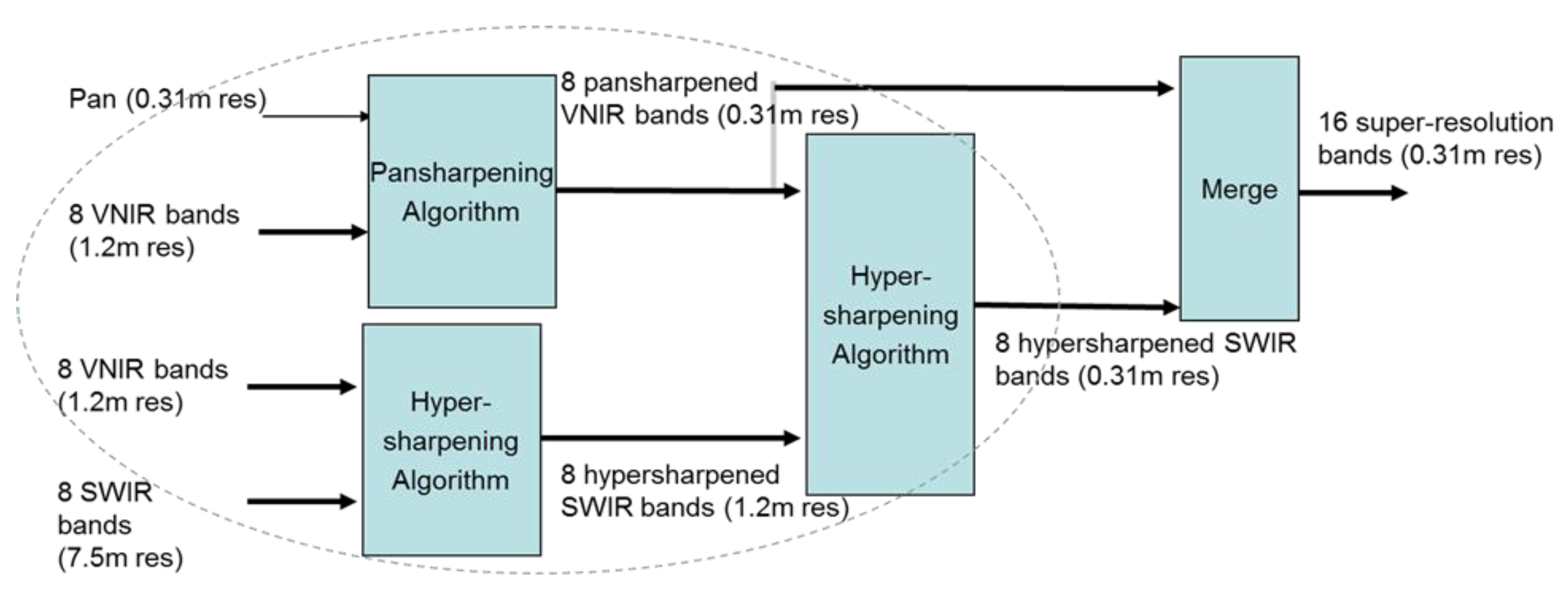
Let us consider the Worldview-3 images, which have one HR pan (0.5 m), eight VNIR (2 m) bands, and eight LR SWIR bands (7.5 m). Conventional algorithms apply pansharpening to the VNIR and SWIR bands separately. Recently [2,118], three new additional approaches were proposed to pansharpen the SWIR bands. Below, we show a block diagram of the best performing approach (Approach 4). Figure 7 [119] shows Approach 4, which begins with a parallel pansharpening step, followed by a sequential step. The experimental results in [2] showed that Approach 4 yielded the best performance.

3.3.2. Spatial Resolution Enhancement for HS Images

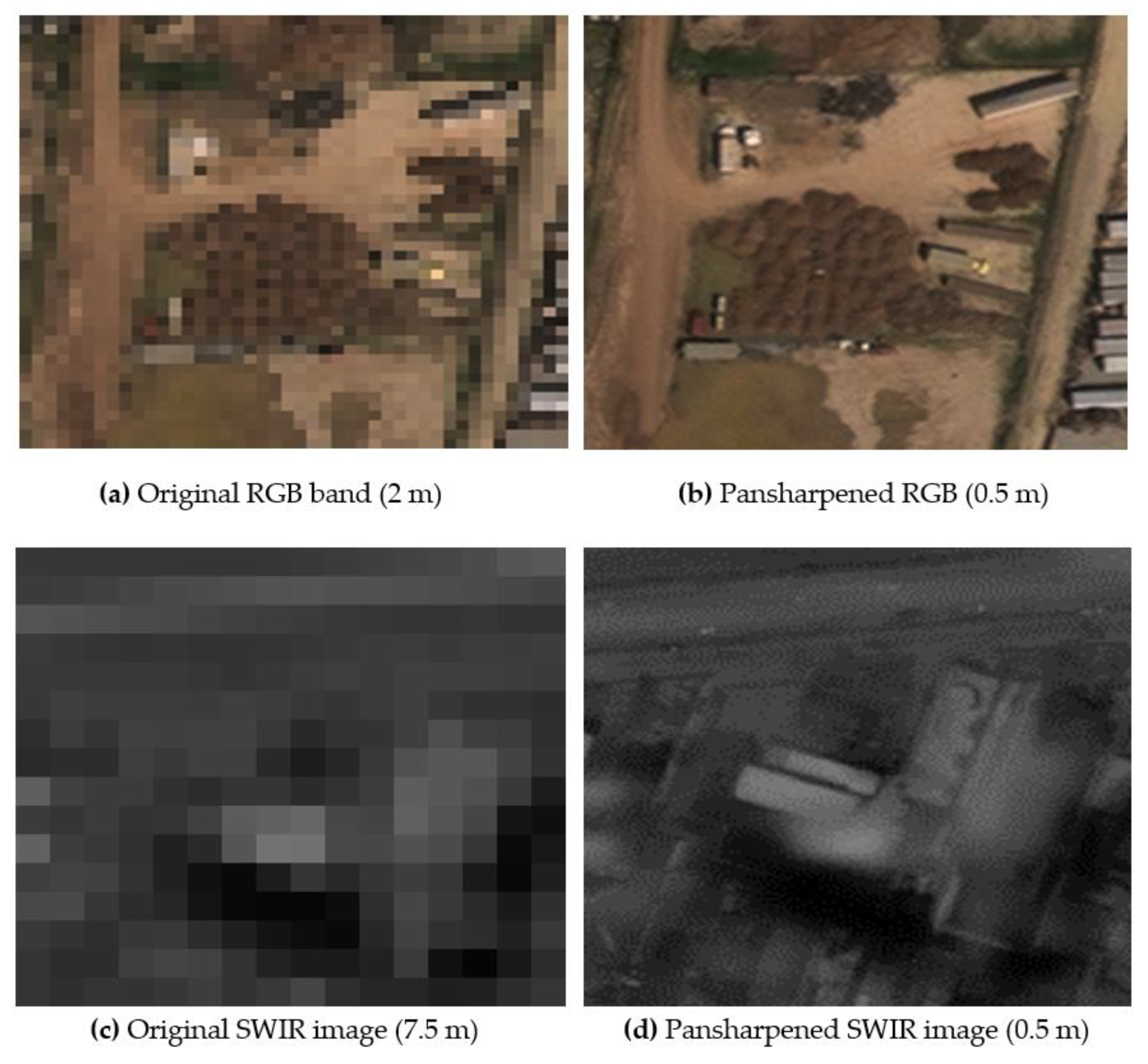
In order to illustrate our point that high resolution HS images can improve the target detection performance, we would like to include some results on soil detection for illegal tunnel detection. The objective is to use satellite images to detect excavated soil from illegal tunnel digging. Figure 8 [12] shows the enhanced pansharpened images in the multispectral and shortwave infrared (SWIR) ranges. As can be seen from Table 1 in [12] for a particular test date, the soil detection performance using joint sparse representation (JSR) [12], kernel JSR [12], matched subspace detector (MSD) [119], kernel MSD (KerMSD) [120], Support Vector Machine (SVM) [121], and pixel-wise sparse representation (SR) [122] methods have seen strong improvement after pansharpening. Details can be found in [12].
We expect that the change detection performance will be improved if spatial resolution is enhanced. However, there are some practical issues that need to be researched.
Single Image Super-resolution Methods
Here, the spatial resolution of each band in the HS image is improved without using additional images such as the pan band or some other color, or MS images from other imagers. Bicubic interpolation is the simplest and most widely used method which does not utilize the point spread function (PSF) [123]. One recent algorithm [124] utilizes PSF, if available, to improve the resolution of a single image by deblurring. The algorithm in [125] is an edge-interpolation-based method. Deep learning [126,127] -based algorithms have been applied to single image super-resolution. Strictly speaking, deep-learning-based algorithms should be called single image super-resolution, as a lot of training images are required. Dictionary-based approaches [128,129] are also explored. It should be noted that it is very difficult to obtain a lot of training images in remote sensing, making the deep learning and dictionary approaches not very practical. It is our hope that the remote sensing community can work together to build a large image database so that deep learning and dictionary-based algorithms can be compared and evaluated.
Difficulty in Carrying out Pansharpening
Pansharpening algorithms [124,125,126,127,128,129,130,131,132,133,134,135,136,137,138,139,140,141,142,143,144,145,146,147] have been shown to improve the spatial resolution of HS images. However, one prerequisite is the availability of high-resolution pan or color or MS images. When only LR HS images are available, it is very challenging to improve the spatial resolution, except that of using single super-resolution methods. We list some of the challenges in pansharpening below:
  • Lack of data
    In a recent article [38], some recommendations are made on how to collect HS images. The idea is to collect more HR images so that deep-learning-based algorithms can have more training data. For details, see [38].
  • Pansharpening performance assessment
    In practical applications, there is no ground truth images available to assess the pansharpening performance. A full resolution approach [22] is needed. However, existing full resolution assessment methods such as Quality with No Reference (QNR) are still inconsistent, because the best performing method based on QNR may not be the best method based on the peak-signal-to-noise ratio (PSNR). It may require the whole community to address this critical issue.

3.4. Possibility of Change Detection Using Synthetic HS Images

In some applications, only LR MS images are available. Will we be able to synthesize some hyperspectral images using those images? The authors of [146] worked on spectral band synthesis. Since then, there have been some new algorithms such as the Extended Morphological Attribute Profiles (EMAP) algorithm [147].
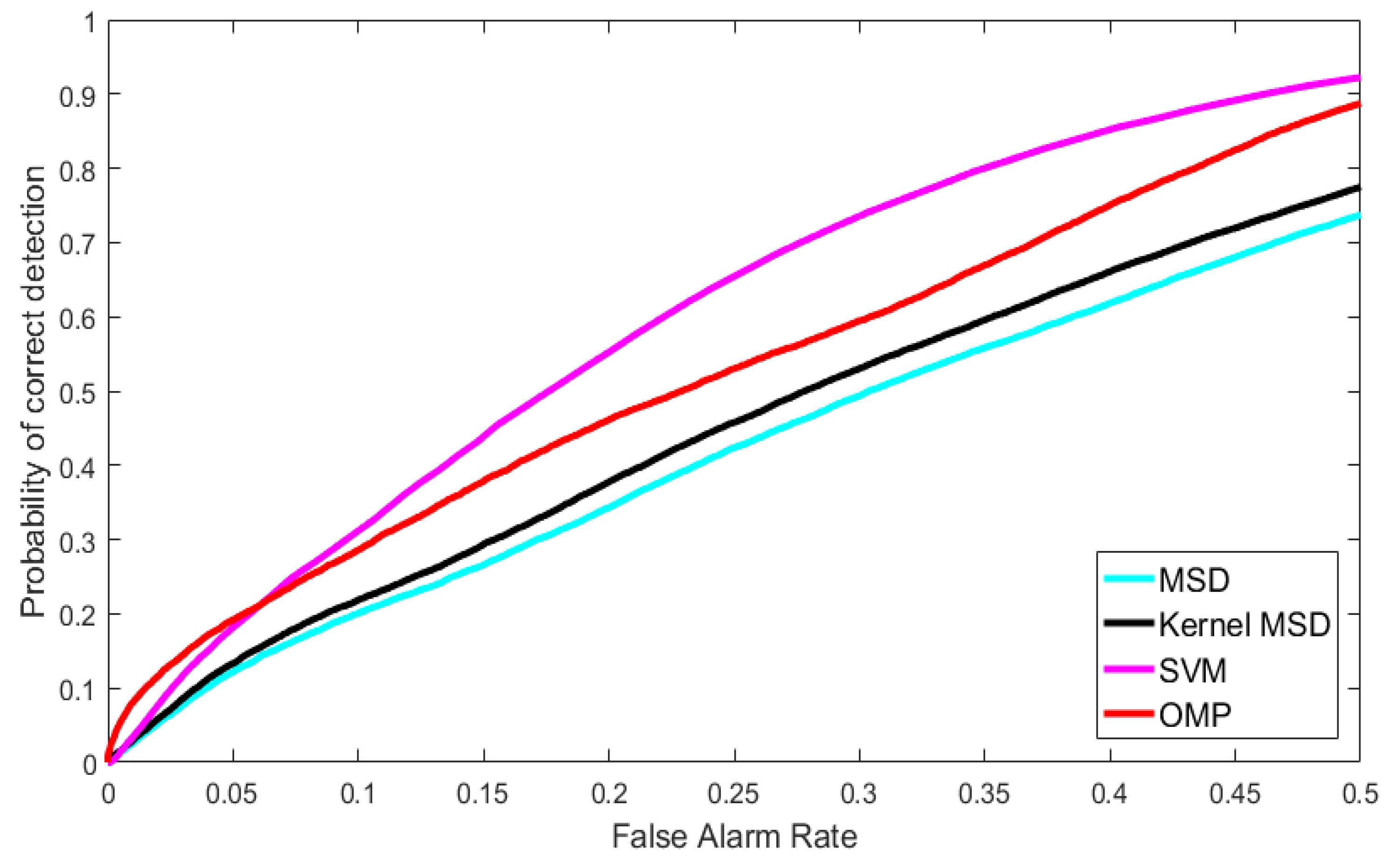
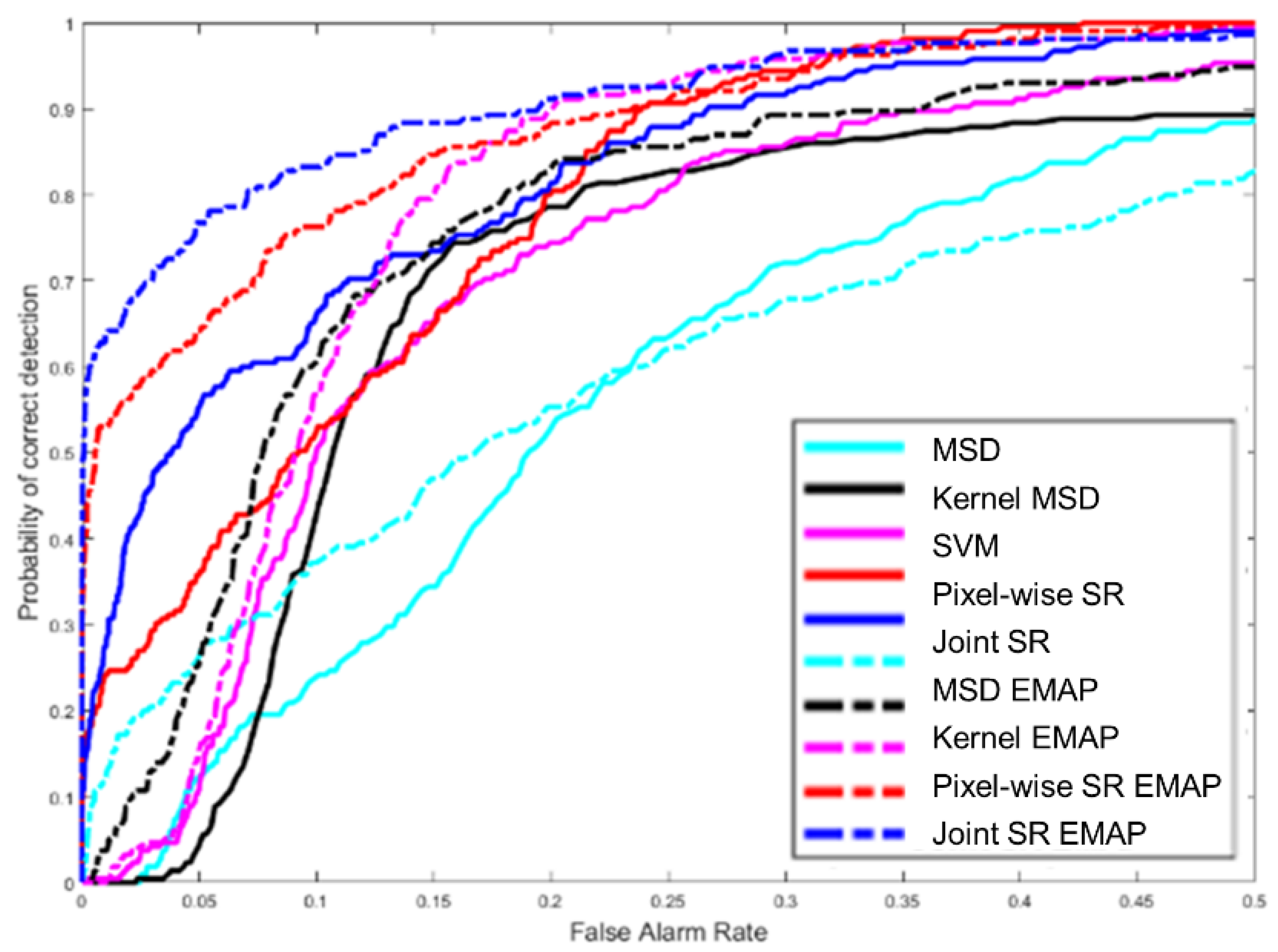
Here, rather than explaining the details of EMAP, we would like to demonstrate the advantages of EMAP for soil detection. There are eight MS bands in Worldview-3 images. We generated 80 synthetic bands using EMAP. Soil detection was then carried out using the combined 80 synthetic bands and 8 MS bands. Figure 9 shows the performance using color images for soil detection. It can be seen that the performance was poor. None of the detection methods (MSD [119], kernel MSD [120], SVM [121], and Orthogonal Matching Pursuit (OMP) or (JSR) [12] worked well. In contrast, Figure 10 [37,38] shows the results of using synthetic HS images with 88 bands for soil detection. It can be seen that the performance improvement from using synthetic bands is very significant. For example, at a 5% false alarm rate (FAR), the correct detection rate was improved by close to 20% using the joint sparsity method. More details can be found in [37,38].

3.5. Possibility of Change Detection Using Temporally-Fused Images

Here, we consider an interesting application scenario. At time t1, we have one HR MS image and a LR MS image. However, at time t2, we only have a LR MS image. We would like to ask two questions. First, can we somehow use the aforementioned images and synthesize a HR MS image at t2? Second, can we perform change detection using the HR MS image at t1 and the synthesized HR MS image at t2?
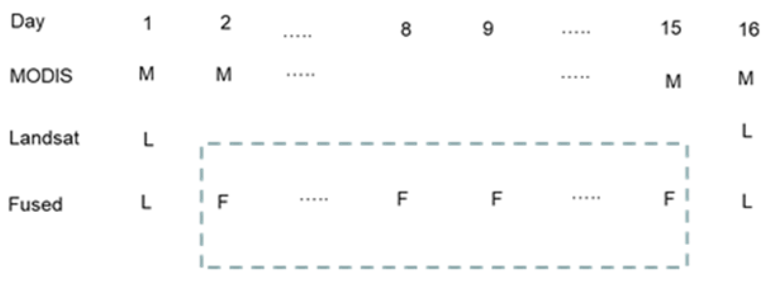
Such scenarios do exist. As shown in Figure 11, one example is the fusion of Landsat (30 m spatial resolution with 16-day revisit period) and MODIS (500 m spatial resolution with almost daily revisit). More details can be found in [148,149]. Another application scenario is the fusion of Worldview with Planet images [40]. A third temporal fusion study is for Landsat and Worldview images [150]. Once the fused images are available, more frequent change detection can then be performed for a given area. However, one limiting factor for change detection performance is the fusion performance.
A paper by Xu et al. [151] discusses a change detection approach that uses synthetically-generated images. A sparsity-based approach is used to learn the mapping between a pair of fine and coarse images. The learned mapping is then applied to the coarse image at a later time to produce a fine resolution image. Change detection is then performed between the synthetic image and the earlier fine image. The authors compared their approach with STARFM and observed that the performance was better.

3.6. Possibility of Change Detection Using Multimodal Images

As mentioned earlier, there are some recent advances [63,64,65,66,67,152,153] in change detection using multimodal or heterogeneous images. However, more research is still needed to yield consistent results.

4. Conclusions

There are many successful remote sensing applications using MS and HS images; change detection is one of them. However, there are still some challenging problems in change detection that need to be addressed. In this paper, we review some of the best known and most representative change detection algorithms in the literature. Their advantages and disadvantages are highlighted. Some recent advances in change detection using multimodal images are also mentioned. It is also worth mentioning one deep-learning approach [99] that does not require training data. We think that this approach is quite promising. We then focus on some challenging problems in change detection from a practitioner’s viewpoint. For instance, the registration of two images collected at different times may be considered a solved problem. However, in practice, this is far from the truth, especially for non-nadir images such as Worldview images. Other challenges include the use of enhanced images for change detection, and the use of fused images to increase the temporal resolution of images, etc. Some problems persist, and more research is needed.

Funding

This research received no external funding.

Acknowledgments

C.K. would like to thank all the anonymous reviewers for their comments and suggestions, which greatly improved the quality of this paper.

Conflicts of Interest

The author declares no conflict of interest.

References

  1. Landsat Bands. Available online: https://www.usgs.gov/media/images/landsat-8-band-designations (accessed on 5 August 2019).
  2. Kwan, C.; Budavari, B.; Bovik, A.C.; Marchisio, G. Blind Quality Assessment of Fused WorldView-3 Images by Using the Combinations of Pansharpening and Hypersharpening Paradigms. IEEE Geosci. Remote Sens. Lett. 2017, 14, 1835–1839. [Google Scholar] [CrossRef]
  3. Kwan, C.; Choi, J.H.; Chan, S.H.; Zhou, J.; Budavari, B. A Super-Resolution and Fusion Approach to Enhancing Hyperspectral Images. Remote Sens. 2018, 10, 1416. [Google Scholar] [CrossRef]
  4. Ayhan, B.; Kwan, C.; Jensen, J.O. Remote vapor detection and classification using hyperspectral images. In Chemical, Biological, Radiological, Nuclear, and Explosives (CBRNE) Sensing XX; SPIE: Bellingham, WA, USA, 2019; Volume 110100U. [Google Scholar]
  5. Dao, M.; Kwan, C.; Ayhan, B.; Tran, T. Burn Scar Detection Using Cloudy MODIS Images via Low-rank and Sparsity-based Models. In Proceedings of the IEEE Global Conference on Signal. and Information Processing, Washington, DC, USA, 7–9 December 2016; pp. 177–181. [Google Scholar]
  6. Wang, W.; Li, S.; Qi, H.; Ayhan, B.; Kwan, C.; Vance, S. Identify Anomaly Component by Sparsity and Low Rank. In Proceedings of the IEEE Workshop on Hyperspectral Image and Signal. Processing: Evolution in Remote Sensor (WHISPERS), Tokyo, Japan, 2–5 June 2015. [Google Scholar]
  7. Chang, C.I. Hyperspectral Imaging; Springer: Berlin, Germany, 2003. [Google Scholar]
  8. Li, S.; Wang, W.; Qi, H.; Ayhan, B.; Kwan, C.; Vance, S. Low-rank Tensor Decomposition based Anomaly Detection for Hyperspectral Imagery. In Proceedings of the IEEE International Conference on Image Processing (ICIP), Quebec City, QC, Canada, 27–30 September 2015; pp. 4525–4529. [Google Scholar]
  9. Qu, Y.; Guo, R.; Wang, W.; Qi, H.; Ayhan, B.; Kwan, C.; Vance, S. Anomaly Detection in Hyperspectral Images Through Spectral Unmixing and Low Rank Decomposition. In Proceedings of the IEEE International Geoscience and Remote Sensing Symposium (IGARSS), Beijing, China, 10–15 July 2016; pp. 1855–1858. [Google Scholar]
  10. Qu, Y.; Qi, H.; Ayhan, B.; Kwan, C.; Kidd, R. Does Multispectral/Hyperspectral Pansharpening Improve the Performance of Anomaly Detection? In Proceedings of the IEEE International Geoscience and Remote Sensing Symposium (IGARSS), Fort Worth, TX, USA, 23–28 June 2017; pp. 6130–6133. [Google Scholar]
  11. Kwan, C.; Ayhan, B.; Chen, G.; Chang, C.; Wang, J.; Ji, B. A Novel Approach for Spectral Unmixing, Classification, and Concentration Estimation of Chemical and Biological Agents. IEEE Trans. Geosci. Remote Sens. 2006, 44, 409–419. [Google Scholar] [CrossRef]
  12. Dao, M.; Kwan, C.; Koperski, K.; Marchisio, G. A Joint Sparsity Approach to Tunnel Activity Monitoring Using High Resolution Satellite Images. In Proceedings of the IEEE Ubiquitous Computing, Electronics & Mobile Communication Conference, New York, NY, USA, 19–21 October 2017; pp. 322–328. [Google Scholar]
  13. Zhou, J.; Kwan, C.; Ayhan, B. Improved Target Detection for Hyperspectral Images Using Hybrid In-Scene Calibration. J. Appl. Remote Sens. 2017, 11, 035010. [Google Scholar] [CrossRef]
  14. Ayhan, B.; Kwan, C. Application of Deep Belief Network to Land Classification Using Hyperspectral Images. In Proceedings of the 14th International Symposium on Neural Networks, Hokkaido, Japan, 21–26 June 2017; pp. 269–276. [Google Scholar]
  15. Kwan, C.; Ayhan, B. Automatic Target Recognition System with Online Machine Learning Capability. U.S. Patent 9940520, 10 April 2018. [Google Scholar]
  16. Zhou, J.; Kwan, C.; Ayhan, B.; Eismann, M. A Novel Cluster Kernel RX Algorithm for Anomaly and Change Detection Using Hyperspectral Images. IEEE Trans. Geosci. Remote Sens. 2016, 54, 6497–6504. [Google Scholar] [CrossRef]
  17. Kwan, C.; Chou, B.; Hagen, L.; Perez, D.; Li, J.; Shen, Y.; Koperski, K. Change Detection using Landsat and Worldview Images. In Algorithms, Technologies, and Applications for Multispectral and Hyperspectral Imagery XXV (Conference SI109); SPIE: Bellingham, WA, USA, 2019. [Google Scholar]
  18. Lee, C.M.; Cable, M.L.; Hook, S.J.; Green, R.O.; Ustin, S.L.; Mandl, D.J.; Middleton, E.M. An introduction to the NASA hyperspectral infrared imager (HyspIRI) mission and preparatory activities. Remote Sens. Environ. 2015, 167, 6–19. [Google Scholar] [CrossRef]
  19. Kwan, C. Image Resolution Enhancement for Remote Sensing Applications. In Proceedings of the 2nd International Conference on Vision, Image and Signal Processing, Las Vegas, CA, USA, 27–29 August 2018. [Google Scholar]
  20. Kwan, C.; Choi, J.H.; Chan, S.; Zhou, J.; Budavari, B. Resolution Enhancement for Hyperspectral Images: A Super-Resolution and Fusion Approach. In Proceedings of the IEEE International Conference on Acoustics, Speech, and Signal Processing, New Orleans, LA, USA, 5–9 March 2017; pp. 6180–6184. [Google Scholar]
  21. Loncan, L.; de Almeida, L.B.; Bioucas-Dias, J.M.; Briottet, X.; Chanussot, J.; Dobigeon, N.; Fabre, S.; Liao, W.; Licciardi, G.A.; Simoes, M. Hyperspectral pansharpening: A review. IEEE Geosci. Remote Sens. Mag. 2015, 3, 27–46. [Google Scholar] [CrossRef]
  22. Vivone, G.; Alparone, L.; Chanussot, J.; Dalla Mura, M.; Garzelli, A.; Licciardi, G.A.; Restaino, R.; Wald, L. A critical comparison among pansharpening algorithms. IEEE Trans. Geosci. Remote Sens. 2015, 53, 2565–2586. [Google Scholar] [CrossRef]
  23. Radke, R.J.; Andra, S.; Al-Kofani, O.; Roysam, B. Image change detection algorithms: A systematic survey. IEEE Trans. Image Proc. 2005, 14, 294–307. [Google Scholar] [CrossRef]
  24. Unsalan, C.; Boyer, K.L. Multispectral Satellite Image Understanding; Springer: Berlin, Germany, 2011. [Google Scholar]
  25. İlsever, M.; Unsalan, C. Two-Dimensional Change Detection Methods; Springer: Berlin, Germany, 2012. [Google Scholar]
  26. Bovolo, F.; Bruzzone, L. The time variable in data fusion: A change detection perspective. IEEE Geosci. Remote Sens. Mag. 2015, 3, 8–26. [Google Scholar] [CrossRef]
  27. Perez, D.; Banerjee, D.; Kwan, C.; Dao, M.; Shen, Y.; Koperski, K.; Marchisio, G.; Li, J. Deep Learning for Effective Detection of Excavated Soil Related to Illegal Tunnel Activities. In Proceedings of the IEEE Ubiquitous Computing, Electronics & Mobile Communication Conference, New York, NY, USA, 19–21 October 2017; pp. 626–632. [Google Scholar]
  28. Lu, Y.; Perez, D.; Dao, M.; Kwan, C.; Li, J. Deep Learning with Synthetic Hyperspectral Images for Improved Soil Detection in Multispectral Imagery. In Proceedings of the IEEE Ubiquitous Computing, Electronics & Mobile Communication Conference, New York, NY, USA, 8–10 November 2018. [Google Scholar]
  29. Kwan, C.; Chou, B.; Hagen, L.; Yang, J.; Ayhan, B.; Koperski, K. Ground Object Detection Using Worldview Images. In Signal Processing, Sensor/Information Fusion, and Target Recognition XXVIII; SPIE: Bellingham, WA, USA, 2019. [Google Scholar]
  30. Kwan, C.; Ayhan, B.; Budavari, B. Fusion of THEMIS and TES for Accurate Mars Surface Characterization. In Proceedings of the IEEE International Geoscience Remote Sensing Symposium (IGARSS), Fort Worth, TX, USA, 23–18 July 2017; pp. 3381–3384. [Google Scholar]
  31. Kwan, C.; Haberle, C.; Ayhan, B.; Chou, B.; Echavarren, A.; Castaneda, G.; Budavari, B.; Dickenshied, S. On the Generation of High-Spatial and High-Spectral Resolution Images Using THEMIS and TES for Mars Exploration. In Algorithms and Technologies for Multispectral, Hyperspectral, and Ultraspectral Imagery XXIV; SPIE: Bellingham, WA, USA, 2018; Volume 106440B. [Google Scholar]
  32. Dao, M.; Kwan, C.; Ayhan, B.; Bell, J.F. Enhancing Mastcam Images for Mars Rover Mission. In Proceedings of the 14th International Symposium on Neural Networks, Hokkaido, Japan, 21–26 June 2017; pp. 197–206. [Google Scholar]
  33. Kwan, C.; Budavari, B.; Dao, M.; Ayhan, B.; Bell, J.F. Pansharpening of Mastcam images. In Proceedings of the IEEE International Geoscience and Remote Sensing Symposium (IGARSS), Fort Worth, TX, USA, 23–28 July 2017; pp. 5117–5120. [Google Scholar]
  34. Ayhan, B.; Dao, M.; Kwan, C.; Chen, H.; Bell, J.F.; Kidd, R. A Novel Utilization of Image Registration Techniques to Process Mastcam Images in Mars Rover with Applications to Image Fusion, Pixel Clustering, and Anomaly Detection. IEEE J. Sel. Top. Appl. Earth Obs. Remote Sens. 2017, 10, 4553–4564. [Google Scholar] [CrossRef]
  35. Kwan, C.; Chou, B.; Ayhan, B. Enhancing Stereo Image Formation and Depth Map Estimation for Mastcam Images. In Proceedings of the IEEE Ubiquitous Computing, Electronics & Mobile Communication Conference, New York, NY, USA, 8–10 November 2018. [Google Scholar]
  36. Kwan, C.; Chou, B.; Ayhan, B. Stereo Image and Depth Map Generation for Images with Different Views and Resolutions. In Proceedings of the IEEE Ubiquitous Computing, Electronics & Mobile Communication Conference, New York, NY, USA, 8–10 November 2018. [Google Scholar]
  37. Dao, M.; Kwan, C.; Garcia, S.B.; Plaza, A.; Koperski, K. A New Approach to Soil Detection Using Expanded Spectral Bands. IEEE Geosci. Remote Sens. Lett. 2019. [Google Scholar] [CrossRef]
  38. Kwan, C. Remote Sensing Performance Enhancement in Hyperspectral Images. Sensors 2018, 18, 3598. [Google Scholar] [CrossRef] [PubMed]
  39. Zanetti, M.; Bovolo, F.; Bruzzone, L. Rayleigh-Rice mixture parameter estimation via EM algorithm for change detection in multispectral images. IEEE Trans. Image Proc. 2015, 24, 5004–5016. [Google Scholar] [CrossRef] [PubMed]
  40. Kwan, C.; Zhu, X.; Gao, F.; Chou, B.; Perez, D.; Li, J.; Shen, Y.; Koperski, K.; Marchisio, G. Assessment of Spatiotemporal Fusion Algorithms for Worldview and Planet Images. Sensors 2018, 18, 1051. [Google Scholar] [CrossRef]
  41. Liu, S.; Bruzzone, L.; Bovolo, F.; Zanetti, M.; Du, P. Sequential Spectral Change Vector Analysis for Change Detection in Multitemporal Hyperspectral Images. IEEE Trans. Geosci. Remote Sens. 2015, 53, 4363–4378. [Google Scholar] [CrossRef]
  42. Euclidean Distance: Raw, Normalized, and Double-Scaled Coefficients. Available online: https://www.pbarrett.net/techpapers/euclid.pdf (accessed on 25 March 2019).
  43. Perez, D.; Lu, Y.; Kwan, C.; Shen, Y.; Koperski, K.; Li, J. Combining Satellite Images with Feature Indices for Improved Change Detection. In Proceedings of the IEEE Ubiquitous Computing, Electronics & Mobile Communication Conference, New York, NY, USA, 8–10 November 2018. [Google Scholar]
  44. Gao, J. Digital Analysis of Remotely Sensed Imagery; McGraw Hill Company: New York, NY, USA, 2009. [Google Scholar]
  45. Ayhan, B.; Kwan, C.; Zhou, J. A New Nonlinear Change Detection Approach Based on Band Ratioing. In Proceedings SPIE 10644, Algorithms and Technologies for Multispectral, Hyperspectral, and Ultraspectral Imagery XXIV; SPIE: Bellingham, WA, USA, 2018; Volume 1064410. [Google Scholar]
  46. Eismann, M. Hyperspectral Remote Sensing; SPIE: Bellingham, WA, USA, 2012; Volume PM210. [Google Scholar]
  47. Schaum, A. Local Covariance Equalization of Hyperspectral Imagery: Advantages and Limitations for Target Detection. In Proceedings of the IEEE Aerospace Conference, Big Sky, MT, USA, 6–13 March 2004. [Google Scholar]
  48. Schaum, A.; Stocker, A. Long-interval chronochrome target detection. In Proceedings of the International Symposium on Spectral Sensing Research, San Diego, CA, USA, 14–19 December 1997. [Google Scholar]
  49. Zhou, J.; Ayhan, B.; Kwan, C.; Eismann, M. New and Fast algorithms for Anomaly and Change Detection in Hyperspectral images. In Proceedings of the International Symposium on Spectral Sensing Research, Springfield, MO, USA, 21–24 June 2010. [Google Scholar]
  50. Eismann, M.T.; Meola, J.; Hardie, R.C. Hyperspectral change detection in the presence of diurnal and seasonal variations. IEEE Trans. Geosci. Remote Sens. 2008, 46, 237–249. [Google Scholar] [CrossRef]
  51. Reed, I.S.; Yu, X. Adaptive multiple-band CFAR detection of an optical pattern with unknown spectral distribution. IEEE Trans. Acoust. Speech Signal Process. 1990, 38, 1760–1770. [Google Scholar] [CrossRef]
  52. Kwon, H.; Nasrabadi, N.M. Kernel RX-algorithm: A nonlinear anomaly detector for hyperspectral imagery. IEEE Trans. Geosci. Remote Sens. 2005, 43, 388–397. [Google Scholar] [CrossRef]
  53. Zhao, C.; Deng, W.; Yan, Y.; Yao, X. Progressive Line Processing of Kernel RX Anomaly Detection Algorithm for Hyperspectral Imagery. Sensors 2017, 17, 1815. [Google Scholar] [CrossRef]
  54. Qu, Y.; Wang, W.; Guo, R.; Ayhan, B.; Kwan, C.; Vance, S.; Qi, H. Hyperspectral Anomaly Detection Through Spectral Unmixing and Dictionary-Based Low-Rank Decomposition. IEEE Trans. Geosci. Remote Sens. 2018, 56, 4391–4405. [Google Scholar] [CrossRef]
  55. Zhou, J.; Kwan, C. High Performance Change Detection in Hyperspectral Images Using Multiple References. In Proceedings of the SPIE Defense + Security Conference, Anaheim, CA, USA, 15–19 April 2018. [Google Scholar]
  56. Ruff, S.W.; Christensen, P.R. Bright and dark regions on Mars: Particle size and mineralogical characteristics based on Thermal Emission Spectrometer data. J. Geogr. Res. Planets 2002, 107. [Google Scholar] [CrossRef]
  57. Li, X.; Zhao, S.; Yang, H.; Cong, D.; Zhang, Z. A Bi-Band Binary Mask Based Land-Use Change Detection Using Landsat 8 OLI Imagery. Sustainability 2017, 9, 479. [Google Scholar] [CrossRef]
  58. Xu, Y.; Xiang, S.; Huo, C.; Pan, C. Change Detection Based on Auto-encoder Model for VHR Images. In SPIE MIPPR (2013): Pattern Recognition and Computer Vision, Proceedings of the 8th International Symposium on Multispectral Image Processing and Pattern Recognition, Wuhan, China, 26–27 October 2013; Cao, Z., Ed.; SPIE: Bellingham, WA, USA, 2013; p. 8919. [Google Scholar]
  59. Wu, C.; Du, B.; Zhang, L. Hyperspectral anomalous change detection based on joint sparse representation. ISPRS J. Photogramm. Remote Sens. 2018, 146, 137–150. [Google Scholar] [CrossRef]
  60. Zanetti, M.; Bruzzone, L. A theoretical framework for change detection based on a compound multiclass statistical model of the difference image. IEEE Trans. Geosci. Remote Sens. 2018, 56, 1129–1143. [Google Scholar] [CrossRef]
  61. Falco, N.; Mura, M.D.; Bovolo, F.; Benediktsson, J.A.; Bruzzone, L. Change detection in VHR images based on morphological attribute profiles. IEEE Geosci. Remote Sensing Lett. 2013, 10, 636–640. [Google Scholar] [CrossRef]
  62. Touati, R.; Mignotte, M. An Energy-Based Model Encoding Nonlocal Pairwise Pixel Interactions for Multisensor Change Detection. IEEE Trans. Geosci. Remote Sens. 2018, 56, 1046–1058. [Google Scholar] [CrossRef]
  63. Gong, M.; Zhang, P.; Su, L.; Liu, J. Coupled dictionary learning for change detection from multisource data. IEEE Trans. Geosci. Remote Sens. 2016, 54, 7077–7091. [Google Scholar] [CrossRef]
  64. Ziemann, A.K.; Theiler, J. Multi-sensor anomalous change detection at scale. In Proceedings of the SPIE Conference Algorithms, Technologies, and Applications for Multispectral and Hyperspectral Imagery XXV, Baltimore, MD, USA, 26–30 April 2019. [Google Scholar]
  65. Liu, Z.; Li, G.; Mercier, G.; He, Y.; Pan, Q. Change Detection in Heterogeneous Remote Sensing Images via Homogeneous Pixel Transformation. IEEE Trans. Image Proc. 2018, 27, 1822–1834. [Google Scholar] [CrossRef]
  66. Zhan, T.; Gong, M.; Jiang, X.; Li, S. Log-Based Transformation Feature Learning for Change Detection in Heterogeneous Images. IEEE Geosci. Remote Sens. Lett. 2018, 15, 1352–1356. [Google Scholar] [CrossRef]
  67. Tan, K.; Jin, X.; Plaza, A.; Wang, X.; Xiao, L.; Du, P. Automatic Change Detection in High-Resolution Remote Sensing Images by Using a Multiple Classifier System and Spectral–Spatial Features. IEEE J. Sel. Top. Appl. Earth Obs. Remote Sens. 2016, 9, 3439–3451. [Google Scholar] [CrossRef]
  68. Wang, X.; Liu, S.; Du, P.; Liang, H.; Xia, J.; Li, Y. Object-Based Change Detection in Urban Areas from High Spatial Resolution Images Based on Multiple Features and Ensemble Learning. Remote Sens. 2018, 10, 276. [Google Scholar] [CrossRef] [Green Version]
  69. Huo, C.; Chen, K.; Ding, K.; Zhou, Z.; Pan, C. Learning relationship for very high resolution image change detection. IEEE J. Sel. Top. App. Earth Obs. Remote Sens. 2016, 9, 3384–3394. [Google Scholar] [CrossRef]
  70. Wu, C.; Zhang, L.; Du, B. Kernel Slow Feature Analysis for Scene Change Detection. IEEE Trans. Geosci. Remote Sens. 2017, 55, 2367–2384. [Google Scholar] [CrossRef]
  71. Zhang, W.; Lu, X.; Li, X. A Coarse-to-Fine Semi-Supervised Change Detection for Multispectral Images. IEEE Trans. Geosci. Remote Sens. 2018, 56, 3587–3599. [Google Scholar] [CrossRef]
  72. Chen, Q.; Chen, Y.; Jiang, W. Genetic Particle Swarm Optimization–Based Feature Selection for Very-High-Resolution Remotely Sensed Imagery Object Change Detection. Sensors 2016, 16, 1204. [Google Scholar] [CrossRef] [Green Version]
  73. Hou, B.; Wang, Y.; Liu, Q. A Saliency Guided Semi-Supervised Building Change Detection Method for High Resolution Remote Sensing Images. Sensors 2016, 16, 1377. [Google Scholar] [CrossRef] [Green Version]
  74. Yu, H.; Yang, W.; Hua, G.; Ru, H.; Huang, P. Change Detection Using High Resolution Remote Sensing Images Based on Active Learning and Markov Random Fields. Remote Sens. 2017, 9, 1233. [Google Scholar] [CrossRef] [Green Version]
  75. Feng, W.; Sui, H.; Tu, J.; Huang, W.; Xu, C.; Sun, K. A Novel Change Detection Approach for Multi-Temporal High-Resolution Remote Sensing Images Based on Rotation Forest and Coarse-to-Fine Uncertainty Analyses. Remote Sens. 2018, 10, 1015. [Google Scholar] [CrossRef] [Green Version]
  76. Tan, K.; Zhang, Y.; Wang, X.; Chen, Y. Object-Based Change Detection Using Multiple Classifiers and Multi-Scale Uncertainty Analysis. Remote Sens. 2019, 11, 359. [Google Scholar] [CrossRef] [Green Version]
  77. Chen, Z.; Wang, B. Spectrally-Spatially Regularized Low-Rank and Sparse Decomposition: A Novel Method for Change Detection in Multitemporal Hyperspectral Images. Remote Sens. 2017, 9, 1044. [Google Scholar] [CrossRef] [Green Version]
  78. Erturk, A.; Iordache, M.-D.; Plaza, A. Sparse Unmixing With Dictionary Pruning for Hyperspectral Change Detection. IEEE J. Sel. Top. Appl. Earth Obs. Remote Sens. 2017, 10, 321–330. [Google Scholar] [CrossRef]
  79. Wu, K.; Du, Q.; Wang, Y.; Yang, Y. Supervised Sub-Pixel Mapping for Change Detection from Remotely Sensed Images with Different Resolutions. Remote Sens. 2017, 9, 284. [Google Scholar] [CrossRef] [Green Version]
  80. Zhang, W.; Lu, X. The Spectral-Spatial Joint Learning for Change Detection in Multispectral Imagery. Remote Sens. 2019, 11, 240. [Google Scholar] [CrossRef] [Green Version]
  81. Wang, Q.; Yuan, Z.; Du, Q.; Li, X. GETNET: A General End-to-End 2-D CNN Framework for Hyperspectral Image Change Detection. IEEE Trans. Geosci. Remote Sens. 2019, 57, 3–13. [Google Scholar] [CrossRef] [Green Version]
  82. Lyu, H.; Lu, H.; Mou, L. Learning a Transferable Change Rule from a Recurrent Neural Network for Land Cover Change Detection. Remote Sens. 2016, 8, 506. [Google Scholar] [CrossRef] [Green Version]
  83. Song, A.; Choi, J.; Han, Y.; Kim, Y. Change Detection in Hyperspectral Images Using Recurrent 3D Fully Convolutional Networks. Remote Sens. 2018, 10, 1827. [Google Scholar] [CrossRef] [Green Version]
  84. Ma, W.; Xiong, Y.; Wu, Y.; Yang, H.; Zhang, X.; Jiao, L. Change Detection in Remote Sensing Images Based on Image Mapping and a Deep Capsule Network. Remote Sens. 2019, 11, 626. [Google Scholar] [CrossRef] [Green Version]
  85. Liu, S.; Bruzzone, L.; Bovolo, F.; Du, P. Hierarchical Unsupervised Change Detection in Multitemporal Hyperspectral Images. IEEE Trans. Geosci. Remote Sens. 2015, 53, 244–260. [Google Scholar]
  86. Zhuang, H.; Deng, K.; Fan, H.; Yu, M. Strategies Combining Spectral Angle Mapper and Change Vector Analysis to Unsupervised Change Detection in Multispectral Images. IEEE Geosci. Remote Sens. Lett. 2016, 13, 681–685. [Google Scholar] [CrossRef]
  87. Liu, S.; Bruzzone, L.; Bovolo, F.; Du, P. Unsupervised Multitemporal Spectral Unmixing for Detecting Multiple Changes in Hyperspectral Images. IEEE Trans. Geosci. Remote Sens. 2016, 54, 2733–2748. [Google Scholar] [CrossRef]
  88. Shah-Hosseini, R.; Homayouni, S.; Safari, A. A Hybrid Kernel-Based Change Detection Method for Remotely Sensed Data in a Similarity Space. Remote Sens. 2015, 7, 12829–12858. [Google Scholar] [CrossRef] [Green Version]
  89. Shao, P.; Shi, W.; He, P.; Hao, M.; Zhang, X. Novel Approach to Unsupervised Change Detection Based on a Robust Semi-Supervised FCM Clustering Algorithm. Remote Sens. 2016, 8, 264. [Google Scholar] [CrossRef] [Green Version]
  90. Ma, L.; Li, M.; Blaschke, T.; Ma, X.; Tiede, D.; Cheng, L.; Chen, Z.; Chen, D. Object-Based Change Detection in Urban Areas: The Effects of Segmentation Strategy, Scale, and Feature Space on Unsupervised Methods. Remote Sens. 2016, 8, 761. [Google Scholar] [CrossRef] [Green Version]
  91. Liu, Q.; Liu, L.; Wang, Y. Unsupervised Change Detection for Multispectral Remote Sensing Images Using Random Walks. Remote Sens. 2017, 9, 438. [Google Scholar] [CrossRef] [Green Version]
  92. Wang, B.; Choi, J.; Choi, S.; Lee, S.; Wu, P.; Gao, Y. Image Fusion-Based Land Cover Change Detection Using Multi-Temporal High-Resolution Satellite Images. Remote Sens. 2017, 9, 804. [Google Scholar] [CrossRef] [Green Version]
  93. Liu, S.; Du, Q.; Tong, X.; Samat, A.; Pan, H.; Ma, X. Band Selection-Based Dimensionality Reduction for Change Detection in Multi-Temporal Hyperspectral Images. Remote Sens. 2017, 9, 1008. [Google Scholar] [CrossRef] [Green Version]
  94. Lv, Z.; Liu, T.; Wan, Y.; Benediktsson, J.A.; Zhang, X. Post-Processing Approach for Refining Raw Land Cover Change Detection of Very High-Resolution Remote Sensing Images. Remote Sens. 2018, 10, 472. [Google Scholar] [CrossRef] [Green Version]
  95. Solano-Correa, Y.T.; Bovolo, F.; Bruzzone, L. An Approach for Unsupervised Change Detection in Multitemporal VHR Images Acquired by Different Multispectral Sensors. Remote Sens. 2018, 10, 533. [Google Scholar] [CrossRef] [Green Version]
  96. Yan, L.; Xia, W.; Zhao, Z.; Wang, Y. A Novel Approach to Unsupervised Change Detection Based on Hybrid Spectral Difference. Remote Sens. 2018, 10, 841. [Google Scholar] [CrossRef] [Green Version]
  97. Park, H.; Choi, J.; Park, W.; Park, H. Modified S2CVA Algorithm Using Cross-Sharpened Images for Unsupervised Change Detection. Sustainability 2018, 10, 3301. [Google Scholar] [CrossRef] [Green Version]
  98. Lei, T.; Xue, D.; Lv, Z.; Li, S.; Zhang, Y.; Nandi, A.K. Unsupervised Change Detection Using Fast Fuzzy Clustering for Landslide Mapping from Very High-Resolution Images. Remote Sens. 2018, 10, 1381. [Google Scholar] [CrossRef] [Green Version]
  99. Li, X.; Yuan, Z.; Wang, Q. Unsupervised Deep Noise Modeling for Hyperspectral Image Change Detection. Remote Sens. 2019, 11, 258. [Google Scholar] [CrossRef] [Green Version]
  100. Mandanici, E.; Bitelli, G. Multi-Image and Multi-Sensor Change Detection for Long-Term Monitoring of Arid Environments with Landsat Series. Remote Sens. 2015, 7, 14019–14038. [Google Scholar] [CrossRef] [Green Version]
  101. Misbari, S.; Hashim, M. Change Detection of Submerged Seagrass Biomass in Shallow Coastal Water. Remote Sens. 2016, 8, 200. [Google Scholar] [CrossRef] [Green Version]
  102. Liu, H.; Meng, X.; Jiang, T.; Liu, X.; Zhang, A. Change Detection of Phragmites Australis Distribution in the Detroit Wildlife Refuge Based on an Iterative Intersection Analysis Algorithm. Sustainability 2016, 8, 264. [Google Scholar] [CrossRef] [Green Version]
  103. Ballanti, L.; Byrd, K.B.; Woo, I.; Ellings, C. Remote Sensing for Wetland Mapping and Historical Change Detection at the Nisqually River Delta. Sustainability 2017, 9, 1919. [Google Scholar] [CrossRef] [Green Version]
  104. Lv, Z.; Shi, W.; Zhou, X.; Benediktsson, J.A. Semi-Automatic System for Land Cover Change Detection Using Bi-Temporal Remote Sensing Images. Remote Sens. 2017, 9, 1112. [Google Scholar] [CrossRef] [Green Version]
  105. Lv, Z.; Liu, T.; Zhang, P.; Benediktsson, J.A.; Chen, Y. Land Cover Change Detection Based on Adaptive Contextual Information Using Bi-Temporal Remote Sensing Images. Remote Sens. 2018, 10, 901. [Google Scholar] [CrossRef] [Green Version]
  106. Luo, H.; Liu, C.; Wu, C.; Guo, X. Urban Change Detection Based on Dempster–Shafer Theory for Multi-temporal Very High-Resolution Imagery. Remote Sens. 2018, 10, 980. [Google Scholar] [CrossRef] [Green Version]
  107. Liu, H.; Yang, M.; Chen, J.; Hou, J.; Deng, M. Line-Constrained Shape Feature for Building Change Detection in VHR Remote Sensing Imagery. ISPRS Int. J. Geo-Inf. 2018, 7, 410. [Google Scholar] [CrossRef] [Green Version]
  108. Zhou, Z.; Ma, L.; Fu, T.; Zhang, G.; Yao, M.; Li, M. Change Detection in Coral Reef Environment Using High-Resolution Images: Comparison of Object-Based and Pixel-Based Paradigms. ISPRS Int. J. Geo-Inf. 2018, 7, 441. [Google Scholar] [CrossRef] [Green Version]
  109. Gstaiger, V.; Tian, J.; Kiefl, R.; Kurz, F. 2D vs. 3D Change Detection Using Aerial Imagery to Support Crisis Management of Large-Scale Events. Remote Sens. 2018, 10, 2054. [Google Scholar] [CrossRef] [Green Version]
  110. Gadal, S.; Ouerghemmi, W. Multi-Level Morphometric Characterization of Built-up Areas and Change Detection in Siberian Sub-Arctic Urban Area: Yakutsk. ISPRS Int. J. Geo-Inf. 2019, 8, 129. [Google Scholar] [CrossRef] [Green Version]
  111. Bueno, I.T.; Acerbi Júnior, F.W.; Silveira, E.M.O.; Mello, J.M.; Carvalho, L.M.T.; Gomide, L.R.; Withey, K.; Scolforo, J.R.S. Object-Based Change Detection in the Cerrado Biome Using Landsat Time Series. Remote Sens. 2019, 11, 570. [Google Scholar] [CrossRef] [Green Version]
  112. Gong, J.; Hu, X.; Pang, S.; Li, K. Patch Matching and Dense CRF-Based Co-Refinement for Building Change Detection from Bi-Temporal Aerial Images. Sensors 2019, 19, 1557. [Google Scholar] [CrossRef] [Green Version]
  113. Marchesi, S.; Bovolo, F.; Bruzzone, L. A Context-Sensitive Technique Robust to Registration Noise for Change Detection in VHR Multispectral Images. IEEE Trans. Image Proc. 2010, 19, 1877–1889. [Google Scholar] [CrossRef]
  114. Vongsy, K.; Eismann, M.T.; Mendenhall, M.J. Extension of the Linear Chromodynamics Model for Spectral Change Detection in the Presence of Residual Spatial Misregistration. IEEE Trans. Geosci. Remote Sens. 2015, 53, 3005–3021. [Google Scholar] [CrossRef]
  115. Ayhan, B.; Kwan, C. On the use of Radiance Domain for Burn Scar Detection under Varying Atmospheric Illumination Conditions and Viewing Geometry. J. Signal Image Video Proc. 2016, 11, 605–612. [Google Scholar] [CrossRef]
  116. Zhou, J.; Kwan, C. Fast Anomaly Detection Algorithms for Hyperspectral Images. J. Multidiscip. Eng. Sci. Technol. 2015, 2, 2521–2525. [Google Scholar]
  117. Chang, C.-I. Real-Time Recursive Hyperspectral Sample and Band Processing; Springer: Berlin, Germany, 2017. [Google Scholar]
  118. Manolakis, D.; Siracusa, C.; Shaw, G. Adaptive Matched Subspace Detectors for Hyperspectral Imaging Applications. In Proceedings of the International Conference on Acoustics, Speech and Signal Processing, Salt Lake City, UT, USA, 7–11 May 2001. [Google Scholar]
  119. Kwan, C. Method and System for Generating High ResolutionWorldview-3 Images. U.S. Patent 10192288, 28 June 2019. [Google Scholar]
  120. Kwon, H.; Nasrabadi, N.M. Kernel matched subspace detectors for hyperspectral target detection. IEEE Trans. Pattern Anal. Mach. Intell. 2006, 28, 178–194. [Google Scholar] [CrossRef]
  121. Melgani, F.; Bruzzone, L. Classification of hyperspectral remote sensing images with support vector machines. IEEE Trans. Geosci. Remote Sens. 2004, 42, 1778–1790. [Google Scholar] [CrossRef] [Green Version]
  122. Dao, M.; Nguyen, D.; Tran, T.; Chin, S. Chemical plume detection in hyperspectral imagery via joint sparse representation. Mil. Commun. Conf. (MILCOM) 2012, 1–5. [Google Scholar] [CrossRef]
  123. Kwan, C.; Dao, M.; Chou, B.; Kwan, L.M.; Ayhan, B. Mastcam Image Enhancement Using Estimated Point Spread Functions. In Proceedings of the IEEE Ubiquitous Computing, Electronics & Mobile Communication Conference, New York, NY, USA, 19–21 October 2017. [Google Scholar]
  124. Chan, S.H.; Wang, X.; Elgendy, O.A. Plug-and-play ADMM for image restoration: Fixed point convergence and applications. IEEE Trans. Comput. Imaging 2017, 3, 84–98. [Google Scholar] [CrossRef] [Green Version]
  125. Yan, Q.; Xu, Y.; Yang, X.; Truong, T.Q. Single image superresolution based on gradient profile sharpness. IEEE Trans. Image Process. 2015, 24, 3187–3202. [Google Scholar] [PubMed]
  126. Dong, C.; Loy, C.C.; He, K.; Tang, X. Learning a deep convolutional network for image super-resolution. In Proceedings of the European Conference on Computer Vision, Zurich, Switzerland, 6–12 September 2014; pp. 184–199. [Google Scholar]
  127. Dong, C.; Loy, C.C.; Tang, X. Accelerating the super-resolution convolutional neural network. In Proceedings of the European Conference on Computer Vision, Amsterdam, The Netherlands, 8–16 October 2016; pp. 391–407. [Google Scholar]
  128. Timofte, R.; de Smet, V.; Van Gool, L. A+: Adjusted anchored neighborhood regression for fast super-resolution. In Proceedings of the Asian Conference on Computer Vision, Singapore, 1–5 November 2014; pp. 111–126. [Google Scholar]
  129. Chang, H.; Yeung, D.; Xiong, Y. Super-resolution through neighbor embedding. In Proceedings of the 2004 IEEE Computer Society Conference on Computer Vision and Pattern Recognition, Washington, DC, USA, 27 June–2 July 2004. [Google Scholar]
  130. Yokoya, N.; Yairi, T.; Iwasaki, A. Coupled nonnegative matrix factorization unmixing for hyperspectral and multispectral data fusion. IEEE Trans. Geosci. Remote Sens. 2012, 50, 528–537. [Google Scholar] [CrossRef]
  131. Hardie, R.C.; Eismann, M.T.; Wilson, G.L. Map estimation for hyperspectral image resolution enhancement using an auxiliary sensor. IEEE Trans. Image Process. 2004, 13, 1174–1184. [Google Scholar] [CrossRef] [PubMed]
  132. Wei, Q.; Bioucas-Dias, J.; Dobigeon, N.; Tourneret, J.Y. Hyperspectral and multispectral image fusion based on a sparse representation. IEEE Trans. Geosci. Remote Sens. 2015, 53, 3658–3668. [Google Scholar] [CrossRef] [Green Version]
  133. Choi, J.; Yu, K.; Kim, Y. A new adaptive component-substitution based satellite image fusion by using partial replacement. IEEE Trans. Geosci. Remote Sens. 2011, 49, 295–309. [Google Scholar] [CrossRef]
  134. Hook, S.J.; Rast, M. Mineralogic Mapping Using Airborne Visible Infrared Imaging Spectrometer (aviris), Shortwave Infrared (swir) data Acquired over Cuprite, Nevada. In Proceedings of the Second Airborne Visible Infrared Imaging Spectrometer (AVIRIS) Workshop, Pasadena, CA, USA, 4–5 June 1990; pp. 199–207. [Google Scholar]
  135. Keys, R. Cubic convolution interpolation for digital image processing. IEEE Trans. Acoust. Speech Signal Process. 1981, 29, 1153–1160. [Google Scholar] [CrossRef]
  136. Chavez, P.S., Jr.; Sides, S.C.; Anderson, J.A. Comparison of three different methods to merge multiresolution and multispectral data: Landsat tm and spot panchromatic. Photogramm. Eng. Remote Sens. 1991, 57, 295–303. [Google Scholar]
  137. Liao, W.; Huang, X.; Coillie, F.V.; Gautama, S.; Pizurica, A.; Philips, W.; Liu, H.; Zhu, T.; Shimoni, M.; Moser, G.; et al. Processing of multiresolution thermal hyperspectral and digital color data: Outcome of the 2014 IEEE GRSS data fusion contest. IEEE J. Sel. Top. Appl. Earth Obs. Remote Sens. 2015, 8, 2984–2996. [Google Scholar] [CrossRef]
  138. Laben, C.; Brower, B. Process for Enhancing the Spatial Resolution of Multispectral Imagery Using Pan-Sharpening. U.S. Patent 6011875, 4 January 2000. [Google Scholar]
  139. Aiazzi, B.; Baronti, S.; Selva, M. Improving component substitution pansharpening through multivariate regression of ms+pan data. IEEE Trans. Geosci. Remote Sens. 2007, 45, 3230–3239. [Google Scholar] [CrossRef]
  140. Aiazzi, B.; Alparone, L.; Baronti, S.; Garzelli, A.; Selva, M. MTF-tailored multiscale fusion of high-resolution ms and pan imagery. Photogramm. Eng. Remote Sens. 2006, 72, 591–596. [Google Scholar] [CrossRef]
  141. Vivone, G.; Restaino, R.; Dalla Mura, M.; Licciardi, G.; Chanussot, J. Contrast and error-based fusion schemes for multispectral image pansharpening. IEEE Geosci. Remote Sens. Lett. 2014, 11, 930–934. [Google Scholar] [CrossRef]
  142. Simoes, M.; Bioucas-Dias, J.; Almeida, L.B.; Chanussot, J. A convex formulation for hyperspectral image superresolution via subspace-based regularization. IEEE Trans. Geosci. Remote Sens. 2015, 53, 3373–3388. [Google Scholar] [CrossRef] [Green Version]
  143. Simoes, M.; Bioucas-Dias, J.; Almeida, L.B.; Chanussot, J. Hyperspectral image superresolution: An edge-preserving convex formulation. In Proceedings of the 2014 IEEE International Conference on Image Processing (ICIP), Paris, France, 27–30 October 2014; pp. 4166–4170. [Google Scholar]
  144. Liu, J.G. Smoothing filter based intensity modulation: A spectral preserve image fusion technique for improving spatial details. Int. J. Remote Sens. 2000, 21, 3461–3472. [Google Scholar] [CrossRef]
  145. Zhou, J.; Kwan, C.; Budavari, B. Hyperspectral image super-resolution: A hybrid color mapping approach. J. Appl. Remote Sens. 2016, 10, 35024. [Google Scholar] [CrossRef]
  146. Ren, H.; Chang, C.I. A generalized orthogonal subspace projection approach to unsupervised multispectral image classification. IEEE Trans. Geosci. Remote Sens. 2000, 38, 2515–2528. [Google Scholar]
  147. Bernabé, S.; Marpu, P.R.; Plaza, A.; Mura, M.D.; Benediktsson, J.A. Spectral–Spatial Classification of Multispectral Images Using Kernel Feature Space Representation. IEEE Geosci. Remote Sens. Lett. 2014, 11, 288–292. [Google Scholar] [CrossRef]
  148. Gao, F.; Masek, J.; Schwaller, M.; Hall, F. On the blending of the Landsat and MODIS surface reflectance: Predicting daily Landsat surface reflectance. IEEE Trans. Geosci. Remote Sens. 2006, 44, 2207–2218. [Google Scholar]
  149. Kwan, C.; Budavari, B.; Gao, F.; Zhu, X. A Hybrid Color Mapping Approach to Fusing MODIS and Landsat Images for Forward Prediction. Remote Sens. 2018, 10, 520. [Google Scholar] [CrossRef] [Green Version]
  150. Kwan, C.; Chou, B.; Yang, J.; Perez, D.; Shen, Y.; Li, J.; Koperski, K. Landsat and Worldview Image Fusion. In Proceedings of the Signal Processing, Sensor/Information Fusion, and Target Recognition XXVIII, Baltimore, MD, USA, 15–17 April 2019. [Google Scholar]
  151. Xu, Y.; Lin, L.; Meng, D. Learning-Based Sub-Pixel Change Detection Using Coarse Resolution Satellite Imagery. Remote Sens. 2017, 9, 709. [Google Scholar] [CrossRef] [Green Version]
  152. Kwan, C.; Ayhan, B.; Larkin, J.; Kwan, L.; Bernabé, S.; Plaza, A. Performance of change detection using heterogeneous images and Extended Multi-Attribute Profiles (EMAPs). Remote Sens. 2019, 11, 2377. [Google Scholar] [CrossRef] [Green Version]
  153. Ayhan, B.; Kwan, C. A New Approach to Change Detection Using Heterogeneous Images. In Proceedings of the IEEE 10th Annual Ubiquitous Computing, Electronics & Mobile Communication Conference, New York, NY, USA, 10–12 October 2019. [Google Scholar]
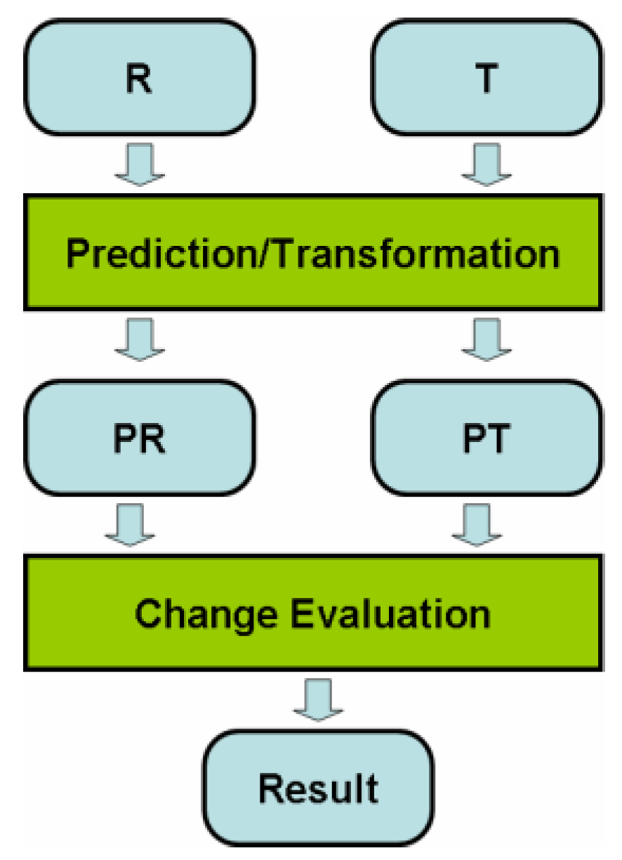
Figure 1. Change detection between two images.
Information 10 00353 g001
Figure 2. Local prediction idea.
Information 10 00353 g002
Figure 3. Residuals of global CC, segmented CC, and local CC. First row: Aug. and Oct. image pair; Second row: Sept. and Oct. image pair; Third row: Oct. and Oct. image pair; Fourth row: Nov. and Oct. image pair. Blue pixels mean small errors.
Information 10 00353 g003
Figure 4. Signal flow in MRCD.
Information 10 00353 g004
Figure 5. Block diagram of BandRatio/CC/Local RX.
Information 10 00353 g005
Figure 6. Architecture of a deep auto-encoder.
Information 10 00353 g006
Figure 7. Approach 4: A parallel pansharpening step first, followed by a sequential fusion step for enhancing WV-3 images.
Information 10 00353 g007
Figure 8. RGB and SWIR images before and after pansharpening.
Information 10 00353 g008
Figure 9. Performance of using color images for soil detection.
Information 10 00353 g009
Figure 10. Soil detection results using synthetic bands.
Information 10 00353 g010
Figure 11. Fusion of Landsat and MODIS images to create a high spatial and high temporal resolution image sequence.
Information 10 00353 g011
Table 1. Summary of recent supervised change detection methods.
Supervised MethodsReference and NotesData
Deep Learning[82] recurrent neural network (RNN)Landsat, Hyperion
[83] RNNHyperion
[84] Capsule NetworkSAR, optical
Object based[68] ensemble learningQuickbird, Ziyuan-3, Gaofen-1,
[73] Combination of pixel and object basedQuickbird
[75] Rotation forestGaofen-2
[76] Multiple classifiers (SVM, CVA, …)ZY-3
Sparsity[77] low rank and sparse representationPavia HSI, Hyperion
[78] spectral unmixingAVIRIS, APEX
[79] Sub-pixel classificationLandsat, MODIS
[80] Joint spectral-spatial learningLandsat, GF-1
[81] abundance extraction using unmixingHyperion
Others[67] Combination of conventional methodsZY-3
[69] Relationship learningQuickBird 2, Pleiades 1A
[70] Kernel Slow Feature AnalysisIKONOS
[71] Semi-automaticLandsat
[72] genetic particle swarmingWV-2, WV-3
[74] Combination of k-means and MRFWV-2
Table 2. Summary of recent unsupervised change detection algorithms.
Unsupervised MethodsReference and NotesData
Hierarchical[85] Key algorithm: CVAHyperion (hyperspectral data)
Hybrid[86] combination of CVA and SAMQuickbird
Spectral unmixing[87] change detection based on endmembersHyperion (hyperspectral data)
Kernel based[88] Utilized many clustering toolsLandsat and Quickbird
Feature based[89] Change detection using segmentation Landsat and SAR
Object based[90] Segmentation is key to successWV-2
[94] Emphasize on post-processing after object detectionAerial images and SPOT-5
Random walk[91] Combination of random walk, PCA, and GMMLandsat, ASTER, Quickbird
Image fusion based on cross-pansharpened images[92] IR-MAD for change detectionIKONOS-2, WV-3, GF-1
[97] Use modified CVAKOMPSAT-2
Band selection[93] CVA was used after band selectionHyperion
Transformation based[95] focus on features from linear transformationQuickbird, WV-2, Geoeye-1
Hybrid spectral difference[96] Combine spectral shapes, gradient of spectral shapes, and Euclidean distanceWV-2, WV-3, Landsat-7
Fuzzy clustering[98] fuzzy c-meansAerial images
Deep learning[99] UnsupervisedHyperion
Table 3. Summary of recent application-oriented change detection papers.
Reference and NotesData
Arid environment monitoring[100] NDVI for change detectionLandsat
Submerged biomass in shallow coastal water[101] substrate-leaving radiance estimationLandsat
Phragmites australis distribution[102] iterative intersection analysis algorithm based on NDVILandsat
Wetland mapping and historical change detection[103] object-based approachAerial images, WV-3 images, lidar
Land cover change detection [104] region growing algorithmAerial images, Landsat
[105] Contextual basedAerial images, Landsat
Urban change detection[106] Combined object- and pixel-based approachesGF-2 images
Building change detection[107] Object-based approachWV-2 images
[112] Patch-based approachAerial images
Coral reef change detection[108] Compared object- and pixel-based methodsQuickbird and WV-2 images
Large event crisis management[109] Compared 2D and 3D change detection methodsAerial images
Built-up area monitoring[110] supervised classification group and spectral index-based groupSentinel-2A and SPOT 6
Cerrado (Brazilian savanna) biome monitoring[111] Object based approachLandsat