
Modeling of Accidental Oil Spills at Different Phases of LNG Terminal Construction


Abstract
1. Introduction
2. Numerical Models
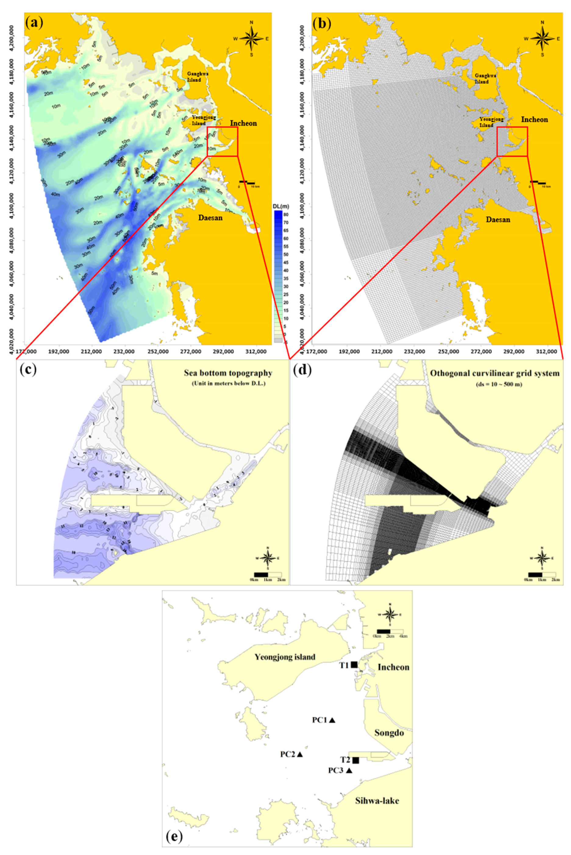
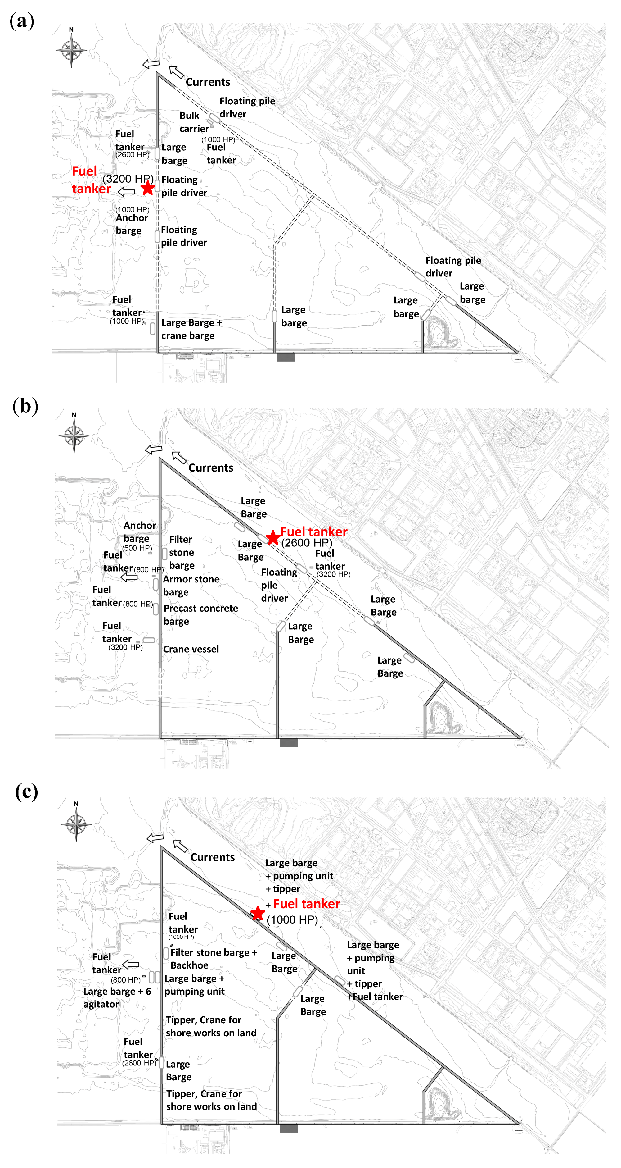
2.1. Numerical Domain and Selected Scenarios
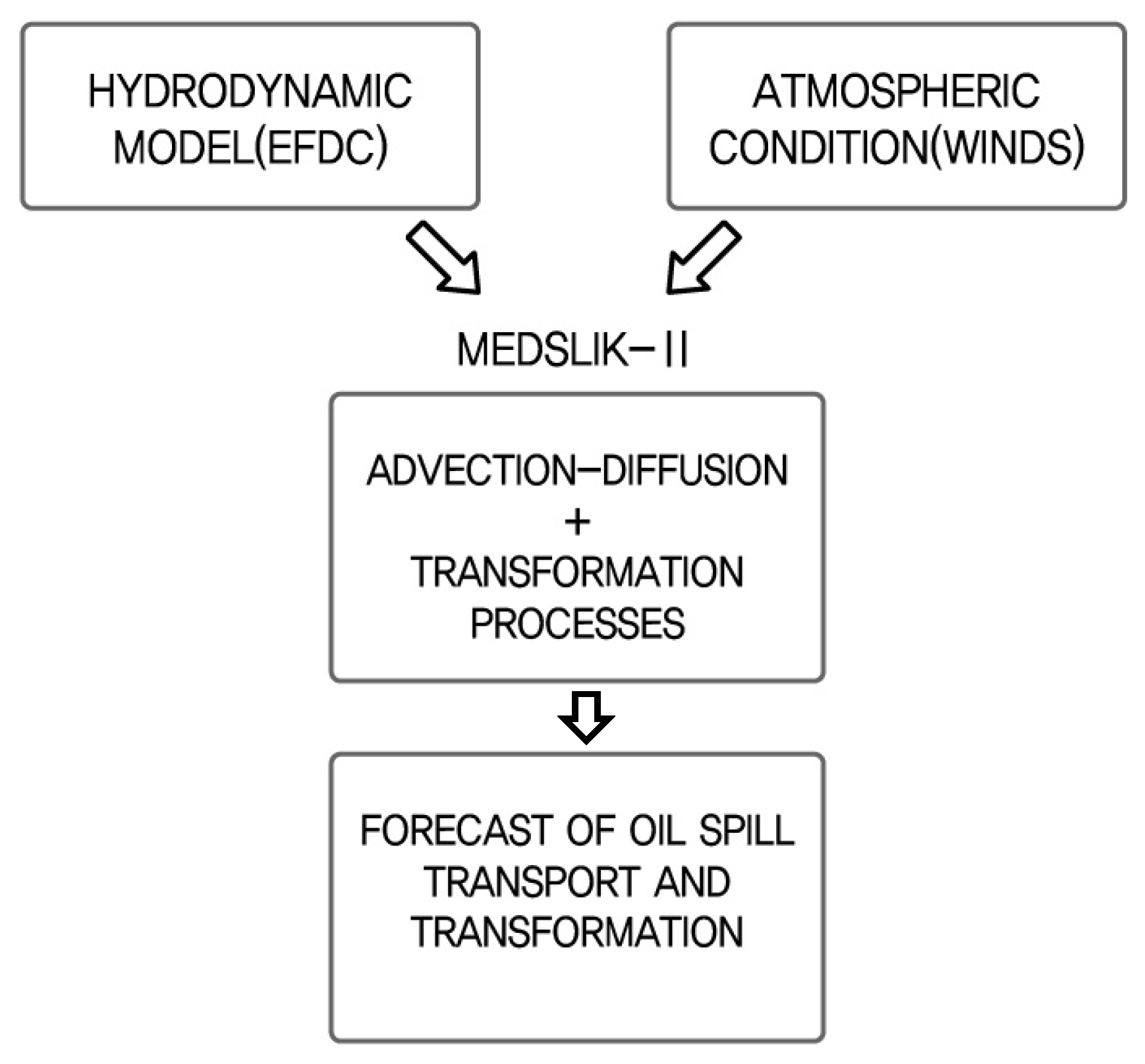
2.2. Hydrodynamic Model
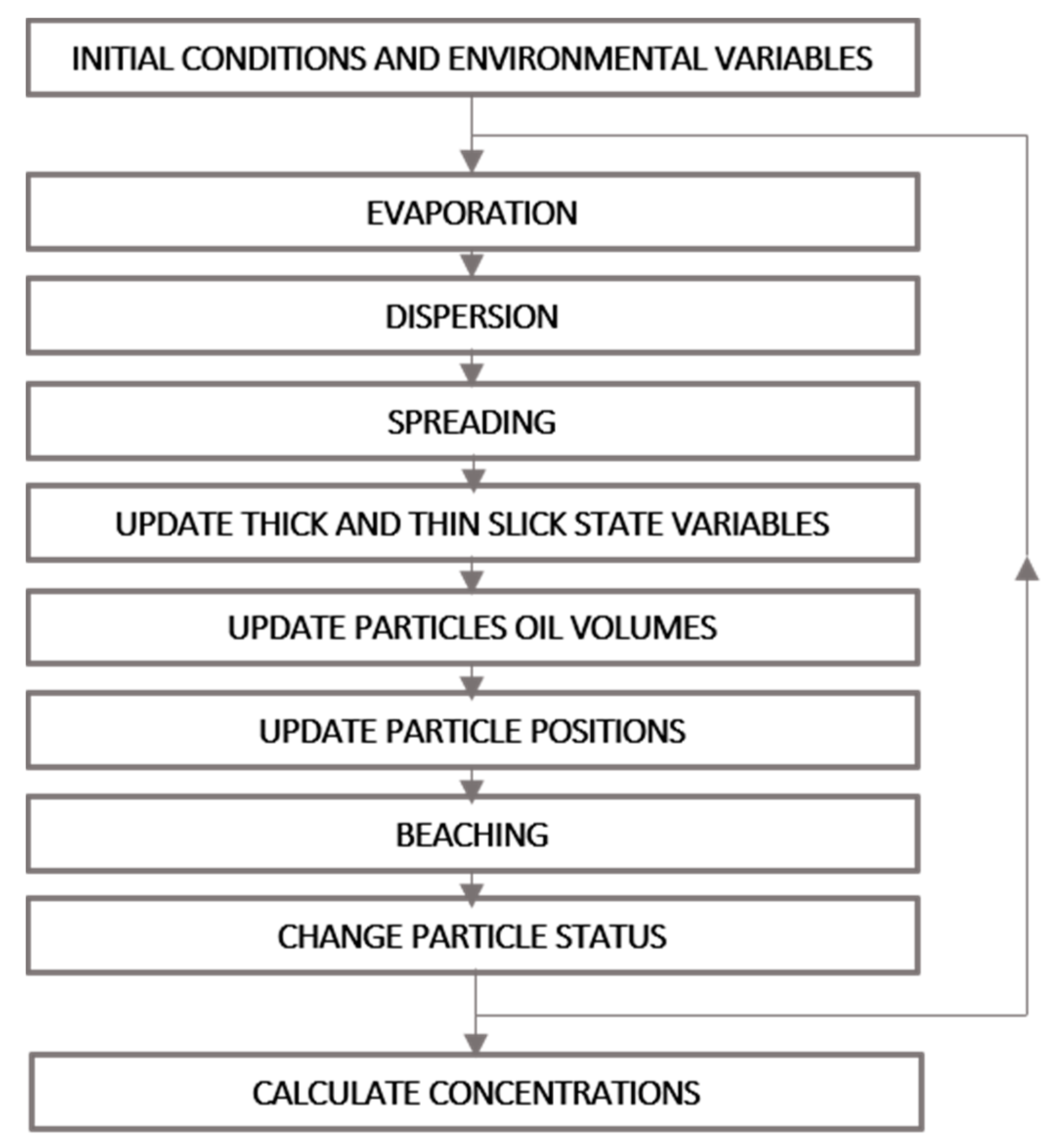
2.3. Oil Spill Model
3. Results and Discussion
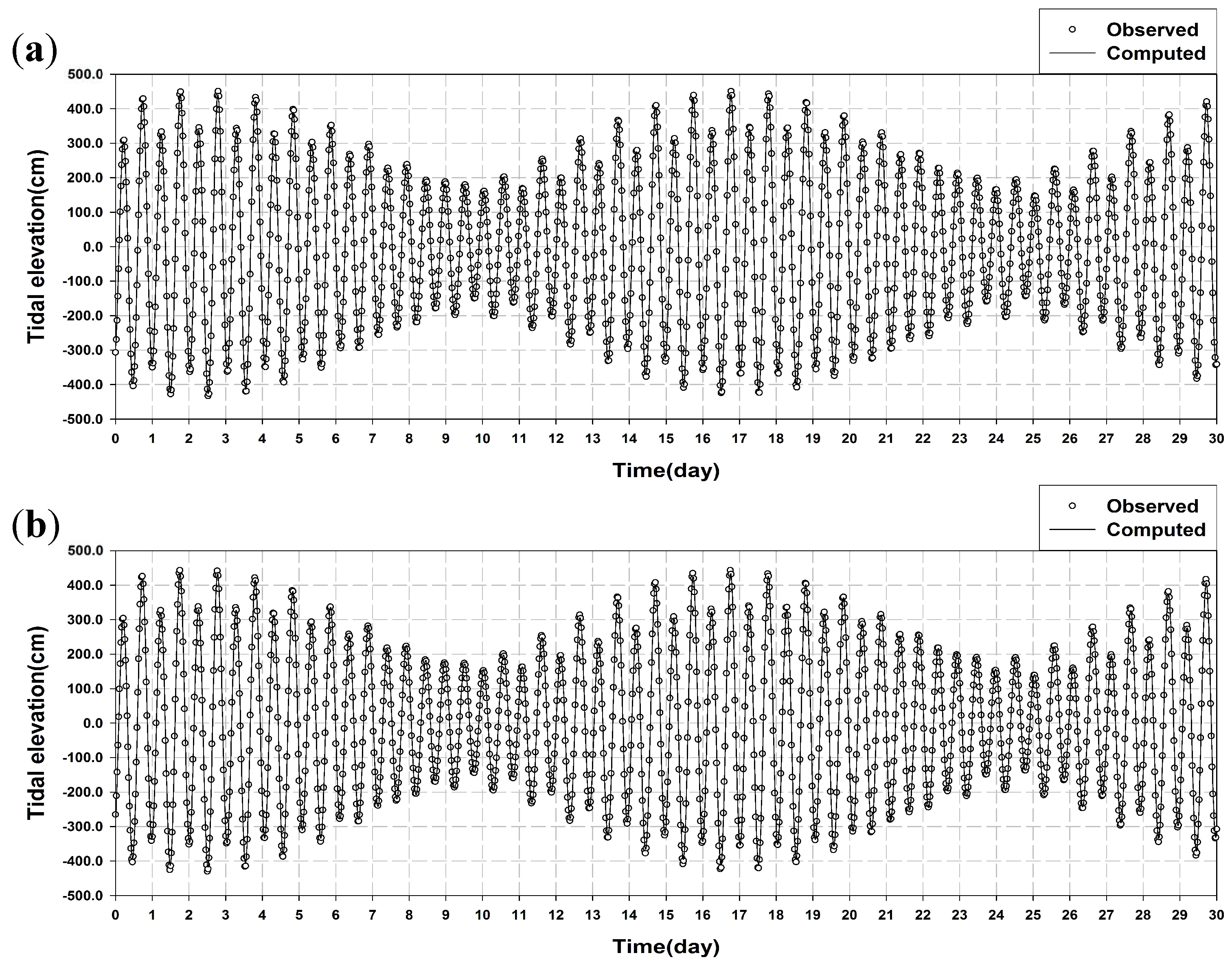
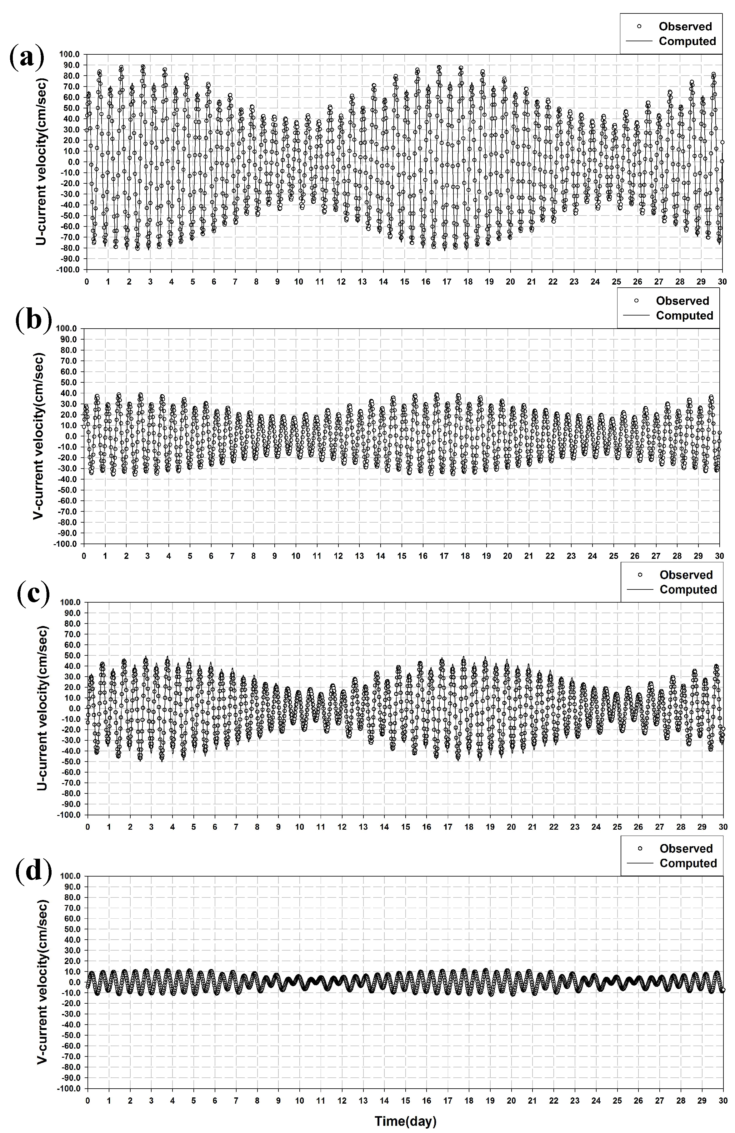
3.1. Model Verification
3.1.1. Tidal Elevation and Current
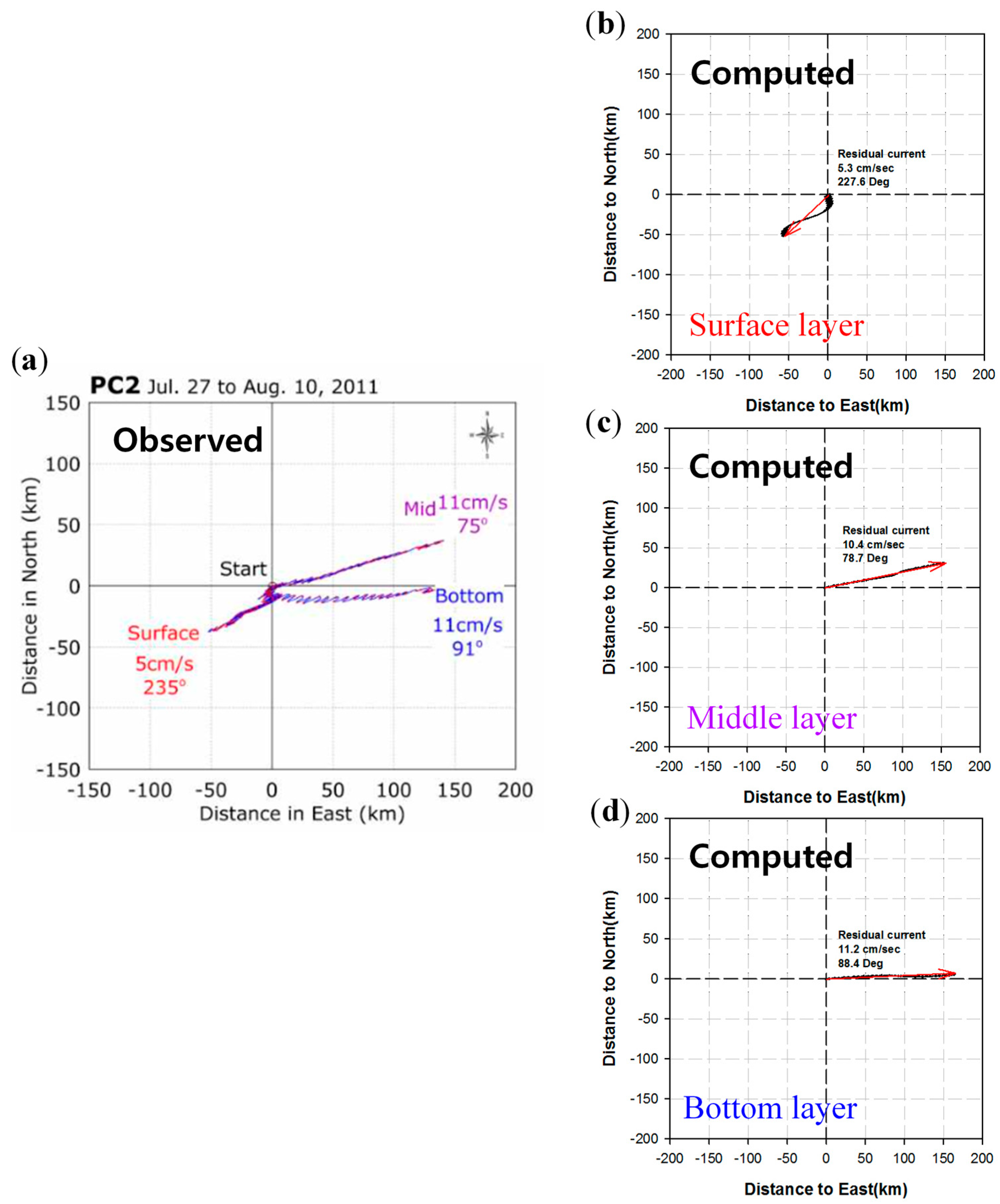
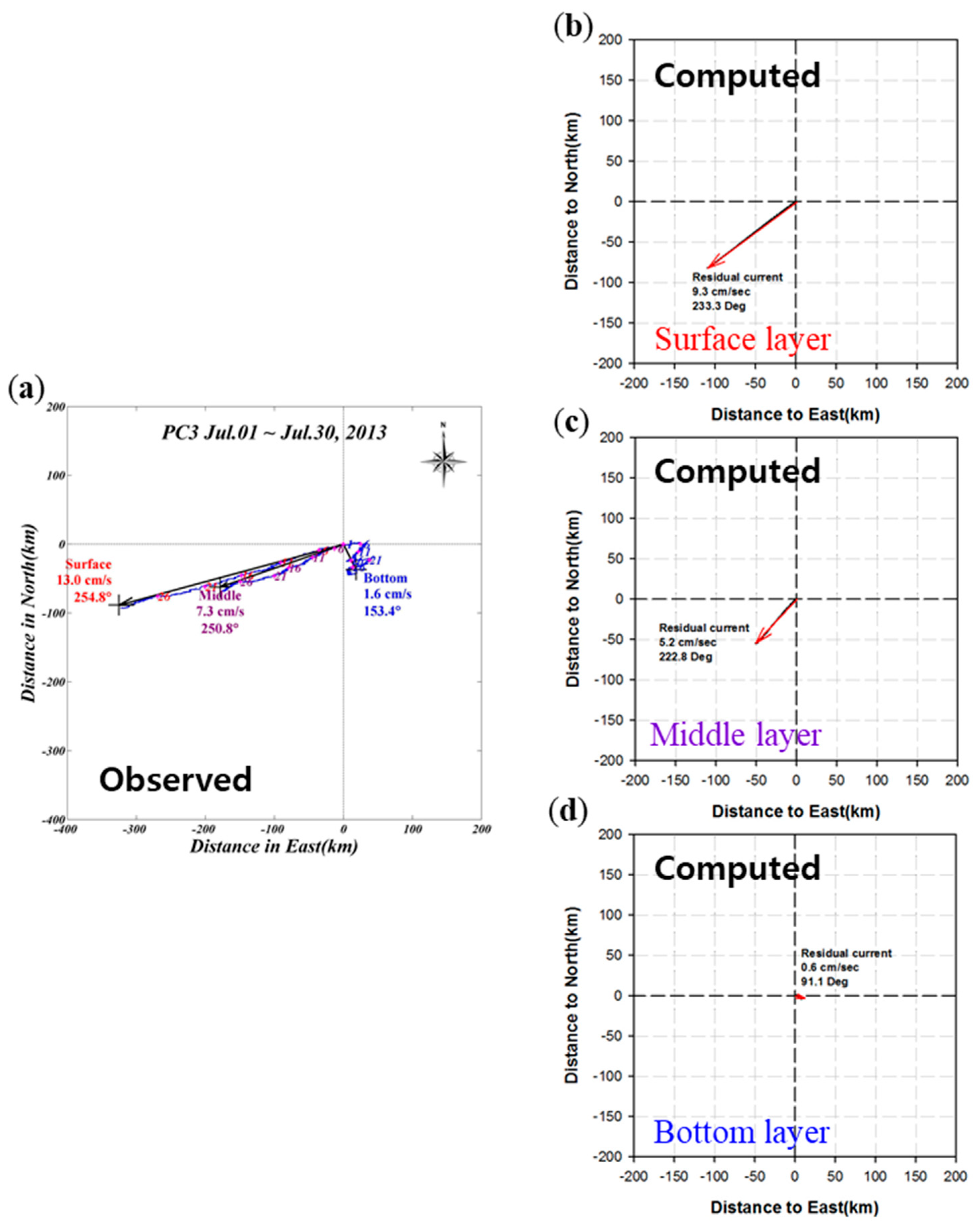
3.1.2. Residual Current
3.2. Tidal Currents Variation Considering Permeable Revetments
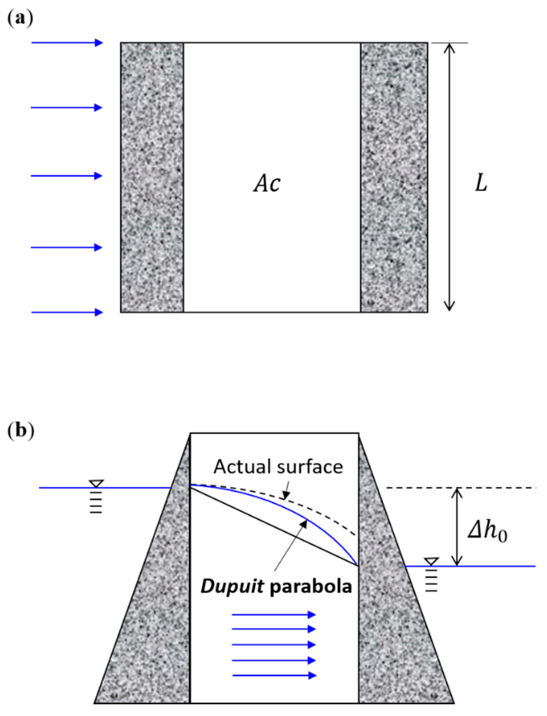
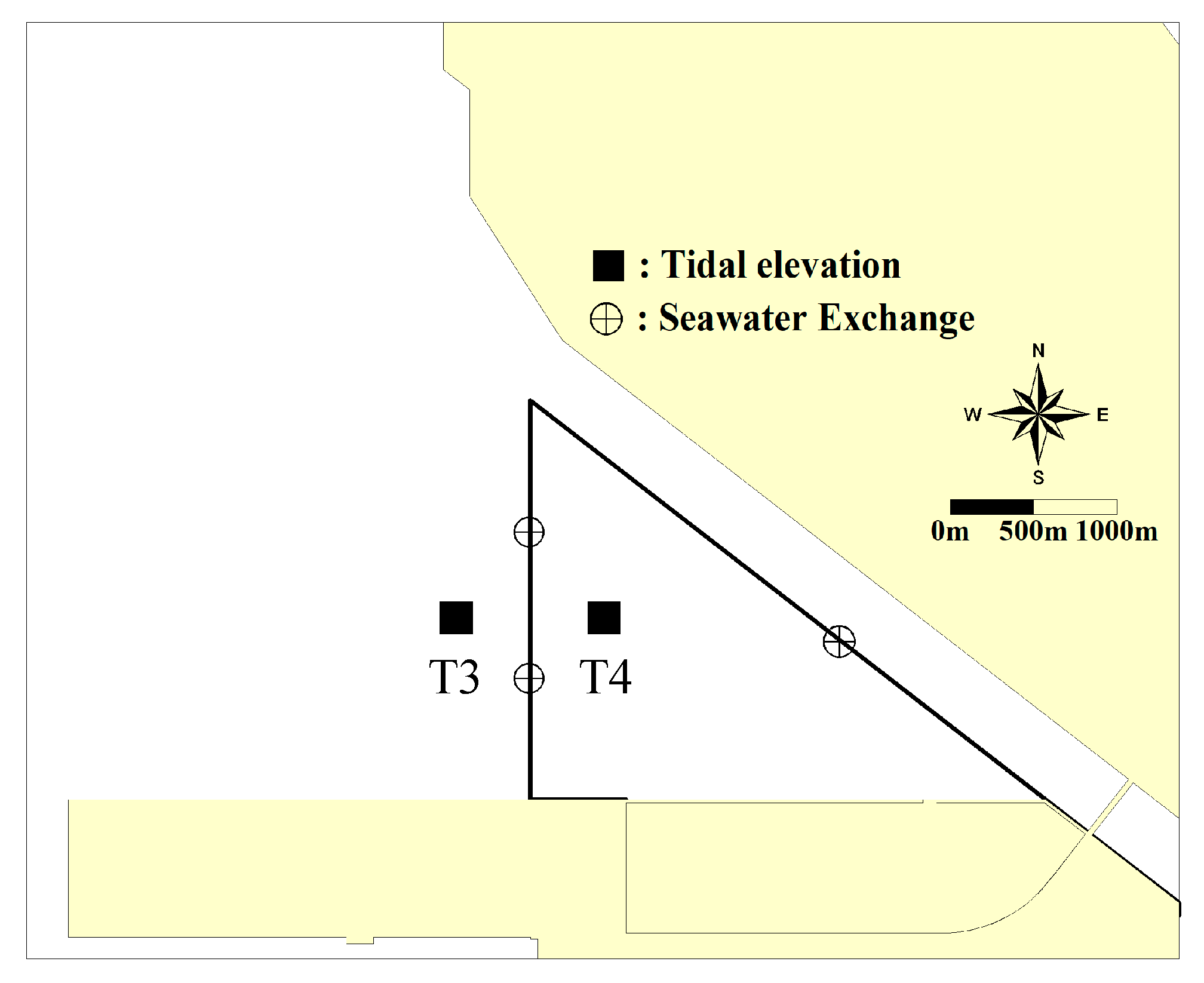
3.2.1. Water Circulation through Permeable Revetments
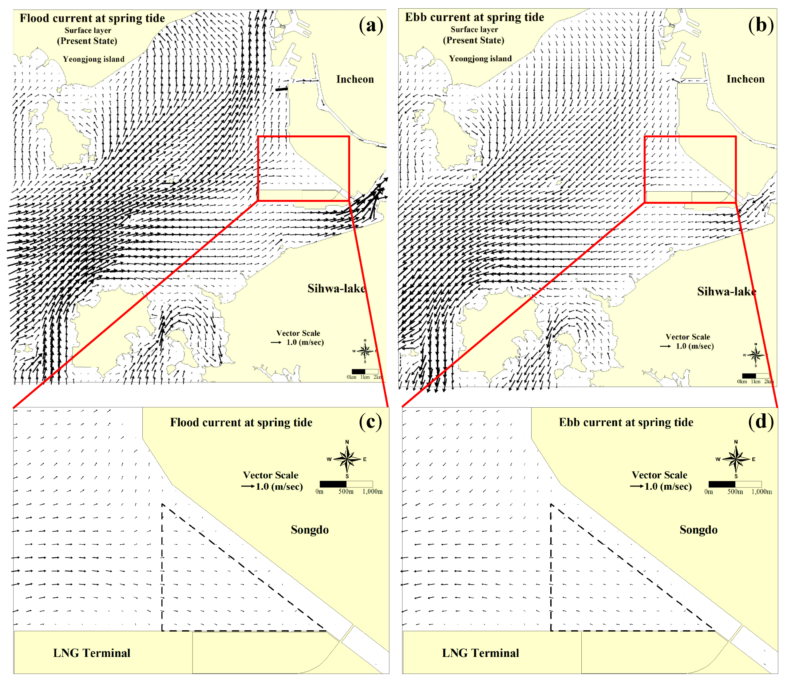
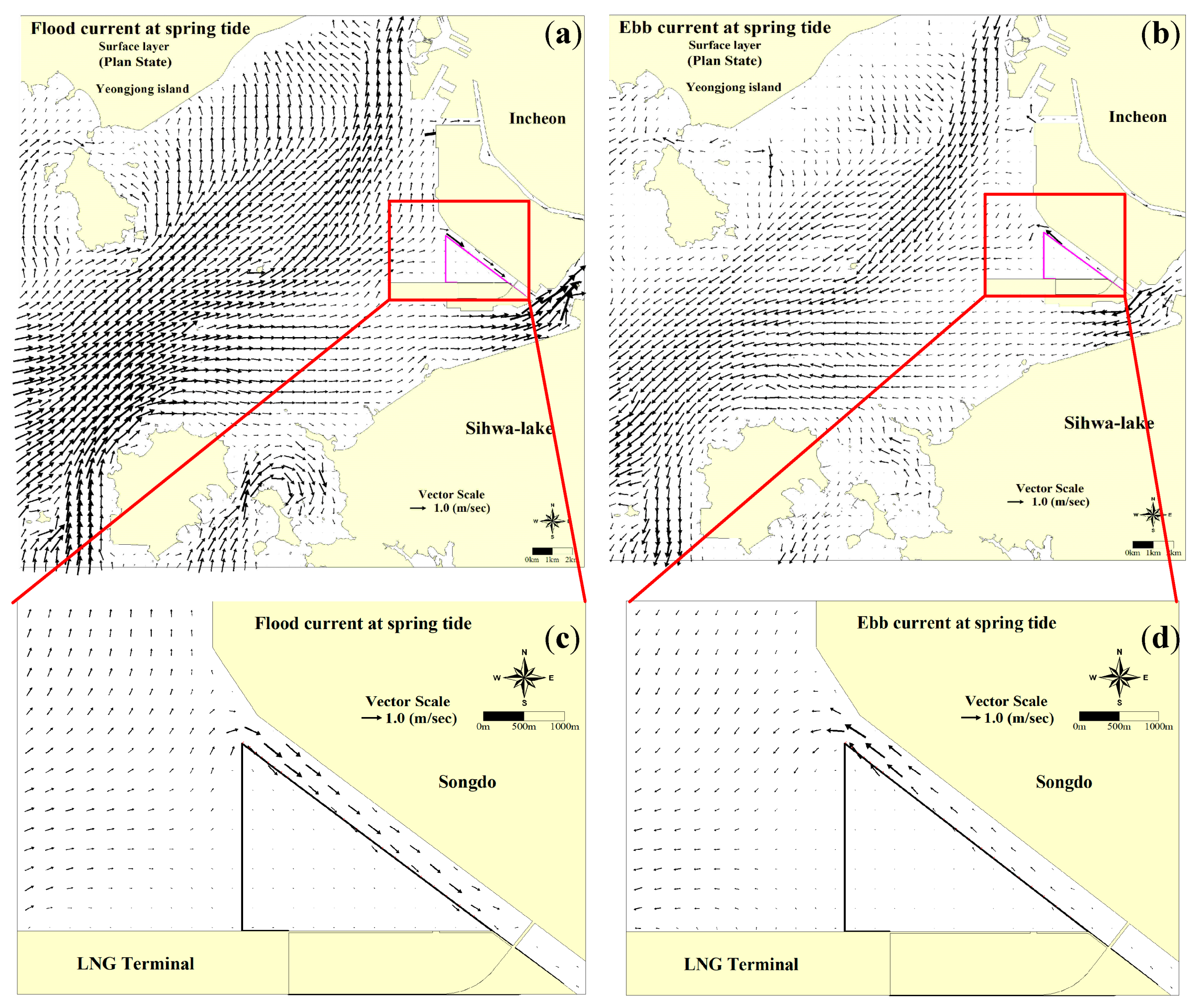
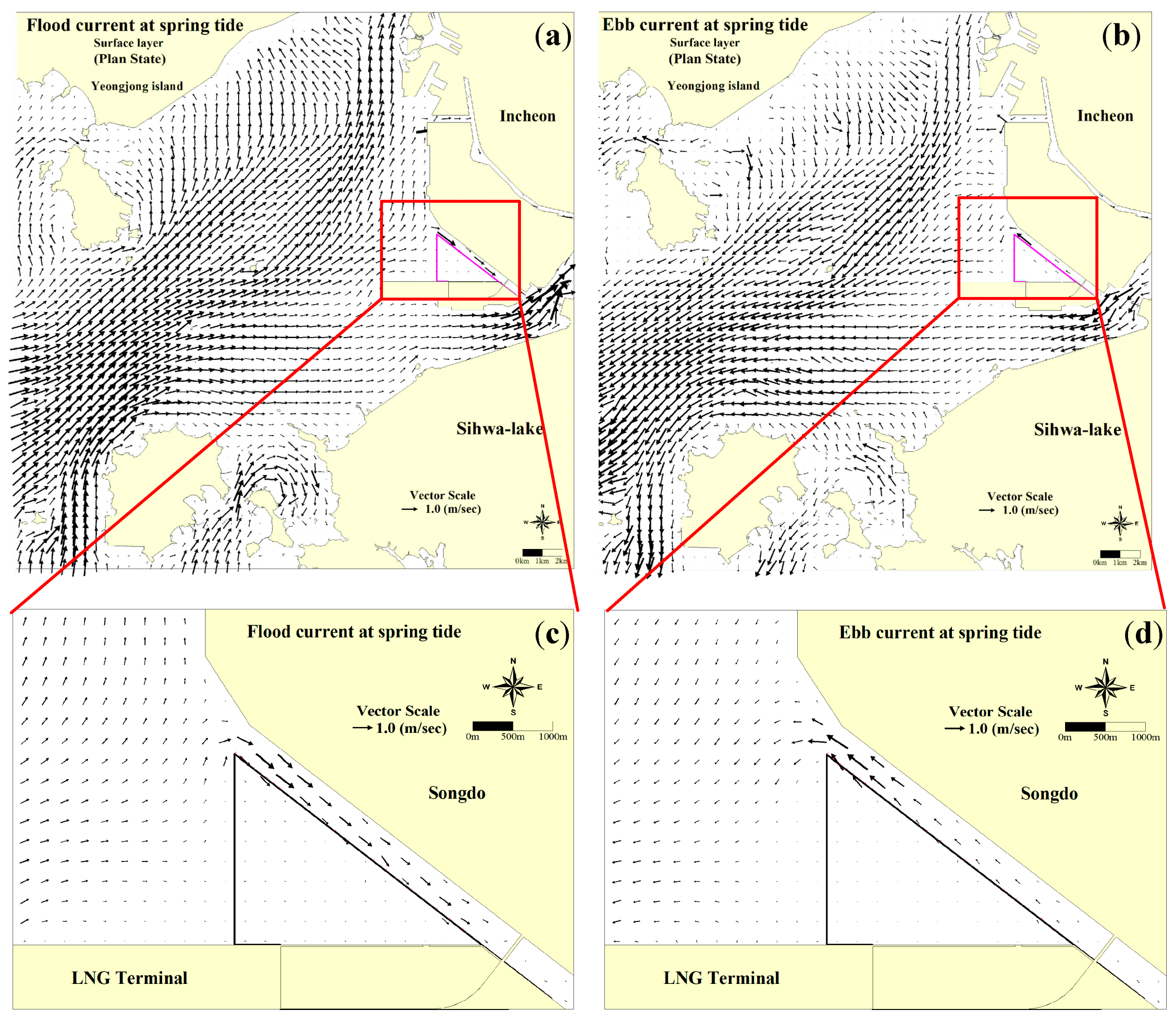
3.2.2. Tidal Current Velocity Fields
3.3. Oil Spill Dispersion
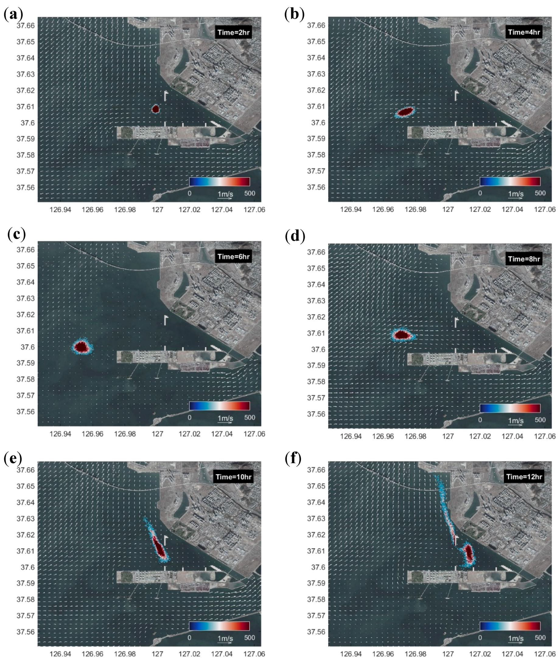
3.3.1. Scenario 1
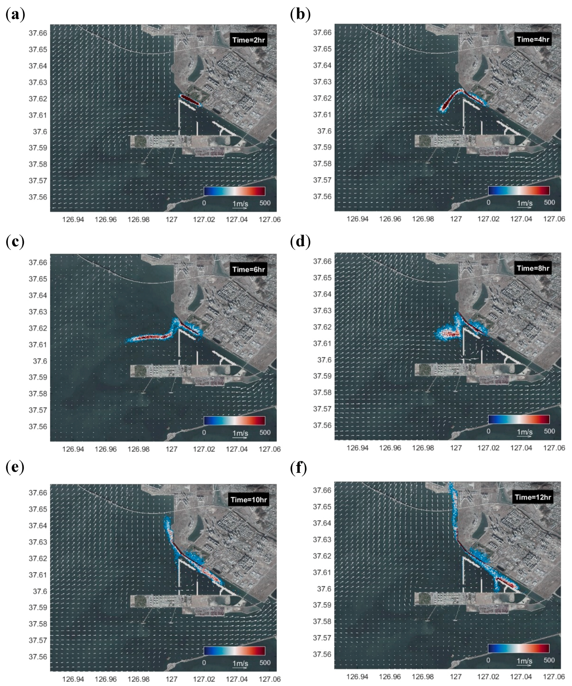
3.3.2. Scenario 2
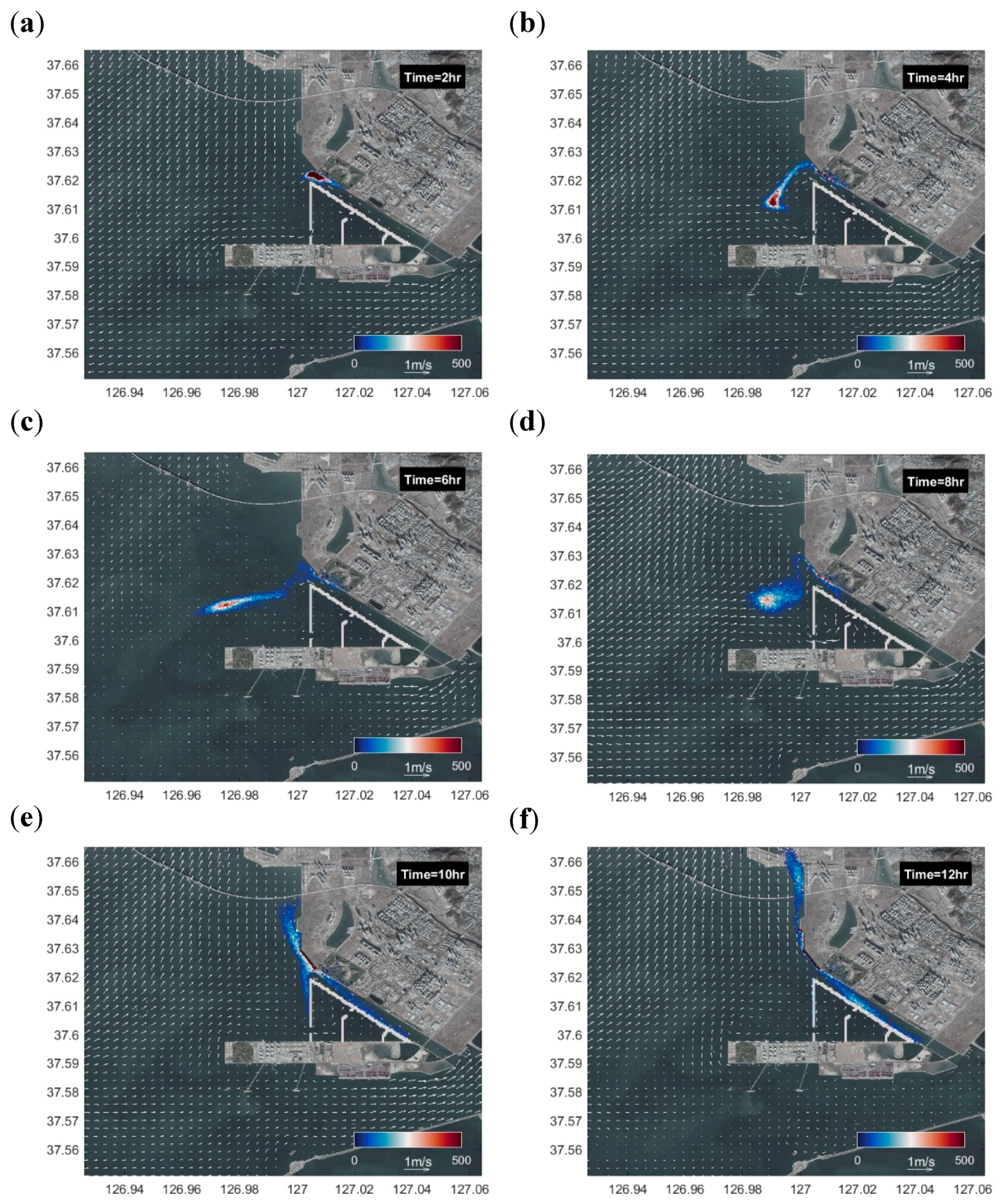
3.3.3. Scenario 3
4. Conclusions
Author Contributions
Funding
Institutional Review Board Statement
Informed Consent Statement
Data Availability Statement
Acknowledgments
Conflicts of Interest
References
- Xie, C.; Deng, J.; Zhuang, Y.; Sun, H. Estimating oil pollution risk in environmentally sensitive areas of petrochemical terminals based on a stochastic numerical simulation. Mar. Pollut. Bull. 2017, 123, 241–252. [Google Scholar] [CrossRef]
- Ribotti, A.; Antognarelli, F.; Cucco, A.; Falcieri, M.F.; Fazioli, L.; Ferrarin, C.; Olita, A.; Oliva, G.; Pes, A.; Quattrocchi, G. An Operational Marine Oil Spill Forecasting Tool for the Management of Emergencies in the Italian Seas. J. Mar. Sci. Eng. 2019, 7, 1. [Google Scholar] [CrossRef]
- Lee, K.-H.; Kim, T.-G.; Cho, Y.-H. Influence of Tidal Current, Wind and Wave in Hebei Spirit Oil Spill Modeling. J. Mar. Sci. Eng. 2020, 8, 69. [Google Scholar] [CrossRef]
- Beegle-Krause, C.J. GNOME:NOAA’s next-generation spill trajectory model. In Proceedings of the OCEANS’99 MTS/IEEE, Riding the Crest into the 21st Century, Seattle, WA, USA, 13–16 September 1999; pp. 1262–1266. [Google Scholar]
- Duran, R.; Romeo, L.; Whiting, J.; Vielma, J.; Rose, K.; Bunn, A.; Bauer, J. Simulation of the 2003 Foss Barge-Point Wells Oil Spill: A Comparison between BLOSOM and GNOME Oil Spill Models. J. Mar. Sci. Eng. 2018, 6, 104. [Google Scholar] [CrossRef]
- Castanedo, S.; Medina, R.; Losada, I.J.; Vidal, C.; Mendez, F.J.; Osorio, A.; Juanes, J.A.; Puente, A. The Prestige oil spillin Cantabria Bay of Biscay. Part I: Operational forecasting systemfor quick response, risk assessment, and protection of natural resources. J. Coast. Res. 2006, 22, 1474–1489. [Google Scholar] [CrossRef]
- Reed, M.; Gundlach, E.; Kana, T. A coastal zone oil spill model: Development and sensitivity studies. Oil Chem. Pollut. 1989, 5, 411–449. [Google Scholar] [CrossRef]
- Reed, M.; Aamo, O.M.; Daling, P.S. Quantitative analysis of alternate oil spill response strategies using OSCAR. Spill Sci. Technol. Bull. 1995, 2, 67–74. [Google Scholar] [CrossRef]
- Spaulding, M.; Kolluru, V.; Anderson, E.; Howlett, E. Application of three-dimensional oil spill model (WOSM/OILMAP) to hindcast the Braer spill. Spill Sci. Technol. Bull. 1994, 1, 23–35. [Google Scholar] [CrossRef]
- Al-Rabeh, A.H.; Lardner, R.W.; Gunay, N. Gulfspill Version 2.0: A software package for oil spills in the Arabian Gulf. Environ. Modell. Softw. 2000, 15, 425–442. [Google Scholar] [CrossRef]
- Lehr, W.; Jones, R.; Evans, M.; Simecek-Beatty, D.; Overstreet, R. Revisions of the ADIOS oil spill model. Environ. Model. Softw. 2022, 17, 189–197. [Google Scholar] [CrossRef]
- Daniel, P.; Marty, F.; Josse, P.; Skandrani, C.; Benshila, R. Improvement of Drift Calculation in Mothy Operational Oil Spill Prediction System. Int. Oil Spill Conf. Proc. 2003, 1, 1067–1072. [Google Scholar] [CrossRef]
- Carracedo, P.; Torres-López, S.; Barreiro, M.; Montero, P.; Balseiro, C.; Penabad, E.; Leitao, P.; Pérez-Muñuzuri, V. Improvement of pollutant drift forecast system applied to the Prestige oil spills in Galicia Coast (NW of Spain): Development of an operational system. Mar. Pollut. Bull. 2006, 53, 350–360. [Google Scholar] [CrossRef] [PubMed]
- Pollani, A.; Triantafyllou, G.; Petihakis, G.; Nittis, K.; Dounas, C.; Christoforos, K. The Poseidon operational tool for the prediction of floating pollutant transport. Mar. Pollut. Bull. 2001, 43, 270–278. [Google Scholar]
- Hackett, B.; Breivik, Ø.; Wettre, C. Forecasting the Drift of Objects and Substances in the Ocean. In Ocean Weather Forecasting; Springer: Dordrecht, The Netherlands, 2006; pp. 507–523. [Google Scholar] [CrossRef]
- Socolofsky, S.A.; Adams, E.E.; Boufadel, M.C.; Aman, Z.M.; Johansen, Ø.; Konkel, W.J.; Lindo, D.; Madsen, M.N.; North, E.W.; Paris, C.B. Intercomparison of Oil Spill Prediction Models for Accidental Blowout Scenarios with and without Subsea Chemical Dispersant Injection. Mar. Pollut. Bull. 2015, 96, 110–126. [Google Scholar] [CrossRef] [PubMed]
- De Dominicis, M.; Pinardi, N.; Zodiatis, G.; Lardner, R. MEDSLIK-II, a Lagrangian marine surface oil spill model for short-term forecasting—Part 1: Theory. Geosci. Model. Dev. 2013, 6, 1851–1869. [Google Scholar] [CrossRef]
- De Dominicis, M.; Pinardi, N.; Zodiatis, G.; Archetti, R. MEDSLIK-II, a Lagrangian marine surface oil spill model for short-term forecasting—Part 2: Numerical simulations and validations. Geosci. Model. Dev. 2013, 6, 1871–1888. [Google Scholar] [CrossRef]
- Coppini, G.; De Dominicis, M.; Zodiatis, G.; Lardner, R.; Pinardi, N.; Santoleri, R.; Colella, S.; Bignami, F.; Hayes, D.R.; Soloviev, D. Hindcast of oil-spill pollution during the Lebanon crisis in the Eastern Mediterranean, July–August 2006. Mar. Pollut. Bullet. 2011, 62, 140–153. [Google Scholar] [CrossRef]
- Neves, A.; Pinardi, N.; Martins, F.; Janeiro, J.; Samaras, A.; Zodiatis, G.; De Dominicis, M. Towards a common oil spill risk assessment framework adapting ISO 31000 and addressing uncertainties. J. Env. Manag. 2015, 159, 158–168. [Google Scholar] [CrossRef]
- Daewoo E&C. Design Report on the LNG Terminal Construction of the Incheon New Port; 2019; Unpublished Internal Report in Korean. [Google Scholar]
- Hamrick, J.M. A Three-Dimensional Environmental Fluid Dynamics Computer Code: Theoretical and computational aspects. In Special Report in Applied Marine Science and Ocean Engineering; Virginia Institute of Marine Science; College of William & Mary: Williamsburg, VA, USA, 1992; No. 317. [Google Scholar]
- Yang, Z.; Hamrick, J.M. Variational inverse parameter estimation in a cohesive sediment transport model: An adjoint approach. J. Geophys. Res. 2003, 108, 3055. [Google Scholar] [CrossRef]
- Mellor, G.L.; Yamada, T. Development of a turbulence closure model for geophysical fluid problems. Rev. Geophys. 1982, 20, 851–875. [Google Scholar] [CrossRef]
- Galperin, B.; Kantha, L.H.; Hassid, S.; Rosati, A. A Quasi-equilibrium Turbulent Energy Model for Geophysical Flows. J. Atmos. Sci. 1988, 45, 55–62. [Google Scholar] [CrossRef]
- Mackay, D.; Paterson, S.; Trudel, B. A mathematical model of oil spill behavior. Report to Research and Development Division, Environment Emergency Branch, Environmental Impact Control Directorate, Environmental Protection Service; Environment Canada: Ottawa, ON, Canada, 1980. [Google Scholar]
- Shaw, W.J.; Trowbridge, J.H. The Direct Estimation of Near-Bottom Turbulent Fluxes in the Presence of Energetic Wave Motions. J. Atmos. Oceanic Technol. 2001, 18, 1540–1557. [Google Scholar] [CrossRef]
- Imasato, N. What is Tide-Induced Residual Current? J. Phys. Oceanogr. 1983, 13, 1307–1317. [Google Scholar] [CrossRef]
- Wang, H.F.; Anderson, M.P. Introduction to Groundwater Modeling. In W.H. Freeman and Company; Academic Press: Cambridge, MA, USA, 1982. [Google Scholar]
- Samaras, A.G.; De Dominicis, M.; Archetti, R.; Lamberti, A.; Pinardi, N. Towards improving the representation of beaching in oil spill models: A case study. Mar. Pollut. Bull. 2014, 88, 91–101. [Google Scholar] [CrossRef] [PubMed]
- Etkin, D.S.; French-McCay, D.; Michel, J. Review of the State-of-the-Art on Modelling Interactions between Spilled Oil and Shorelines for the Development of Algorithms for Oil Spill Risk Analysis Modelling; Cortlandt Manor: NewYork, NY, USA, 2007; p. 157. [Google Scholar]
- Etkin, D. Worldwide Analysis of Marine oil Spill Cleanup Cost Factors (online). 2000. Available online: http://citeseerx.ist.psu.edu/viewdoc/download?doi=10.1.1.579.903&rep=rep1&type=pdf (accessed on 30 March 2021).
- Kim, Y.; Son, S.; Jung, T.; Gallien, T. An analytical and numerical study of a vertically discretized multi-paddle wavemaker for generating free surface and internal waves. Coast. Eng. 2021, 165, 103840. [Google Scholar] [CrossRef]
- Jung, T.; Son, S. Active tsunami generation by tectonic seafloor deformations of arbitrary geometry considering rupture kinematics. Wave Motion 2021, 100, 102683. [Google Scholar] [CrossRef]


| Scenario | Vessel Horsepower (HP) | Tanker Capacity (L) | Oil Spillage Volume (L) | Initial Spill Location |
|---|---|---|---|---|
| 1 | 3200 | 42,000 | 29,400 | Western revetment |
| 2 | 2600 | 33,000 | 23,100 | Eastern revetment |
| 3 | 1000 | 15,000 | 10,500 | Eastern revetment |
| Tidal Elevation | Amplitude (cm) | Phase (°) | Approximation Relative Error (%) | |||
|---|---|---|---|---|---|---|
| Gauge Station | Constituents | Observed | Computed | Observed | Computed | |
| T1 | M2 | 286.2 | 279.3 | 141.4 | 138.5 | 2.0 |
| S2 | 112.7 | 110.6 | 201.6 | 197.7 | ||
| K1 | 39.4 | 39.1 | 306.8 | 305.8 | ||
| O1 | 25.2 | 25.4 | 265.7 | 266.6 | ||
| T2 | M2 | 278.5 | 127.5 | 274.0 | 134.0 | 2.5 |
| S2 | 112.6 | 184.3 | 108.6 | 192.0 | ||
| K1 | 38.8 | 301.7 | 39.2 | 302.8 | ||
| O1 | 28.5 | 262.1 | 25.2 | 263.5 | ||
| Horizontal Velocity (U) | Amplitude, A (cm/s) | Phase, θ (°) | Approximation Relative Error, Eapp (%) | |||
|---|---|---|---|---|---|---|
| Gauge Station | Constituents | Observed | Computed | Observed | Computed | |
| PC1 | M2 | 59.2 | 57.9 | 45.8 | 46.6 | −0.3 |
| S2 | 20.3 | 23.5 | 105.7 | 106.2 | ||
| K1 | 6.6 | 5.0 | 238.1 | 217.1 | ||
| O1 | 3.1 | 3.1 | 188.5 | 183.9 | ||
| PC2 | M2 | 34.1 | 33.6 | 38.9 | 50.0 | −8.3 |
| S2 | 9.9 | 17.5 | 281.4 | 307.7 | ||
| K1 | 4.1 | 3.2 | 217.8 | 217.8 | ||
| O1 | 3.8 | 1.9 | 232.6 | 182.0 | ||
| PC3 | M2 | 28.8 | 29.8 | 95.2 | 94.5 | −6.3 |
| S2 | 12.9 | 16.8 | 172.3 | 180.1 | ||
| K1 | 4.2 | 3.8 | 296.0 | 300.9 | ||
| O1 | 3.5 | 2.1 | 274.2 | 274.9 | ||
| Vertical Velocity (V) | Amplitude, A (cm/s) | Phase, θ (°) | Approximation Relative Error, Eapp (%) | |||
|---|---|---|---|---|---|---|
| Gauge Station | Constituents | Observed | Computed | Observed | Computed | |
| PC1 | M2 | 26.3 | 24.5 | 57.8 | 42.8 | 3.1 |
| S2 | 8.3 | 9.7 | 110.1 | 103.3 | ||
| K1 | 2.9 | 2.2 | 251.2 | 217.1 | ||
| O1 | 1.7 | 1.6 | 204.0 | 170.7 | ||
| PC2 | M2 | 34.3 | 33.2 | 45.5 | 50.2 | 9.7 |
| S2 | 15.7 | 13.1 | 30.9 | 39.5 | ||
| K1 | 4.5 | 2.4 | 219.7 | 217.8 | ||
| O1 | 1.0 | 1.4 | 15.8 | 15.0 | ||
| PC3 | M2 | 7.3 | 7.0 | 111.6 | 121.4 | 3.6 |
| S2 | 3.5 | 4.0 | 193.1 | 188.7 | ||
| K1 | 1.7 | 1.5 | 296.0 | 300.0 | ||
| O1 | 1.3 | 0.8 | 30.9 | 33.2 | ||
| Condition | Tidal Elevation at High Tide (m) | Δh0 (m) | |
|---|---|---|---|
| T3 | T4 | ||
| Without passage | 9.19 | 7.73 | 1.46 |
| With passage | 9.19 | 8.37 | 0.82 |
Publisher’s Note: MDPI stays neutral with regard to jurisdictional claims in published maps and institutional affiliations. |
© 2021 by the authors. Licensee MDPI, Basel, Switzerland. This article is an open access article distributed under the terms and conditions of the Creative Commons Attribution (CC BY) license (https://creativecommons.org/licenses/by/4.0/).
Share and Cite
Na, B.; Son, S.; Choi, J.-C. Modeling of Accidental Oil Spills at Different Phases of LNG Terminal Construction. J. Mar. Sci. Eng. 2021, 9, 392. https://doi.org/10.3390/jmse9040392
Na B, Son S, Choi J-C. Modeling of Accidental Oil Spills at Different Phases of LNG Terminal Construction. Journal of Marine Science and Engineering. 2021; 9(4):392. https://doi.org/10.3390/jmse9040392
Chicago/Turabian StyleNa, Byoungjoon, Sangyoung Son, and Jae-Cheon Choi. 2021. "Modeling of Accidental Oil Spills at Different Phases of LNG Terminal Construction" Journal of Marine Science and Engineering 9, no. 4: 392. https://doi.org/10.3390/jmse9040392
APA StyleNa, B., Son, S., & Choi, J.-C. (2021). Modeling of Accidental Oil Spills at Different Phases of LNG Terminal Construction. Journal of Marine Science and Engineering, 9(4), 392. https://doi.org/10.3390/jmse9040392