Article

Increasing Trends in Air and Sea Surface Temperature in the Central Adriatic Sea (Croatia)

1
Faculty of Civil Engineering, Architecture and Geodesy, University of Split, Matice Hrvatske 15, 21000 Split, Croatia
2
Faculty of Croatian Studies, University of Zagreb, Borongajska Cesta 83d, 10000 Zagreb, Croatia
3
Department of Hydrogeology and Engineering Geology, Croatian Geological Survey, Sachsova 2, 10000 Zagreb, Croatia
*
Author to whom correspondence should be addressed.
J. Mar. Sci. Eng. 2021, 9(4), 358; https://doi.org/10.3390/jmse9040358
Submission received: 30 January 2021 / Revised: 10 March 2021 / Accepted: 23 March 2021 / Published: 26 March 2021
(This article belongs to the Special Issue Sea Surface Temperature: From Observation to Applications)

Abstract

:
The Adriatic Sea and its coastal region have experienced significant environmental changes in recent decades, aggravated by climate change. The most prominent effects of climate change (namely, an increase in sea surface and air temperature together with changes in the precipitation regime) could have an adverse effect on social and environmental processes. In this study, we analyzed the time series of sea surface temperature and air temperature measured at three meteorological stations in the Croatian part of the Adriatic Sea. To assess the trends and variations in the time series of sea surface and air temperature, different statistical methods were employed, i.e., linear and quadratic regressions, Mann–Kendall test, Rescaled Adjusted Partial Sums method, and autocorrelation. The results evidenced increasing trends in the mean annual sea surface temperature and air temperature; furthermore, sudden variations in values were observed in 1998 and 1992, respectively. Increasing trends in the mean monthly sea surface temperature and air temperature occurred in the warmer parts of the year (from March to August). The results of this study could provide a foundation for stakeholders, decision–makers, and other scientists for developing effective measures to mitigate the negative effects of climate change in the scattered environment of the Adriatic islands and coastal region.

1. Introduction

The Adriatic Sea is the northernmost part of the Mediterranean Sea and represents a vast bay that is indented far into the European mainland. The surface of the Adriatic Sea is 138,595 km2, which constitutes 4.6% of the total surface of the Mediterranean Sea. The Adriatic Sea stretches in NW–SE direction for 870 km, with an average width of approximately 200 km. It is connected to the Mediterranean Sea by the 70 km–wide Strait of Otranto. The Adriatic Sea is heterogeneous in terms of physical, chemical, and biological properties [1]. Based on the average depth, the Adriatic is divided into (i) very shallow Northern Adriatic (<35 m), (ii) Central Adriatic Sea (~140 m), and (iii) Southern Adriatic with an average depth of >200 m and maximum depth up to 1228 m [2]. The majority of the islands in the Adriatic Sea are within the Croatian territory. The total length of the Croatian coast is 5835 km, i.e., the lengths of the island and mainland coast are 4058 km and 1777 km, respectively.
One of the key environmental questions is how climate change, particularly global warming, will affect the environmental and social processes in different regions of the planet. The investigation of the effects of climate change in the coastal environment is a particularly complex task because of the simultaneous influence of vast land and water masses, which react differently to climate change. Since climate change continues to intensify, both the Adriatic and the Mediterranean regions are considered hot spots of climate change. In particular, the Adriatic ecosystems suffer the combined effect of climate change in the Northern hemisphere and local climate variations [3]. Regional atmospheric oscillations, as a result of the air pressure variations in the Northern hemisphere, and the intensification of water inflow from the Eastern Mediterranean affected the Adriatic Sea temperature and salinity. Further local factors impacting the Adriatic marine ecosystems are: (i) increasing sea surface temperature, (ii) negative trends in the precipitation patterns, particularly in the winter season, and (iii) reduced inflow of fresh water and nutrients as a result of the decreasing inflow from the Po river [4]. This complex situation is fostered by the variable geometry and topography of the Adriatic region where each bay, island, or channel in the Adriatic Sea is site–specific in terms of oceanographic properties [5] and reactions to climate change [6,7]. The devastation of the environment, the increasing demand for fresh water for potable and irrigation purposes, and the changes in the already unfavorable water balances of the Mediterranean semi–arid climate could lead to adverse environmental and social consequences in the near future. Commonly, the karst environments are scarce in surface hydrography and groundwater is the main freshwater resource. Hence, the Mediterranean water resources are under significant stress due to over–abstraction, climate change, and the high possibility of seawater intrusions into karst aquifers in the coastal areas or the islands.
To understand the trends and the behavior of the air temperature on small islands and in the coastal areas, it is necessary to understand the interaction between the sea surface temperature and the air temperature. Vlahakis and Pollatou [8] emphasized that the sea surface temperature is the key factor in the assessment of the climate and climate–related processes on all scales, especially on the islands and in the coastal areas. Sea surface temperature has a direct influence on global energy transfer, atmospheric processes, precipitation, evapotranspiration, moisture in air and soil, wind development, hydrological cycle, and other ecological or social processes [9]. However, sea surface temperature is not considered a standard meteorological parameter even though its effect on the atmosphere is immense. Furthermore, the time series of the sea surface temperature are considerably shorter when compared to the air temperature. The sea has a higher thermal capacity than the land, resulting in slower heating and cooling. During winter and summer, the sea acts as a buffer that moderates the air temperature, resulting in a lower range of the sea surface temperature than the range of air temperature over land [10]. The flow of the seawater and other turbulent processes cause the deeper layers of the sea to mix with the surficial ones, influencing the air temperature. The air temperature reacts differently to changes in the sea surface temperature, and this is particularly pronounced on the small islands and in the coastal areas. Therefore, it is necessary to analyze each location based on a detailed and reliable time series of measured data.
Time series of the sea surface temperature and the air temperature measured at three meteorological stations located on Central Adriatic islands (Hvar and Vis) and on the mainland (Split) were analyzed in this study. Firstly, we will describe the study area and the available dataset. The dataset will be analyzed using different statistical approaches and the obtained results will be used to assess the occurrence of trends within the time series of the sea surface temperature and the air temperature. These data will provide a foundation for stakeholders, decision–makers, and other scientists for developing effective measures to mitigate the negative effects of climate change in the Adriatic region and beyond.

2. Study Area

The study area is located in the central part of the Adriatic Sea and consists of the two meteorological stations on the islands of Hvar and Vis, and the meteorological station in the city of Split on the mainland. The map of the study area showing the analyzed meteorological stations is in Figure 1.
The main characteristics of the analyzed stations used in this study are summarized in Table 1.
The meteorological station Split is located in the eastern part of Split, on the Marjan peninsula. Marjan is a forest park used for recreational purposes. The meteorological station is in the vicinity of the second tallest peak on Marjan (178 m a.s.l.). In 2011, the population of Split was 178,192. Despite rapid urbanization of the Split agglomeration, the meteorological station Split is not affected by urbanization due to its position within a protected forest area. The sea surface temperature (SST hereafter) is measured at the endpoint of the pier at the easternmost point of the Marjan peninsula.
The small island of Hvar belongs to the Middle–Dalmatian island group. With a surface area of 297.32 km2 and a coastline of 270 km, Hvar is the fourth biggest island in the Croatian part of the Adriatic Sea [11]. In 2011, the city of Hvar had a population of 4251. The meteorological station Hvar is situated in a small forest grove, away from the urbanized city center. The SST is measured at the endpoint of a small pier 100 m from the meteorological station.
Vis is a small remote island in the Adriatic Sea. Its distance from the mainland is 43 km and the island is exposed to very strong winds. With a surface area of 89.72 km2 and coastline of 85 km, Vis is the ninth biggest island in the Croatian part of the Adriatic Sea [11]. The meteorological station is located in the city of Komiža, on the northern edge of the urbanized area. In 2011, Komiža had a population of 1526. The SST is measured at the endpoint of a pier in Komiža, 190 m from the meteorological station. Vis Island has favorable geological and hydrogeological conditions that have enabled the formation of high–quality karst aquifers from which the fresh water is abstracted. Hence, Vis Island and its groundwater resources are considered highly vulnerable to climate change [7].
According to Köppen–Geiger climate classification, the study area is characterized by the Csa climate type [12], sometimes called the “olive” climate. It is a semiarid variety of Mediterranean climate characterized by mild and humid winters, and dry and hot summers.

3. Materials and Methods

3.1. Data Collection

The SST and the air temperature data used in this study were provided by the Croatian Meteorological and Hydrological Service (DHMZ). The conventional method of measuring the SST is performed using a thermometer immersed in the sea at a depth of 30 cm, given that the sea is not shallower than 180 cm at the measuring point. The thermometer is immersed for three minutes, and after that, it is taken out and read quickly [13]. The SST is measured three times a day at 7, 14, and 21 h local time. The measurement of the SST is performed by personnel from the nearby meteorological station. Values of the mean monthly and the mean annual SST were analyzed in this study.
Furthermore, the time series of air temperature were measured at main meteorological stations. An interesting fact is that the meteorological station Hvar started to operate in 1858, followed by the Split station a year after, and Komiža in 1959. The World Meteorological Organization (WMO) recognized the quality of the station in Hvar and awarded it a Centennial Observing Station title. The air temperature is measured hourly at a standard height of 2 m above the ground. In this study, the mean monthly and the mean annual air temperature for the period 1960–2019 were analyzed. Despite several approaches (e.g., [14,15,16]), the method employed by the DHMZ [13], which is the most common in Europe, defines the mean daily air temperature as:
t   m e a n , d a i l y = t 7 + t 14 + 2 t 21 4 ,
where t7, t14, and t21 are the air temperature values measured at 7, 14, and 21 h (local time), respectively. The same procedure is applied for the SST.

3.2. Statistical Methods

Linear and quadratic regressions were performed on the time series of mean monthly and mean annual SST and air temperature from three stations analyzed in this study. The linear regression equation is given as:
T = (a × t) + b,
and the quadratic regression equation as:
T = (c × t2) + (d × t) + e,
where T is the mean monthly or mean annual SST or air temperature in year t, a and b are linear regression coefficients, and c, d, and e are quadratic regression coefficients. All five coefficients are calculated by the least–squares method. The coefficient a represents the slope of the regression line whose dimension is °C/year, and it is the indicator of the average intensity of the increasing or decreasing trends in the values of the analyzed time series. The correlation coefficients r2 and R2 were calculated for the linear and the quadratic regressions, respectively. Both coefficients show the strength and the direction of linear and quadratic correlation between variables x (time) and y (the mean monthly or the mean annual SST or air temperature).
To assess whether the time series have monotonic increasing or decreasing trends, the Mann–Kendall (M–K hereafter) non–parametric test was used [17]. The null hypothesis for this test is that there is no monotonic trend within the analyzed time series, while the alternate hypothesis is that the trend exists. As a criterion to accept the alternate hypothesis (i.e., the presence of an increasing or decreasing trend), p–values < 0.05 were used in this study.
Furthermore, the Rescaled Adjusted Partial Sums method (RAPS hereafter) was used to detect statistically significant peaks or declines in values (i.e., the trends variations) within the analyzed time series [18,19]. This method allows overcoming random and irregular fluctuations as well as rough errors in values within the time series, which may be hidden from the common plots of values of the time series. Based on the RAPS results, sub–periods with similar characteristics or a larger number of trends within the time series could be distinguished. The formula for the calculation of RAPS is:
R A P S k = t = 1 k Y t Y m S y ,  
where Yt is the value of the observed parameter at time t, Ym is the mean value of observed time series, Sy is the standard deviation of the observed time series, and k is the number of observations. The breakpoints between the sub–periods were established when the trend of RAPS results showed a significant variation.
The differences in statistical parameters of the two neighboring sub–periods defined by the RAPS were evaluated by the F–test and the t–test [20]. In particular, the F–test was used to assess the equality of variances between the two normally distributed populations (i.e., sub–periods). The t–test was used to determine whether there is a statistical difference between the mean values of the two sub–periods. In this study, both tests accept the null hypothesis for p–values < 0.05.
Furthermore, the autocorrelation of the time series was determined. Autocorrelation is a mathematical function representing the degree of similarity between the specific time series and a lagged version of the same time series over successive time intervals. Autocorrelation coefficient r ranges from −1 to 1 and it measures the strength of a relationship between the current value of the variable with its shifted value. In this study, the interval of the shifting variable was set to 1 year. For r < 0.2, the time series is not autocorrelated meaning that the behavior of the values does not depend on the previous values [21].

4. Results and Discussion

In this chapter, temporal changes in the mean annual and the mean monthly SST and air temperature were analyzed. The analyzed time series are not identical in duration, which will affect the reliable comparison of the results obtained at three analyzed stations to a minor extent. Despite the differences in the duration of the analyzed time series, contemporaneous time series were available for the last 29–year period (i.e., 1991–2019), when the most significant increases in the SST and the air temperature were observed. This fact will allow a more reliable conclusion about the recent and future behavior of the SST and the air temperature in the study area.

4.1. Analyses of the Mean Annual Sea Surface Temperature and Air Temperature

Table 2 shows a summary of the exploratory statistical analysis (minimum, average, maximum, and range) of the mean annual SST, the air temperature (TA), and their difference (ΔT = SST–T
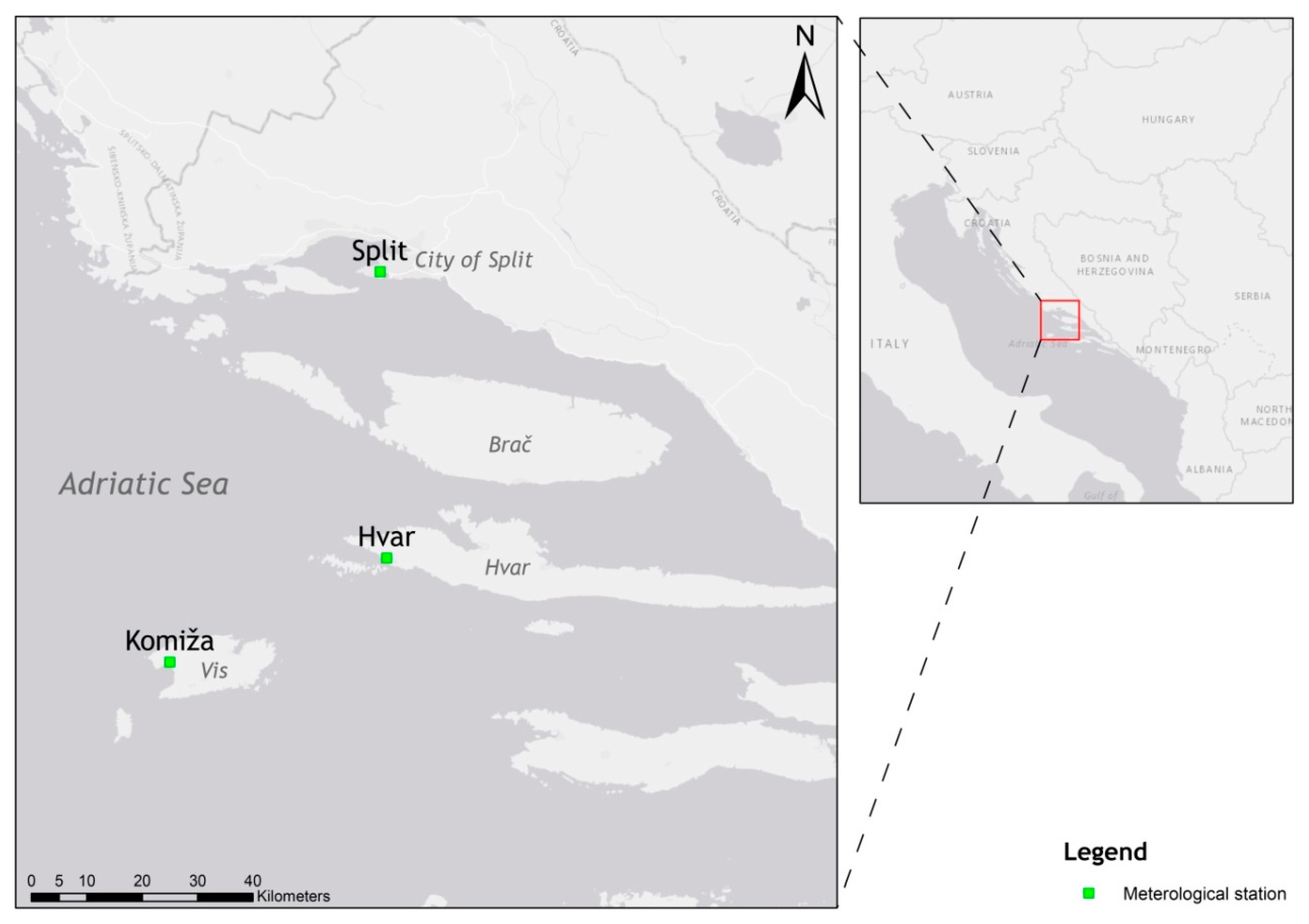
A) at the analyzed stations. The longest time series analyzed in this study were recorded in Split (from 1960 to 2019), followed by Hvar (from 1964 to 2019), and Komiža with the shortest time series (from 1991 to 2019).
The minimum, average, and maximum values of the mean annual SST measured in Split were 16.3 °C, 17.4 °C, and 18.7 °C, respectively. The values measured at Hvar were slightly higher being 17 °C, 18.1 °C, and 19.3 °C, respectively. Komiža had the highest values of SST, with the minimum, average, and maximum mean annual SST being 17.9 °C, 18.9 °C, and 19.5 °C, respectively. The range of the mean annual SST was 2.4 °C, 2.3 °C, and 1.6 °C in Split, Hvar, and Komiža, respectively. The lowest range of the mean annual SST in Komiža reflects its furthest position in the open sea among the analyzed stations.
The distribution of the air temperature (TA) values was similar to the SST in terms of Split having the lowest values and Komiža the highest. The minimum, average, and maximum values of the mean annual air temperature measured in Split were 15.1 °C, 16.4 °C, and 17.8 °C, respectively; slightly higher values were measured in Hvar as 15.5 °C, 16.7 °C, and 18.2 °C, respectively. In Komiža, the minimum, average, and maximum values of the mean annual air temperature were 16.2 °C, 17.2 °C, and 18 °C. Hvar and Split had an identical range of the mean annual air temperature, 2.7 °C, while the range in Komiža was 1.8 °C.
The ΔT values (SST-TA) showed the same distribution as the SST and the TA. The ΔT of the minimum values were 1.2 °C, 1.5 °C, and 1.7 °C, in Split, Hvar, and Komiža, respectively. The ΔT average values were 1.1 °C, 1.4 °C, and 1.7 °C, while the ΔT maximum values were 0.9 °C, 1.1 °C, and 1.5 °C at the same stations, respectively. The positive values of ΔT indicated that the mean annual SST was always higher than the mean annual air temperature. It should be noted that ΔT of the minimum values were higher than the ΔT of the maximum values due to the smaller amplitude of the SST than the air temperature.
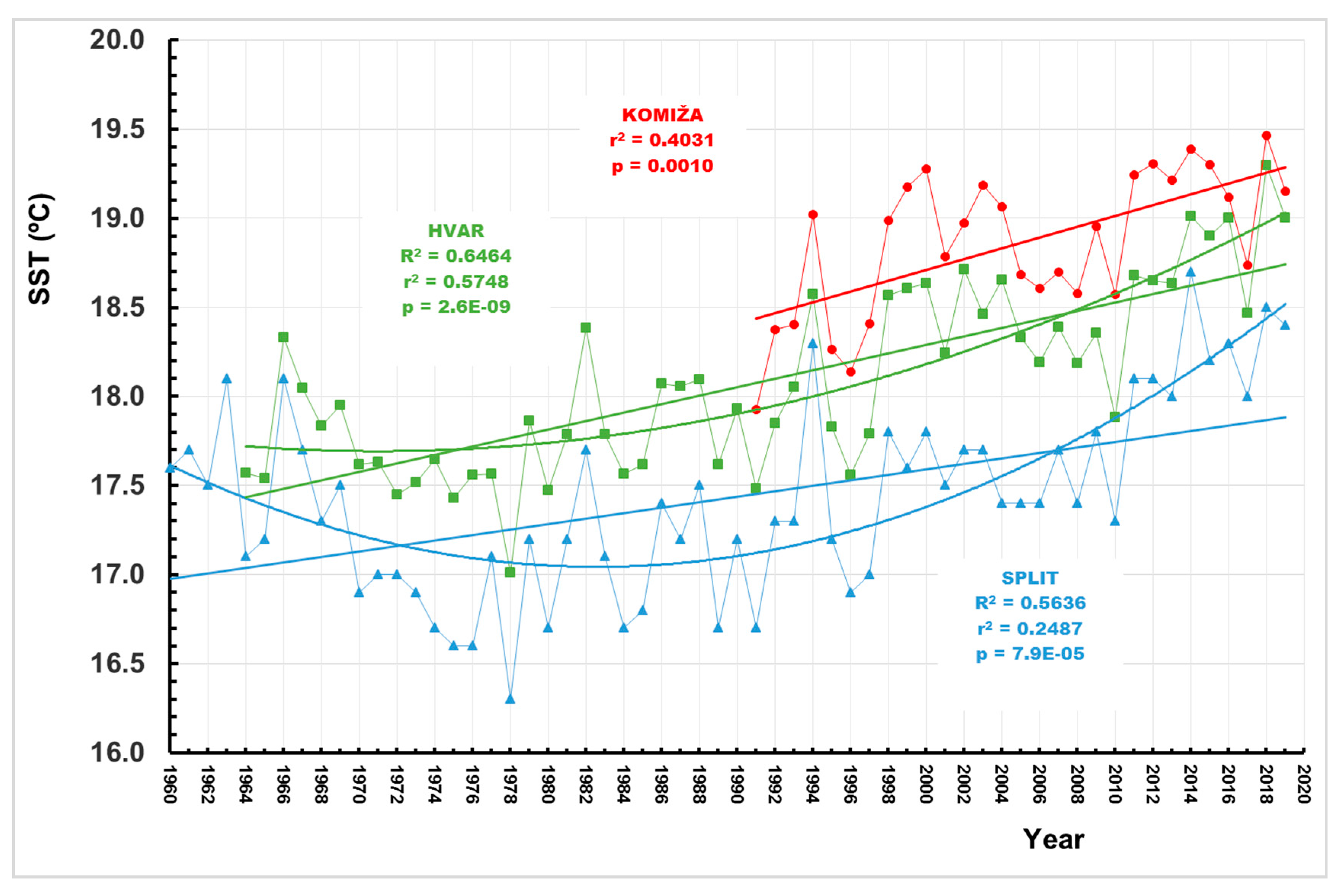
Figure 2 shows the time series of the mean annual SST measured at Split (shown in blue), Hvar (shown in green), and Komiža (shown in red) stations.
The linear regressions evidenced increasing trends in the SST at all analyzed stations, which were corroborated by the results of the M–K test (i.e., p < 0.01). However, to achieve better fitting to the data, quadratic regressions were performed on the time series of Split and Hvar stations. The results showed slightly higher R2 values than the coefficient of linear regressions r2. Quadratic regression was not performed on the time series from Komiža due to the missing data before 1991.
The RAPS method has been used on the time series of SST from all analyzed stations. The results are in the 
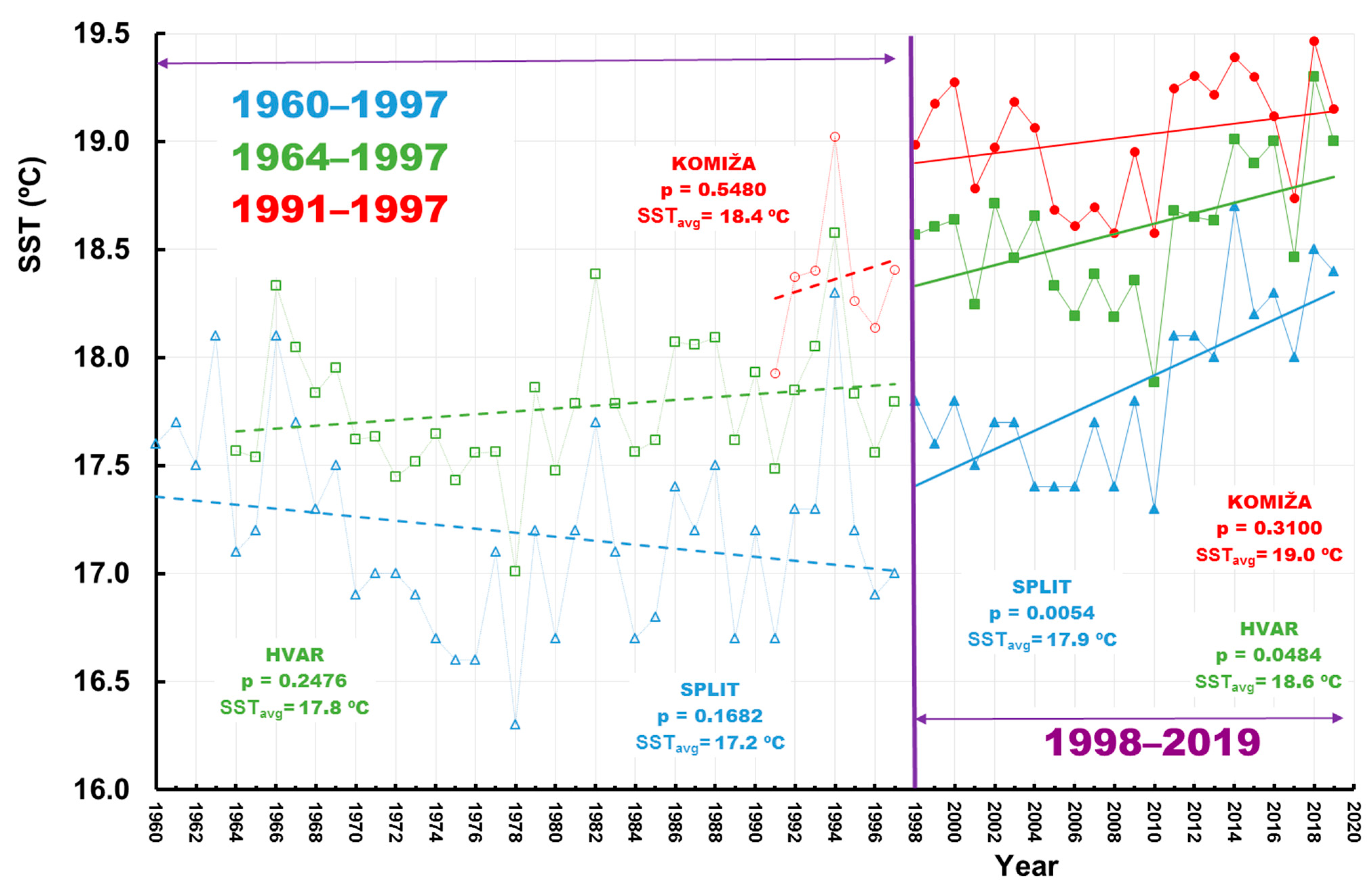
Supplementary Material (S1) and they evidenced the presence of two sub–periods: (i) from the beginning of the respective time series until 1997, and (ii) from 1998 to 2019 (Figure 3).
Despite the differences in the duration of the time series, increasing (Hvar and Komiža) or decreasing (Split) trends in SST were not statistically significant in the first sub–period defined by the RAPS (p–values > 0.05; Figure 3). Statistically significant increasing trends in the SST occurred in the second sub–period at stations in Hvar and Split (p–values < 0.05), and in Komiža there was not a statistically significant trend in the second sub–period (p–values > 0.05).
The average values of the mean annual SST within the sub–periods defined by the RAPS method are shown in Figure 3 and Table 3. The statistical analyses evidenced statistically significant differences between the average values of the mean annual SST in the two sub–periods, with the rejection of the null hypothesis of the t–test (low p–values, i.e., p < 0.01), and similar variances of the sub–periods reflecting the failure to reject the null hypothesis of the F–test (high p–value).
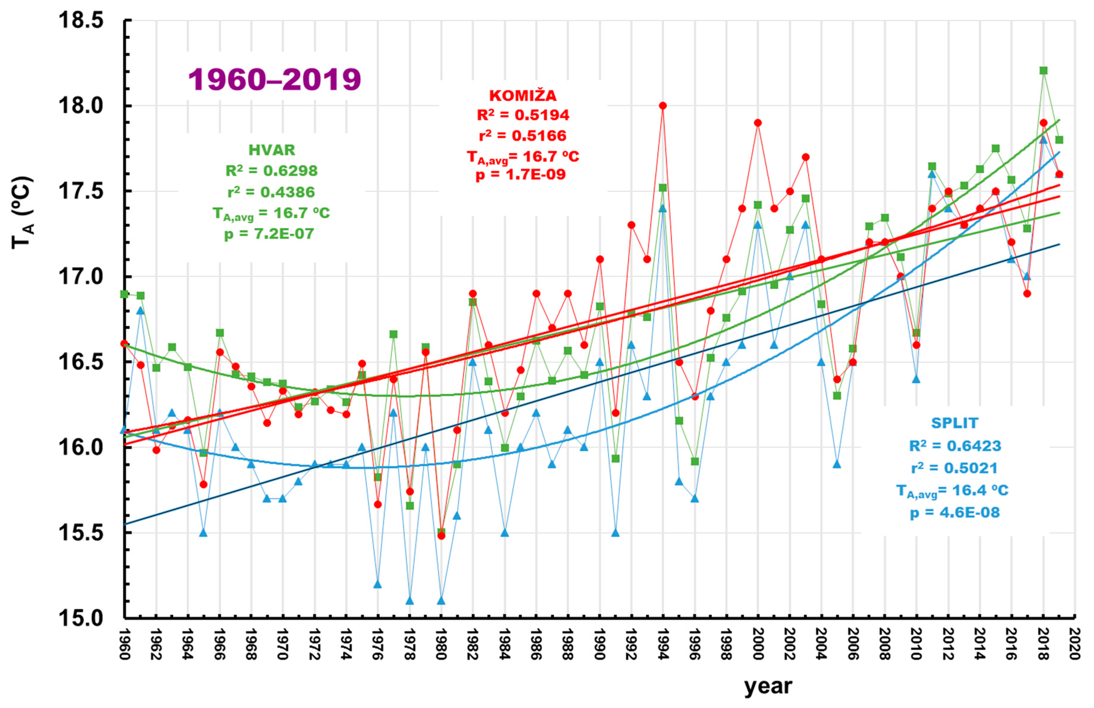
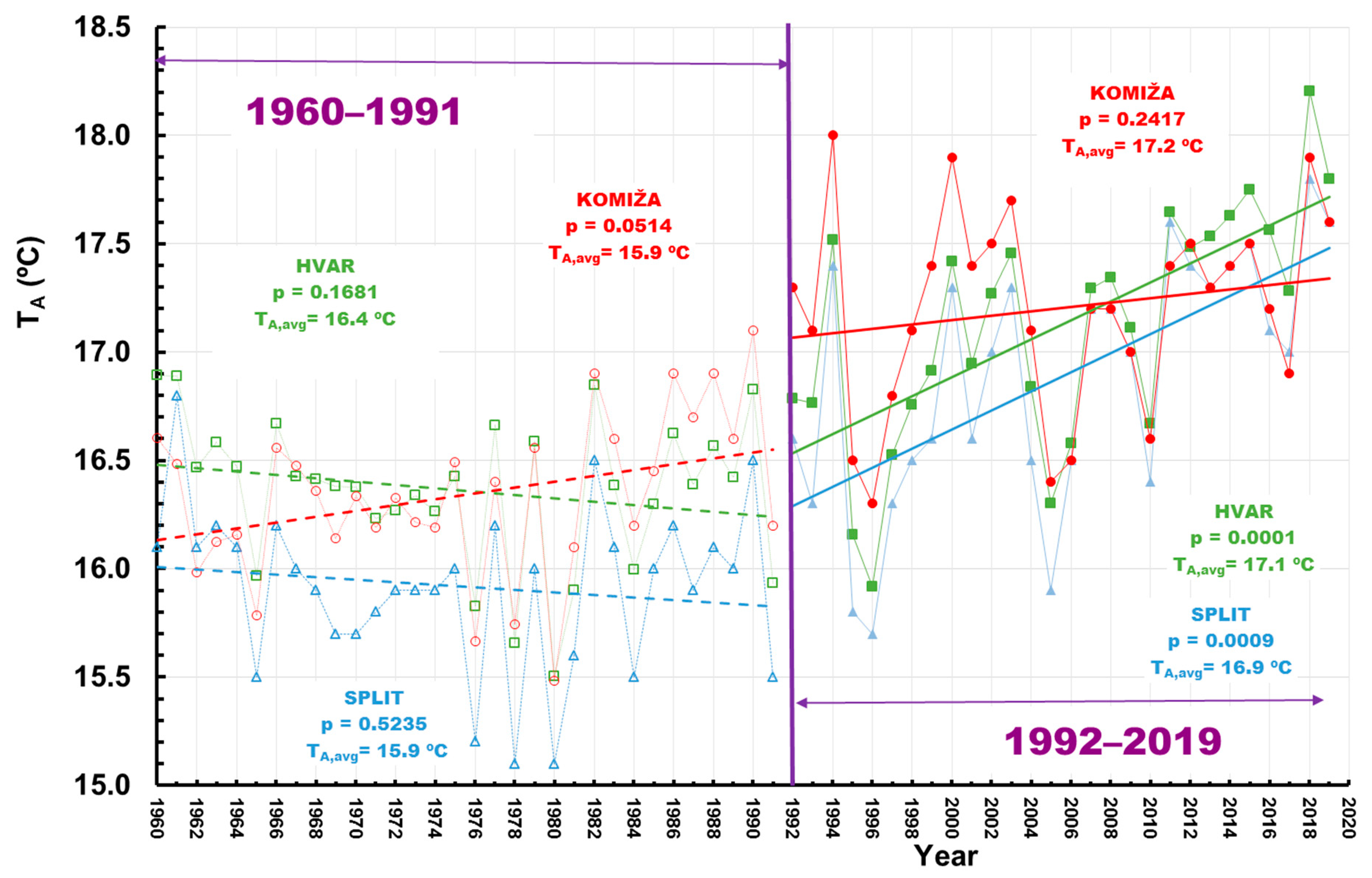
Figure 4 shows the time series of the mean annual air temperatures measured at Split, Hvar, and Komiža stations. The average values of the mean annual air temperature during the analyzed periods were identical at Hvar and Komiža (16.7 °C), while in Split they were slightly lower (16.4 °C). All three stations showed statistically significant increasing trends in the mean annual air temperature (i.e., low p–values < 0.01). To achieve better fitting to the data, quadratic regressions were preferred over simple linear regression for the time series from all analyzed stations.
The RAPS method evidenced the presence of two sub–periods in the mean annual air temperature time series: (i) 1960–1991, and (ii) 1992–2019 (Figure 5). The M–K test evidenced that the trends within the first sub–period were statistically insignificant (p–values > 0.05) at all analyzed stations. However, within the second sub–period statistically significant increasing trends were observed at Hvar and Split stations (p < 0.01).
The average values of the mean annual air temperature within a sub–period defined by the RAPS method are shown in Figure 5 and Table 4. The statistical analyses evidenced statistically significant differences between the average values the mean annual air temperature in the two sub–periods, with the rejection of the null hypothesis of the t–test (low p–values, i.e., p < 0.01), and similar variances of the sub–periods reflecting the failure to reject the null hypothesis of the F–test (high p–value). The results indicated that the air temperature had started to increase considerably at the beginning of the 1990s at all analyzed stations. These results fit the regional warming patterns observed in Croatia and the western Balkans [22,23,24,25]. Furthermore, it can be concluded that the rapid increase in air temperature had occurred 6 years before the increase in SST at all analyzed stations.
The correlation between the mean annual SST and the mean annual air temperature time series was the highest in Hvar, with the values of r2 = 0.796 in the period from 1964 to 2019, followed by Split with r2 = 0.688 in the period from 1960 to 2019, and the lowest was in Komiža with r2 = 0.6183 in the period from 1991 to 2019.
Table 5 shows the r–squared values of the linear correlation coefficients (i) between the pairs of the time series of the mean annual SST during periods of contemporaneous measurements at all three stations (from 1991 to 2019), and (ii) between the pairs of the time series of the mean annual air temperature (from 1960 to 2019).
The high values of r2 indicated the similarity of the SST and the air temperature regimes at analyzed stations. The highest r2 from the SST time series was observed between the closest stations, Komiža and Hvar, r2 = 0.87, and the lowest between Komiža and Split, r2 = 0.75. The highest r2 value from the time series of the mean annual air temperature was observed between Split and Hvar stations, r2 = 0.95, and the lowest between Hvar and Komiža, r2 = 0.80.
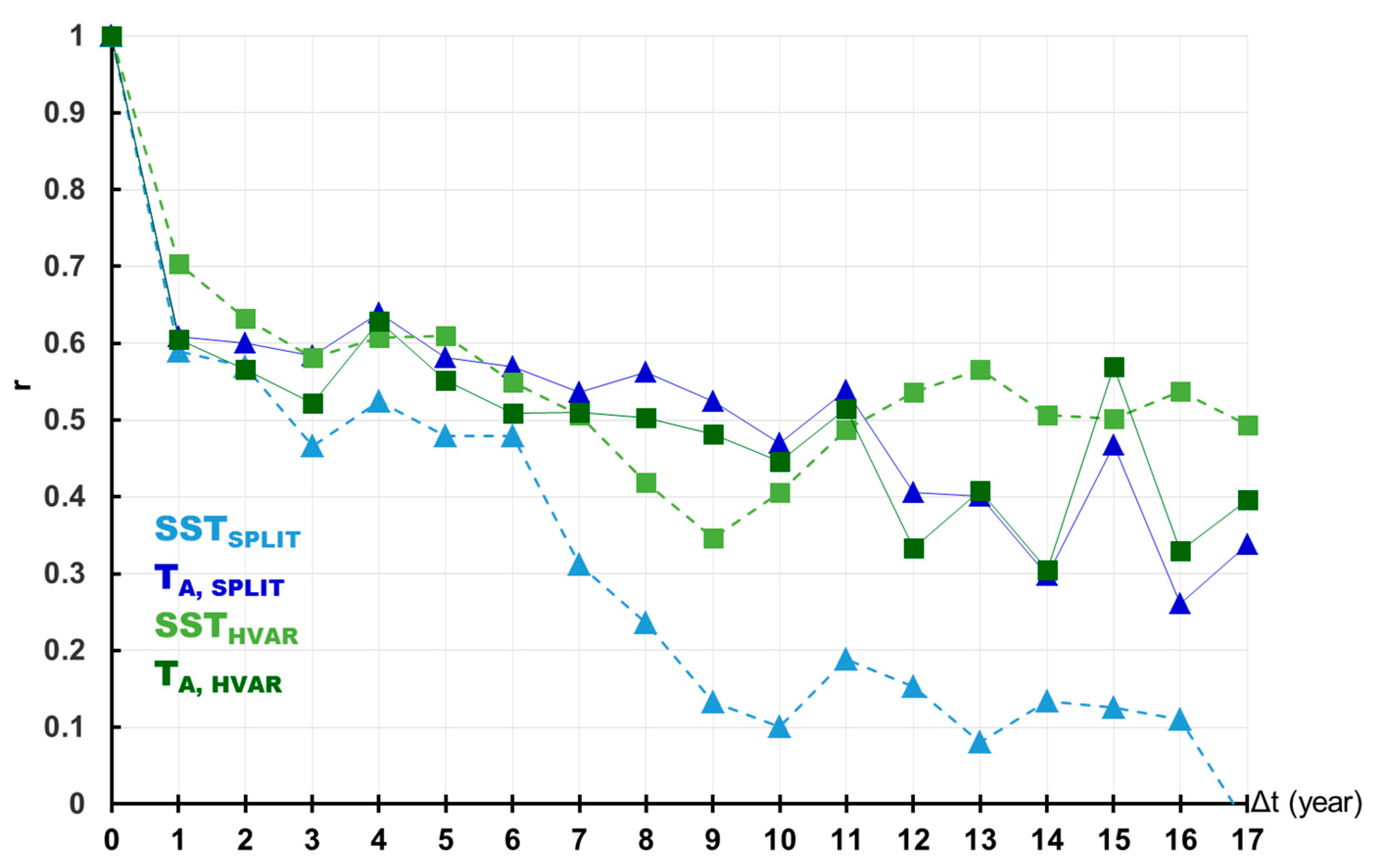
Furthermore, the autocorrelation method was performed on the time series of the mean annual SST and air temperature measured at Split and Hvar stations, for the period from 1960 to 2019, and from 1964 to 2019, respectively. The time series from Komiža did not qualify for autocorrelation due to the insufficient duration of the time series of SST (from 1991 to 2019). The results indicated the similar behavior of the SST and the air temperature in Hvar and the air temperature in Split having a long–term autocorrelation (Figure 6). However, the autocorrelogram of the SST from the Split station is significantly different. The values of r were steady at approximately 0.5 until 6 years when a significant drop occurred. After 8 years, the values of the autocorrelation coefficient were lower than the significance threshold (0.2) meaning that the “memory of the system” was lost. Plausible causes that decreased the correlation of the time series of the mean annual SST include higher variability of SST in Split, pronounced coastal effect and local variability of climate, and bay–like topography. Considering spatially and temporally limited data measured at the station in Split, a more detailed study should be conducted to evaluate the driving force of this different behavior.

4.2. Analyses of the Mean Monthly Sea Surface Temperature and Air Temperature

The summary of the statistical analysis (minimum, average, maximum, and range) of the mean monthly SST and air temperature (TA) time series, as well as their differences (ΔT = SST–TA), is shown in 
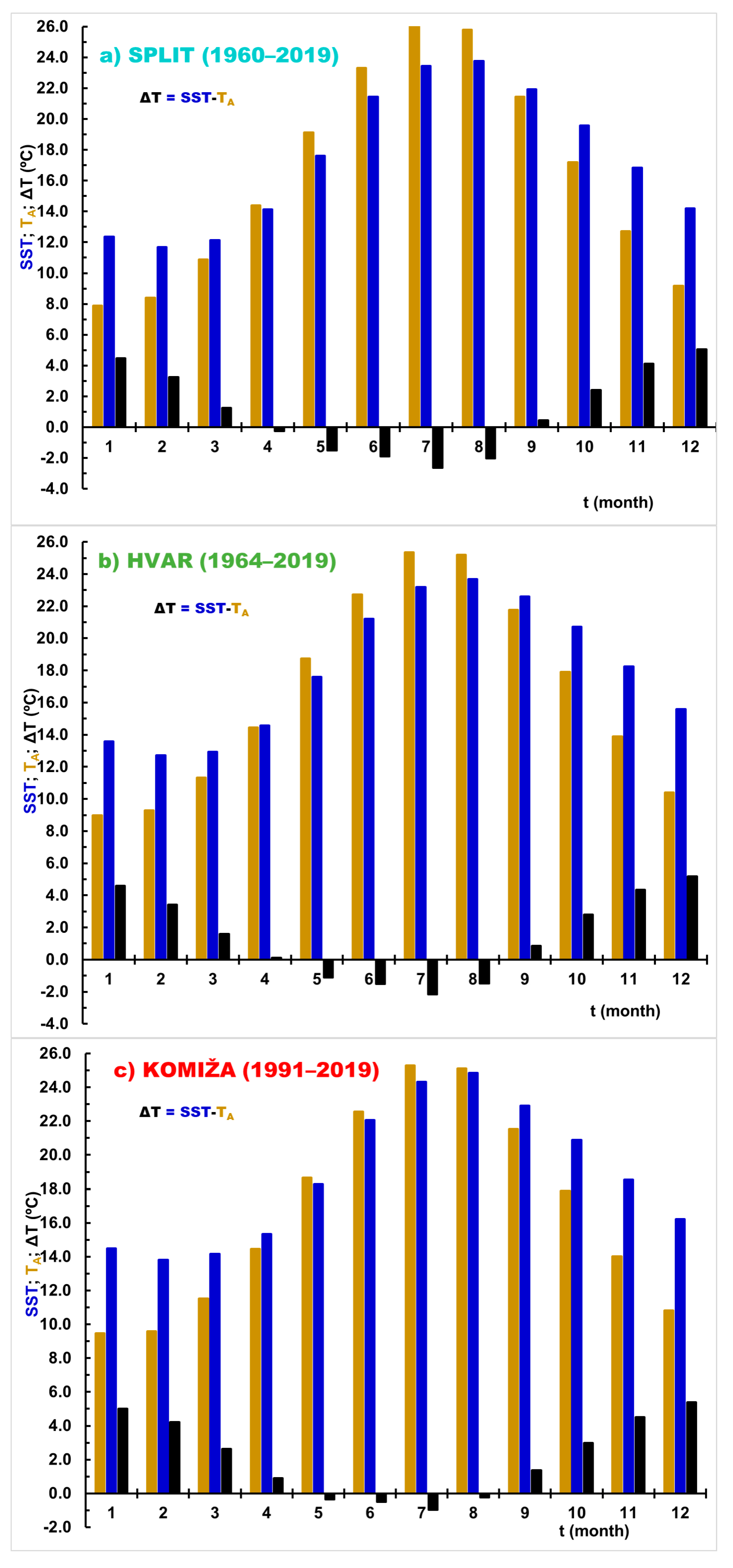
Table S2 of the supplementary material. The statistical analyses evidenced that the ΔT of the minimum values coincided at all three stations during the warmer period of the year (i.e., from May to August), and ranged from ‒1.8 to 6.4 °C in Split, from ‒2.6 to 7 °C in Hvar, and from ‒1.8 to 7 °C in Komiža. The amplitude was slightly higher at island stations (i.e., Hvar and Komiža) than at the Split station. The ΔT of the maximum values were the lowest during the warmer period of the year (from April to September) and the highest during December at all three stations, and ranged from ‒4.6 to 5.3 °C in Split, from ‒3.1 to 5 °C in Hvar, and from ‒2.8 to 4.7 °C in Komiža. The distribution of the ΔT of the average values showed a similar pattern as the ΔT of minimum and maximum, and the values were the lowest in July and the highest in December at all analyzed stations. The ΔT of the average values ranged from –2.6 to 5 °C in Split, from ‒2.2 to 5.2 °C in Hvar, and from ‒1.6 to 5.1 °C in Komiža. The ranges of the mean monthly ΔT values were the lowest (i.e., highest negative values) during the winter period (from January to March), and the highest during warmer periods of the year at all analyzed stations. The ranges of the ΔT values were from ‒4.4 to ‒0.8 °C in Split, from ‒4.1 to ‒0.2 °C in Hvar, and from ‒3.7 to ‒0.8 °C in Komiža. At all analyzed stations, the ranges of the mean monthly air temperature were significantly higher than the ranges of the SST in each month of the year.
The average values of the mean monthly SST, air temperature, as well as their difference (ΔT = SST–TA), are shown in Figure 7.
Figure 7 shows the comparison of the average values of the mean monthly SST and air temperatures at Split, Hvar, and Komiža stations. In the warmer part of the year (from May to August), the air temperature was higher than the SST at all analyzed stations. Furthermore, the air temperature and the SST were nearly identical in April at stations in Split and Hvar. The most significant difference occurred in July when their difference was 2.64 °C in Split, 2.25 °C in Hvar, and 1.63 °C in Komiža. In the colder parts of the year, the SST was higher than the air temperature at all analyzed stations, with the highest difference in December, when the mean monthly SST was on average 5 °C higher than the mean monthly air temperature. The results evidenced a very similar behavior of temperature at all analyzed stations, despite the differences in the duration of the time series. The smallest ΔT values were observed at the station in Komiža, and the highest at the Split station. This fact could be partly explained by the differences in the duration of the time series, but also by the local effect of the position of the meteorological station and its distance from the SST measuring point. Furthermore, the position of the meteorological station in terms of the distance from the landmass also plays an important role.
Table 6 shows the slope of the linear equation, a, squared values of the linear correlation coefficient, r2, and M–K probability values, p, for the analyzed time series of the mean monthly SST. The results indicated that the statistically significant increasing trends in SST were observed in the warmer parts of the year (March–August) in Split, throughout the year in Hvar, while the statistically more complex situation was observed in Komiža, where increasing trends occurred in March, June, July, September, and December.
Table 7 shows the slope of the linear equation, a, squared values of the linear correlation coefficient, r2, and M–K probability values, p, calculated from the time series of the mean monthly air temperature. The results indicated the nearly identical behavior of the air temperature at all analyzed stations. Statistically significant increasing trends in the mean monthly air temperature occurred from March to August at all analyzed stations, but also in December at the Split and Komiža stations.
Statistical analyses performed on the time series of the mean monthly SST and air temperature undoubtedly evidenced that the most significant increasing trends in the SST and the air temperature occurred during warmer parts of the year, i.e., during spring and summer. Similar warming trends could be present over the entire Adriatic Sea and its coast, but further detailed studies on the time series from the other meteorological stations, coupled with studies using gridded datasets from remote sensing or numerical simulation, are needed to assess whether these trends are present on a regional scale. Furthermore, the results of this study are in concordance with findings from Bartolini et al. [23], who conducted a regional climatological study where they analyzed air temperatures at 21 stations in the Mediterranean region, i.e., in Tuscany, Italy, and they have concluded that the most rapid and intensive warming trends occurred from March to August.
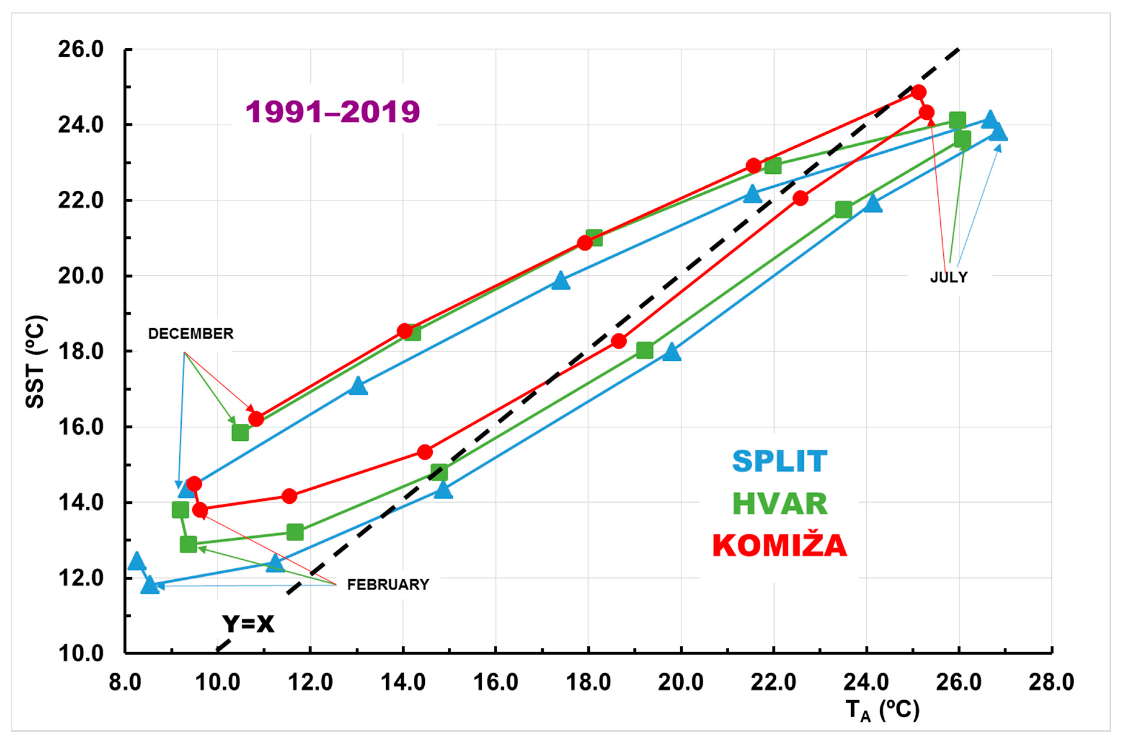
Figure 8 shows the ratio of the average values of the mean monthly SST and air temperature in the period of contemporaneous measurements at all three stations (from 1991 to 2019). The data loops from all three stations are similar in shape but are slightly shifted in values. The analyses of the time series from the period of contemporaneous measurements confirmed the previous conclusion which was based on the divergent time series.

5. Conclusions

In the past 40 years, the Adriatic Sea and adjacent coastal areas have faced an increase in sea surface temperature, air temperature, and changes in the precipitation regime. Statistical analyses conducted within this study evidenced increasing trends in both the investigated temperature time series (i.e., SST and TA). The results of RAPS indicated that the increase has been sharper since the 1990s but it occurred with a significant temporal shift (6 years) between the mean annual air temperature and SST. The observed lag in the warming of the Adriatic Sea is most likely a result of the slower response of the sea to the warming process, due to the inherent ability of the sea to absorb vast amounts of energy. Furthermore, the most significant increasing trends in the mean monthly air temperature and SST occurred during warmer parts of the year, i.e., during spring and summer. These results are in accordance with regional climate models [25,26] for the Adriatic Sea.
The climate changes described in this and other works (e.g., [22,23,24]) have a strong impact on the environment, the marine species, and the population living in the Adriatic region. For example, the habitats of many thermophilic species had migrated horizontally and vertically towards the deeper and the colder parts of the sea. If the sea surface temperature will continue to increase, the geographical distribution of these species will continue to decrease and will eventually cause extirpation and possibly even extinction. In addition, changes in the composition and quantity of zooplankton were observed, particularly in coastal areas of the Adriatic. Moreover, frequent blooms of marine phytoplankton and the spread of bacteria and thermophilic species of tropical algae were also observed [4].
Regional climate models for the Mediterranean region showed the continuation or even an increase in warming trends, and therefore, it is realistic to assume that the negative changes in the Adriatic Sea and its coast will be even more pronounced in the near future. In conjunction with increasing anthropogenic pressures, such as overfishing, urban and industrial pollution, the devastation of habitats, seasonal tourism pressures, and hydrocarbon exploitation, the negative consequences could be even more drastic. The lack of reliable indicators of climate change or variability, i.e., the sea surface and the air temperature, measured over a dense network of meteorological stations, has a significant influence on the development of effective measures for mitigation of negative effects of climate change [27].
Furthermore, as a result of the variable distance from the mainland, and local or regional topography, the effects of climate change manifest differently in specific islands or coastal regions. Limited and vulnerable groundwater resources along the coast of the Croatian part of the Adriatic Sea and in the related islands, in combination with unsustainable anthropic activities (e.g., mass tourism, land–use changes, groundwater over–abstraction, and urbanization), significantly reduce the options for adaption to current and future climate change. Due to the vast cultural, historical, social, geographical, and biological diversity, the Mediterranean region requires urgent and effective measures that will foster its sustainable development. The fundamental problem is that the Croatian part of the Adriatic Sea, similar to the other countries in the Mediterranean region, does not have a sufficiently dense network of meteorological stations and sufficiently long time series of measured data, especially sea surface temperature data.
The availability of high–resolution data on climate change and variability could enable island communities to enhance their resilience and design site–specific measures to mitigate possible negative effects on water availability and natural ecosystems. Besides the structural modifications (e.g., re–use of purified domestic and industrial wastewater, reduction in losses from water supply systems, desalinization plants, managed aquifer recharge), a holistic approach could also be fostered by increasing awareness and education of the local population on correct utilization of the water resource (e.g., promotion of water savings during dry months, rainwater harvesting, planting of crops that require little or no irrigation, reduction in carbon footprint, and preservation of ecosystems and their services to mitigate floods and droughts).
The authors hope that this study will contribute to a better understanding of this topic and that it will initiate interdisciplinary cooperation and discussion on the more intensive and coordinated investigation of this complex and exceedingly important issue for Croatia, the Adriatic, and the Mediterranean region.

Supplementary Materials

The following are available online at https://www.mdpi.com/article/10.3390/jmse9040358/s1. The following Supplementary Materials are submitted alongside the manuscript: Figure S1a. The RAPS visualization of the mean annual SST time series; Figure S1b. The RAPS visualization of the mean annual air temperature time series; Table S2. Statistics (minimum, average, maximum, and range) of the mean monthly SST, air temperature (TA), and their difference (ΔT = SST-TA) from the time series measured at Split, Hvar, and Komiža stations. The negative values of ΔT were highlighted in red.

Author Contributions

Conceptualization, investigation, and writing of original draft, O.B.; investigation, visualization, and data curation, D.B.; data curation and validation, review and editing, M.P. (Matko Patekar); supervision, writing and editing, and validation, M.P. (Marco Pola). All authors have read and agreed to the published version of the manuscript.

Funding

This research was supported by the Croatian Geological Survey, Department of Hydrogeology and Engineering Geology.

Institutional Review Board Statement

Not applicable.

Informed Consent Statement

Not applicable.

Data Availability Statement

The data used within this study are the property of the Croatian Meteorological and Hydrological Service (DHMZ). Terms of use, data availability, and contact can be found at: https://klima.hr/razno/katalog_i_cjenikDHMZ.pdf.

Acknowledgments

Data used in this study was provided by courtesy of the Croatian Meteorological and Hydrological Service, for which we thank them.

Conflicts of Interest

The authors declare no conflict of interest.

References

  1. Viličić, D. Jadran i globalne promjene [The Adriatic and the global changes]. Priroda 2013, 13, 22–28. [Google Scholar]
  2. Viličić, D. Specifična oceanološka svojstva hrvatskog dijela Jadrana [Specific oceanographic characteristics of the Croatian part of The Adriatic Sea]. Hrvatske Vode 2013, 22, 297–314. [Google Scholar]
  3. Grbec, B.; Morović, M.; Matić, F.; Ninčević Gladan, Ž.; Marasović, I.; Vidjak, O.; Bojanić, N.; Čikeš Keč, V.; Zorica, B.; Kušpilić, G.; et al. Climate regime shifts and multi-decadal variability of the Adriatic Sea pelagic ecosystem. Acta Adriatica 2015, 56, 47–66. [Google Scholar]
  4. Krželj, M. Utjecaj klimatskih promjena na morski okoliš [Climate change effects on the marine environment]. Paediatr. Croat. 2010, 54, 18–23. [Google Scholar]
  5. Orlić, M. Croatian coastal waters. In Physical Oceanography of the Adriatic Sea: Past, Present and Future; Cushman-Roisin, B., Gačić, M., Poulain, P.-M., Artegiani, A., Eds.; Kluwer Academic Publishers: Dordrecht, The Netherlands, 2001; pp. 189–214. [Google Scholar]
  6. Bonacci, O.; Ljubenkov, I. Različite vrijednosti i trendovi temperatura zraka na dvije postaje na malom otoku: Slučaj meteoroloških postaja Korčula i Vela Luke na otoku Korčuli [Different values and air temperature trends at meteorological stations on small island of Korčula: Case study of meteorological stations in Vela Luka and Korčula]. Hrvat. Vode 2019, 28, 183–196. [Google Scholar]
  7. Bonacci, O.; Patekar, M.; Pola, M.; Roje-Bonacci, T. Analyses of climate variations at four meteorological stations on remote islands in the Croatian part of the Adriatic Sea. Atmosphere 2020, 11, 1044. [Google Scholar] [CrossRef]
  8. Vlahakis, G.N.; Pollatou, R.S. Temporal variability and spatial distribution of Sea Surface Temperatures in the Aegean Sea. Theor. Appl. Climatol. 1993, 47, 15–23. [Google Scholar] [CrossRef]
  9. Bulgin, C.E.; Merchant, C.J.; Ferreira, D. Tendencies, variability and persistence of sea surface temperature anomalies. Sci. Rep. 2020, 10, 7986. [Google Scholar] [CrossRef] [PubMed]
  10. Penzar, B.; Penzar, I.; Orlić, M. Vrijeme i Klima Hrvatskog Jadrana (Weather and Climate of the Croatian Adriatics), 1st ed.; Dr. Frletar: Zagreb, Croatia, 2001. [Google Scholar]
  11. Duplančić Leder, T.; Ujević, T.; Čala, M. Coastline lengths and areas of islands in the Croatian part of the Adriatic Sea determined from the topographic maps at the scale 1:25,000. Geoadria 2004, 9, 5–32. [Google Scholar]
  12. Šegota, T.; Filipčić, A. Köppenova podjela klima i hrvatsko nazivlje [Köppen climate classification and the Croatian nomenclature]. Geoadria 2003, 8, 17–37. [Google Scholar] [CrossRef] [Green Version]
  13. Pandžić, K. Naputak za Opažanja i Mjerenja na Glavnim Meteorološkim Postajama (Instructions for Observation and Measurements at Main Meteorological Stations); Državni hidrometeorološki zavod: Zagreb, Croatia, 2008. [Google Scholar]
  14. Heino, R. Climate in Finland during the period of meteorological observations. Finn. Meteorol. Inst. Contrib. 1994, 12, 209. [Google Scholar]
  15. Bonacci, O.; Željković, I.; Trogrlić, R.Š.; Milković, J. Differences between true mean daily, monthly and annual air temperatures and air temperatures calculated with three equations: A case study from three Croatian stations. Theor. Appl. Climatol. 2013, 114, 271–279. [Google Scholar] [CrossRef]
  16. Gough, W.A.; Žaknić-Ćatović, A.; Zajch, A. Sampling frequency of climate data for the determination of daily temperature and daily temperature extrema. Int. J. Climatol. 2020, 40, 5451–5463. [Google Scholar] [CrossRef] [Green Version]
  17. Husain Shourov, M.M.; Mahmud, I. pyMannKendall: A python package for non parametric Mann Kendall family of trend tests. J. Open Source Softw. 2019, 4, 1556. [Google Scholar] [CrossRef]
  18. Garbrecht, J.; Fernandez, G.P. Visualization of trends and fluctuations in climatic records. Water Resour. Bull. 1994, 30, 297–306. [Google Scholar] [CrossRef]
  19. Bonacci, O.; Roje-Bonacci, T. Primjena metode dan za danom (day to day) varijabilnosti temperature zraka na podatcima opaženim na opservatoriju Zagreb-Grič (1887–2018). Hrvat. Vode 2019, 28, 125–134. [Google Scholar]
  20. McGhee, J.W. Introductory Statistics; West Publishing Company: Saint Paul, MN, USA, 1985. [Google Scholar]
  21. Mangin, A. Pour une meilleure connaissance des systemes hydrologiques a partir des analyses correlatioire et spectrale. J. Hydrol. 1984, 67, 25–43. [Google Scholar] [CrossRef]
  22. Bonacci, O. Analiza nizova srednjih godišnjih temperature zraka u Hrvatskoj. Građevinar 2010, 62, 781–791. [Google Scholar]
  23. Bonacci, O. Increase of mean annual surface air temperature in the Western Balkans during last 30 years. Vodoprivreda 2012, 44, 75–89. [Google Scholar]
  24. Bartolini, G.; di Stefano, V.; Maracchi, G.; Orlandini, S. Mediterranean warming is especially due to summer season–Evidences from Tuscany (central Italy). Theor. Appl. Climatol. 2012, 107, 279–295. [Google Scholar] [CrossRef]
  25. Branković, Č.; Güttler, I.; Gajić-Čapka, M. Evaluating climate change at the Croatian Adriatic from observations and regional climate models’ simulations. Clim. Dyn. 2013, 41, 2353–2373. [Google Scholar] [CrossRef]
  26. Pandžić, K.; Kobold, M.; Oskoruš, D.; Biondić, B.; Biondić, R.; Bonacci, O.; Likso, T.; Curić, O. Standard normal homogeneity test as a tool to detect change points in climate-related river discharge variation: Case study of the Kupa River Basin. Hydrol. Sci. J. 2020, 65, 227–241. [Google Scholar] [CrossRef]
  27. Al Sayah, M.J.; Abdallah, C.; Khouri, M.; Nedjai, R.; Darwich, T. A framework for climate change assessment in Mediterranean data-sparse watersheds using remote sensing and ARIMA modeling. Theor. Appl. Climatol. 2020, 143. [Google Scholar] [CrossRef]
Figure 1. Map of the study area showing the locations of the three meteorological stations whose data were analyzed in this study.
Jmse 09 00358 g001
Figure 2. Time series of the mean annual SST measured at Split, Hvar, and Komiža stations. The r2 and R2 represent the r–squared values of the correlation coefficients of the linear and quadratic regressions, respectively, and p represents the Mann–Kendall (M–K) test values.
Jmse 09 00358 g002
Figure 3. Time series of the mean annual SST measured at Split, Hvar, and Komiža stations. SSTavg is an average value of the mean annual SST, and p represents M–K test values, calculated for two sub–periods defined by the results of Rescaled Adjusted Partial Sums (RAPS) method.
Jmse 09 00358 g003
Figure 4. Time series of the mean annual air temperature measured at Split, Hvar, and Komiža stations. The r2 and R2 represent the square values of the correlation coefficients of the linear and quadratic regressions, respectively, and p represents M–K test values. TA, avg is the average value of the mean annual air temperature in the investigated period.
Jmse 09 00358 g004
Figure 5. Time series of the mean annual air temperature measured at Split, Hvar, and Komiža stations. TA, avg is an average value of the mean annual air temperature, and p represents M–K test values, calculated for two sub–periods defined by the results of RAPS.
Jmse 09 00358 g005
Figure 6. Autocorrelogram of the mean annual SST and the air temperature (TA) time series measured at stations in Split (blue) and Hvar (green). Δt refers to the year in a sequence.
Jmse 09 00358 g006
Figure 7. The average values of the monthly mean SST (blue), air temperature (brown), as well as their difference ΔT = SST-TA (black) from the time series measured at Split (a), Hvar (b), and Komiža (c) stations.
Jmse 09 00358 g007
Figure 8. The ratio of the mean monthly SST and air temperature from the period of contemporaneous measurements at all three analyzed stations.
Jmse 09 00358 g008
Table 1. Characteristics of the investigated meteorological stations.
SplitHvarKomiža
Latitude43°30′30″43°10′16″43°02′54″
Longitude16°25′35″16°26′13″16°05′07″
H (m a.s.l.)1222020
Investigated period (SST)1960–20191964–20191991–2019
Investigated period (TA)1960–20191960–20191960–2019
L (m)3100 100190
Ls (m)51580175
Note: H—the altitude of the meteorological station; SST—sea surface temperature; TA—air temperature; L—the distance between the SST and the air temperature measuring point; Ls—minimum distance between meteorological stations and the seashore.
Table 2. Statistics (minimum, average, maximum) of the mean annual SST, air temperature (TA), and their difference (ΔT = SST-TA).
T (°C)SPLITHVARKOMIŽA
1960−20191964−20191991−2019
SSTMinimum16.3 17.0 17.9
Average17.418.118.9
Maximum18.7 19.3 19.5
Range2.42.31.6
TAMinimum15.1 15.5 16.2
Average16.416.717.2
Maximum17.8 18.2 18.0
Range2.72.71.8
ΔTMinimum1.21.51.7
Average1.11.41.7
Maximum0.91.11.5
Range-0.3-0.4-0.2
Table 3. The average values of the mean annual SST time series within a sub–period defined by the RAPS method at the analyzed stations and the results of the F–test and the t-test.
StationSub–PeriodSSTavg (°C)p (F–test)p (t-test)
SPLIT1960–199717.190.5652.8 × 10−7
1998–201917.85
HVAR1964–199717.770.7887.7 × 10−13
1998–201918.58
KOMIŽA1991–199718.350.4782.0 × 10−5
1998–201919.02
Table 4. The average values of the mean annual air temperature time series within a sub–period defined by the RAPS method at the analyzed stations and the results of the F–test and the t–test.
StationSub–PeriodTA,avg(°C)p (F–Test)p (t–Test)
SPLIT1960–199115.980.6643.4 × 10−11
1992–201917.03
HVAR1960–199116.400.4151.6 × 10−10
1992–201917.26
KOMIŽA1960–199116.450.3317.8 × 10−9
1992–201917.26
Table 5. Matrix table of the r–squared values of the linear correlation coefficients, r2, calculated from the time series of the mean annual SST and the mean annual air temperature.
Sea Surface Temperature (1991–2019)
r2SPLITHVARKOMIŽA
SPLIT10.8690.751
HVAR 10.872
KOMIŽA 1
Air Temperature (1960–2019)
r2SPLITHVARKOMIŽA
SPLIT10.9570.816
HVAR 10.806
KOMIŽA 1
Table 6. The slope of the linear equation, a, squared values of the linear correlation coefficient, r2, and M–K probability values, p, calculated from the time series of the mean monthly SST. M–K p values 0.01 < p < 0.05 are highlighted in blue, and p < 0.01 in red.
MonthSplitHvarKomiža
ar2par2par2p
10.0070.0210.4580.0180.1950.0020.0230.0920.137
20.0100.0680.1730.0150.1610.0040.0190.0980.220
30.0170.1290.0100.0210.2220.0000.0250.1500.061
40.0160.1210.0020.0230.2767.5 × 10−50.0530.4687.5 × 10−5
50.0230.1090.0300.0300.2160.0010.0300.0690.309
60.0240.1630.0020.0350.2954.5 × 10−50.0370.1140.036
70.0240.2171 × 10−40.0340.3617.4 × 10−60.0400.2200.016
80.0190.1150.0090.0280.2720.0000.0180.0320.347
90.0140.0470.0710.0210.1140.0090.0350.0800.034
100.0100.0290.1130.0180.0870.0360.0012 × 10−40.820
110.0110.0330.1400.0200.1270.0060.0310.0980.067
120.0080.0230.1360.0220.1920.0010.0510.2430.008
Table 7. The r–squared values of the linear correlation coefficient, r2, slope of the linear equation, a, and M–K probability values, p, calculated from the time series of mean monthly air temperature. M–K p values 0.01 < p < 0.05 are highlighted in blue, and p < 0.01 in red.
MonthSplitHvarKomiža
ar2par2par2p
10.0190.0440.1470.0110.0180.3780.0190.0560.100
20.0150.0200.3040.0100.0110.4630.0140.0260.277
30.0280.0860.0380.0220.0790.0390.0220.0860.037
40.0320.1520.0010.0220.1200.0010.0230.1310.002
50.0270.0890.0140.0250.1150.0030.0240.1030.011
60.0480.3201.2 × 10−50.0420.3298.6 × 10−80.0400.3173.9 × 10−6
70.0490.4029.4 × 10−70.0460.4706.9 × 10−80.0430.3954.1 × 10−7
80.0500.2665.3 × 10−50.0440.3363.1 × 10−60.0460.3085.2 × 10−6
90.0120.0200.2550.0160.0460.0970.0150.0420.109
100.0140.0400.1690.0090.0180.3920.0140.0410.203
110.0190.0530.1030.0140.0310.1840.0210.0750.050
120.0170.0550.0450.0060.0070.3500.0170.0630.039
Publisher’s Note: MDPI stays neutral with regard to jurisdictional claims in published maps and institutional affiliations.

