Article

Multicriteria Ship Route Planning Method Based on Improved Particle Swarm Optimization–Genetic Algorithm

State Key Laboratory on Integrated Optoelectronics, College of Electronic Science and Engineering, Jilin University, Changchun 130000, China
*
Author to whom correspondence should be addressed.
J. Mar. Sci. Eng. 2021, 9(4), 357; https://doi.org/10.3390/jmse9040357
Submission received: 28 February 2021 / Revised: 13 March 2021 / Accepted: 19 March 2021 / Published: 25 March 2021
(This article belongs to the Special Issue Automatic Control and Routing of Marine Vessels)

Abstract

:
With the continuous prosperity and development of the shipping industry, it is necessary and meaningful to plan a safe, green, and efficient route for ships sailing far away. In this study, a hybrid multicriteria ship route planning method based on improved particle swarm optimization–genetic algorithm is presented, which aims to optimize the meteorological risk, fuel consumption, and navigation time associated with a ship. The proposed algorithm not only has the fast convergence of the particle swarm algorithm but also improves the diversity of solutions by applying the crossover operation, selection operation, and multigroup elite selection operation of the genetic algorithm and improving the Pareto optimal frontier distribution. Based on the Pareto optimal solution set obtained by the algorithm, the minimum-navigation-time route, the minimum-fuel-consumption route, the minimum-navigation-risk route, and the recommended route can be obtained. Herein, a simulation experiment is conducted with respect to a container ship, and the optimization route is compared and analyzed. Experimental results show that the proposed algorithm can plan a series of feasible ship routes to ensure safety, greenness, and economy and that it provides route selection references for captains and shipping companies.

1. Introduction

With the progress of navigation technology, the safety and energy-saving problems associated with maritime navigation have gradually become the focus of human attention. Severe winds, waves, and other meteorological factors seriously affect the safety of ships when sailing at sea. Currently, the weather forecasting technology has rapidly developed. The weather forecast information can be used to plan routes for ships to avoid severe winds and waves. Recently, the International Maritime Organization (IMO) and governments have paid close attention to the air pollution and energy consumption of ships. In 2018, the IMO adopted the “preliminary strategy for greenhouse gas emission reduction of IMO ships,” thereby sending a strong signal to the international community that the shipping industry is turning into a low-carbon industry [1]. The reduction of fuel consumption and carbon emissions through reasonable route planning is an important measure in response to the low-carbon strategy. To plan an efficient route, the captain must completely utilize the weather forecast data according to the voyage mission and characteristics of the ship and avoid selecting high-risk routes against winds and waves. The following elements must be fully considered when planning multicriteria ship routes.
  • The navigation time of the ship must be reduced.
  • The fuel consumption of ships must be reduced.
  • Areas with severe sea conditions must be avoided, ship rolling must be reduced, and the safety of ships and cargo must be ensured.
In the case of the first element, regardless of ship stalls and weather risks, the great circle route is an ideal route because of the short voyage, thereby reducing the navigation time [2]. The main method for realizing the second element is to select the economic route. The main method for realizing the third element is to select safe routes that avoid areas with high meteorological risks based on weather forecast data and ship characteristics. The prosperity and development of shipping can be further promoted by finding an appropriate methodology to comprehensively consider the three elements to design reasonable, safe, and green alternative routes for ships.
Currently, with the rapid development of the optimization theory, some single-criteria and multicriteria route planning algorithms for ships have been proposed. Initially, some traditional mathematical methods were applied to solve the problem of ship route planning.
For example, James applied the isochron method to solve the problem of ship route planning under meteorological conditions [3]. However, this method has the “isochron loop” problem, making it unsuitable for computer-aided calculation. To solve this problem, Hagiwara et al. proposed a modified isochron method [4], and Lin et al. proposed a three-dimensional modified isochron method [5]. These two methods consider minimum fuel consumption and minimum navigation time as optimization goals. The route is optimized, but there is still a problem of complex calculations. Smierzchalski et al. used the isochron method for generating the initial route and used the evolutionary algorithm to obtain the optimal ship route [6]. Shao et al. proposed a forward, three-dimensional, dynamic planning algorithm and planned the route intending to minimize fuel consumption [7]. Sen [8] used Dijkstra’s algorithm to solve the multicriteria route planning problem of ships, focusing on the optimization goals of navigation time. Mannarini et al. [9] used a graph-search method with time-dependent edge weights to optimize ship routes. The optimal route may be longer in terms of miles sailed, and yet it is faster and safer than the geodetic route between the same departure and arrival locations. With the continuous development of intelligent optimization algorithms and big data, these technologies are gradually being used to solve the problem of ship route planning. For example, Wang et al. used real-coded genetic algorithms to plan ship routes with the goal of minimizing navigation time and risk [10]. Chuang et al. applied the fuzzy genetic method by considering the transportation and berthing time of container ships and planned ship routes [11]. Wang et al. considered ship maneuverability and applied a double-loop genetic algorithm to achieve dynamic path planning for ships [12]. Vlachos used a simulated annealing algorithm to plan the optimal ship path based on predicted wind and wave data [13]. Tsou used the ant colony algorithm and genetic algorithm to plan the route of ships with minimum fuel consumption [14]. Zhang et al. proposed an improved multiobjective ant colony algorithm by considering navigation time and navigation risk as the optimization goals and performed ship route planning [15]. Vettor et al. applied a multiobjective evolutionary algorithm to plan the best weather route for ships [16,17]. He et al. generated an optimized route for the ship based on historical automatic identification system (AIS) data. Although the length of the generated route is slightly smaller than the actual ship’s trajectory, in a complicated environment, some routes may cross obstacles or be in shallow waters [18]. The combination of particle swarm optimization and genetic algorithm has a good effect on solving the route optimization problems. Abd-El-Wahed et al. verified the superiority of the combination of particle swarm optimization (PSO) and genetic algorithm (GA) in solving nonlinear optimization problems [19]. Liu et al. proposed a method in which GA and PSO were combined to solve route planning problems in restricted waters with a single optimization goal [20].
Although various solution algorithms have been developed for route planning problems, majority of them are based on a single criterion or on two criteria without considering more optimization goals and providing more routes for selection. To solve this problem, this study proposes a multicriteria ship route planning method based on an improved PSO–GA to provide more route options for captains and shipping companies. The research content and structure of this paper are as follows.
First, this study establishes the framework of multicriteria route planning based on the elements of multicriteria route planning and ship navigation characteristics. Second, a mathematical model related to shipping route design is established, including mathematical models of navigation time, fuel consumption, and navigation risk. Then, considering the static constraints (coastlines, islands, and reefs) and dynamic constraints (severe wind and wave areas) observed at sea, the multicriteria PSO–GA is proposed to solve the route planning problem. Here, particle cooperative operations are used to improve the convergence speed of the algorithm. Further, crossover, mutation operations, and multigroup elite selection operations are used to enhance the diversity of the population. The improved Pareto frontier solution selection strategy is used to avoid the algorithm from falling into local optimality. Finally, the recommended route selection criteria are proposed based on the Pareto optimal frontier and Pareto optimal solution set obtained using the algorithm. A simulation experiment is designed for a container ship. Experimental results show that the proposed algorithm can plan the route to ensure safety, economy, and time savings and that it can provide a recommended route as well as a series of alternative routes.

2. Methods

2.1. Multicriteria Route Planning Framework

This study establishes a multicriteria route planning framework to introduce the structure of this study more clearly. As shown in Figure 1, the framework consists of six parts, i.e., optimization criteria, ship speed analysis, model construction, multicriteria algorithm, route evaluation, and route selection.
The optimization criteria include the navigation time, meteorological risk, and fuel consumption. The navigation time can be obtained by adding the time associated with each route segment. Further, meteorological risks are numerically processed according to the potential risks caused by wind and waves to the ship. Fuel consumption is simulated by parameters such as rated power and ship speed. The speed loss of the ship under wind and wave conditions is analyzed in the ship speed analysis part. The model construction part includes construction of the route model and the population coding method. The multicriteria algorithm includes particle cooperative operation, crossover operation, mutation operation, multigroup elite selection, and improved Pareto solution set distribution method. The main evaluation criteria of the route evaluation part include time savings, safety, and economy. Route selection includes two parts. One part is to provide multiple route solution sets obtained via algorithm optimization, whereas the other part aims to provide the recommended route that best meets the requirements based on custom target values.

2.2. Optimization Criteria

It is necessary to establish guidelines for ship route optimization to reflect the quality of ship routes. Further, different objective functions must be designed according to the optimization criteria to evaluate the performance of the route. This study uses the following three variables to measure the performance of routes: navigation time, meteorological risk, and fuel consumption.

2.2.1. Navigation Time
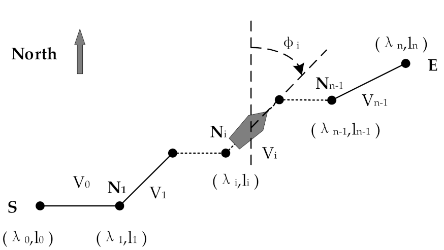
As shown in Figure 2, the route planned in this study includes a series of waypoints. Therefore, the total navigation time of the ship from the departure point to the target point can be obtained by adding the time spent on each route, as shown in Equation (1).
T t o t a l = i = 0 n 1 t i ;   t i = L i V a i
Here, T t o t a l is the total navigation time of the ship, t i is the navigation time of the ship on each route section, and V a i is the actual speed of the ship on the i th route segment. If Earth is considered as an ellipsoid, the length of any two points on the Mercator projection map can be calculated as follows [10]:
l 2 l 1 tan φ r h = ln tan π 4 + λ 2 2 1 e sin λ 2 1 + e sin λ 2 e 2 ln tan π 4 + λ 1 2 1 e sin λ 1 1 + e sin λ 1 e 2 ,
L r h = λ 2 λ 1 sec φ r h ,
where λ 1 and l 1 are the latitude and longitude coordinates of the first point, respectively, λ 2 and l 2 are the latitude and longitude coordinates of the second point, respectively, φ r h is the direction of the rhumb line, L r h is the distance between two points (in radians), and e is the eccentricity of Earth. The above formula can be applied to ships sailing along the non-isolatitude lines. However, in the case of isolatitude lines, i.e., when the ship’s heading is 90° or 270°, the following equation can be applied.
L r h = ( l 2 l 1 ) cos λ 1 .

2.2.2. Meteorological Risk

It is necessary to understand the degree of threats to the safety of ship navigation caused by weather and ocean conditions. The IMO has given out information on how the captain should choose the route to avoid the navigation risk zone under severe sea conditions [21], but it did not assess the overall risk status of the route. In this section, we comprehensively consider wind, waves, and seakeeping to assess ship navigation risks and propose a comprehensive risk calculation formula to adapt to route optimization under good and severe sea conditions.
According to the “2008 International Intact Stability Regulations” [22], the stability criterion K should satisfy Equation (5) to ensure that ships navigate safely in strong winds.
K = L q L f 1 ,
where L q represents the minimum overturning moment arm, which can be obtained from the dynamic stability curve and roll angle. L f represents the wind pressure roll arm, and its value can be obtained using Equations (6) and (7).
L f = P A f Z 1000 g Δ ,
P = C p ρ u 2 2 ,
where P represents the unit calculated wind pressure, A f represents the wind area of the ship, Z represents the height from the center of the wind area to the water surface, g represents the acceleration of gravity, Δ represents the ship displacement, C p represents the wind pressure coefficient, ρ represents the air density, and u represents the average wind speed. Based on Equations (5)–(7), the crosswind speed that the ship can withstand 10 m above the sea surface should satisfy Equation (8).
u 10 u 10 max = 40 10 Z 1 8 10 Δ L q C p A f Z ,
According to the maximum crosswind that can be withstood by the ship, a numerical expression of the risk of wind to the ship is established, as shown in Equation (9), where u c r o s s represents the lateral wind speed experienced by the ship. The risk is a gradual process. We think that when the value is greater than 0.6, it is unacceptable. When it is less than 0.6, a route with as low a risk value as possible should be chosen.
r i s k w i n d = u c r o s s u 10 max ,     i f   t h e   v a l u e   i s   l e s s   t h a n   1 1 ,                       e l s e .
Under severe weather conditions, rolling is an important factor that causes a ship to capsize [23]. Therefore, in this study, the risk value caused by waves is described according to the rolling of the ship. The encounter period between the ship and wave is shown in Equation (10).
T E = λ 1.25 λ + V cos μ ,
where λ represents the wavelength, V represents the shipping speed, and μ represents the angle between the ship’s motion direction and wave direction.
The natural rolling period, T θ , of the ship can be calculated as follows:
T θ = 2 C B G M ,
where C represents the rolling period of the ship, B represents the width of the ship, and G M represents the height of initial stability.
According to the resonance theory of a ship in waves, the ship is in the harmonic rolling area when 0.70 < T θ / T E < 1.3 . In this area, a ship may have a large roll angle, threatening its safety [23]. Therefore, we have established a numerical expression for the risk of waves to ships as follows.
r i s k w a v e = T θ T E ,                     i f   0 T θ T E < 1 2 T θ T E ,           i f   1 T θ T E < 2 0 ,                           T θ T E 2 .
According to Equation (12), there is an absolute risk when r i s k w a v e > 0.7 , and when it is less than 0.7, the risk gradually decreases.
To study the ship’s motion state in wind and waves, seakeeping is a factor that must be considered. There are many factors that affect seakeeping, such as the ship’s roll, pitch, heave, the probability of the green water on deck, the probability of slamming occurrence, and bow vertical acceleration, etc. In this study, seakeeping is determined by the following three factors: the amplitude of the pitch motion, the probability of slamming occurrence, and the probability of green water on deck. The limit values of the pitch amplitude are based on the NATO STANAG, Standardization Agreement, 4154 criteria, slamming probability and green water on deck probability comply with the NORDFORSK 1987 criteria [24,25], as detailed in Table 1.
The ship’s risk obtained by considering seakeeping is determined according to Equation (13) [26]:
r i s k s e a k e e p i n g = 1 max 0 ; 1 R M S p R M S p l 1 P s p P s p l 1 P w d P w d l ,
where R M S p is the root mean square (RMS) of the pitch motion amplitude, P s p is the probability of occurrence of slamming, P w d is the probability of water on deck.
Based on the ship Response Amplitude Operator, the RMS of the pitch motion amplitude is determined according to the following equation [27,28]:
R M S p = 0 H 5 ω e 2 S ς ω e ,
where H 5 is the speed-dependent pitch motion transfer function, S ς is the wave spectrum, ω e = ω ω 2 ψ is the encounter wave frequency that satisfies the Doppler shift equation, depending on the absolute wave frequency, ω, and the factor ψ = U cos μ / g , where the vessel speed is denoted by U and μ denotes the heading angle [29].
P s p = e v c r 2 2 C s 2 m 2 , r + d 2 2 C s 2 m 0 , r ,
where v c r = 0.093 g L is the threshold velocity, C s is the swell up coefficient, and d is the ship draught at the forward perpendicular. m 0 , r and m 2 , r denote the zero-order and second-order spectral moments of the ship’s relative motion as regards the sea surface [29].
P w d = e f b 2 2 C s 2 m 0 , r ,
where f b is the freeboard at the ship forward perpendicular.
Based on the above analysis, we established the comprehensive risk of the ship being disturbed by winds and waves in the i th route segment as follows:
r i s k i = a 1 r i s k w i n d i + a 2 r i s k w a v e i + a 3 r i s k s e a k e e p i n g i ,         j = 1 3 a j = 1 ,
Because the navigation risk is a gradual process, when a i = 1 / 3 , we believe that when the risk value is greater than 0.6, the route will be discarded. When the route value is less than 0.6, although the route is acceptable, it is still better to keep the risk value is as small as possible. The risk distribution of the entire route is
r i s k = r i s k 0 , r i s k 1 , , r i s k n 2 , r i s k n 1 .
Therefore, the total risk of a route is
R I S K = max r i s k .

2.2.3. Fuel Consumption

The total fuel consumption associated with each ship route can be obtained by adding the fuel consumption in multiple route sections. The total fuel consumption of a ship can be given as follows:
f f u e l = i = 1 m 1 ( Q t i t i ) .
The fuel consumption of a ship during navigation is related to many factors such as the main engine structure, ship type structure, loading capacity, sailing speed, fuel type, and sea conditions. The best way to develop a reliable speed–consumption function is by collecting real data about the speed and the corresponding consumption [30]. The speed–consumption function is described as an exponential function, with vessel design as a constant and speed as a variable in the exponent. In this paper, Euler’s number, e, was taken as the basis to simplify later calculation. The ship’s fuel consumption per unit time can be represented as follows:
Q t i = a e b v ,
where a and b are parameters calculated for each vessel by exponential regression. The total fuel consumption of the ship can be approximated by Equations (20) and (21).

2.3. Ship Speed Loss

When a ship is sailing, winds and waves will cause additional resistance. The actual speed of the ship under winds and waves will be lower than the speed in still water when keeping the ship’s propulsion power constant [31]. The speed loss of the ship will affect the navigation time and fuel consumption and considerably affect the results of the ship’s multicriteria route planning. Therefore, speed loss is a factor that must be considered during route planning.
The following methods are mainly used to estimate the ship’s speed loss. The first method is theoretical derivation calculation, based on which the actual speed of the ship can be estimated from the perspective of system energy conservation. However, this method is cumbersome and difficult to calculate. The second method is the test method, which uses equipment, such as pools and wind tunnels, to simulate the ship for determining the speed loss. However, the overall applicability of this method is poor. The third method is an experimental method, wherein a large amount of actual observation data is used. After statistical analysis, an empirical formula is obtained for estimating the stall. Because the third method is conducive for the introduction of the algorithm presented in this study, the calculation formula of ship speed loss proposed by Feng was used here [32].
V a = V 0 1.08 h 0.126 q h + 2.77 10 3 F cos α 1 2.33 10 7 D V 0 .
where V a is the actual speed of the ship under winds and waves, V 0 is the hydrostatic speed of the ship, F is the wind speed, D is the actual displacement of the ship, h is the significant wave height, q is the relative angle between the ship’s heading and wave direction, and α is the relative angle between the ship’s heading and wind direction.
According to the above analysis, when the ship sails in rough weather, the ship will have slamming occurrence and the green water on the deck. In order to ensure the safety of navigation, the captain will take the initiative to reduce the speed of the ship. Therefore, seakeeping must be considered to calculate the maximum speed allowed in wind and waves. In this study, when the maximum speed is exceeded, the probability of the route being selected decreases. The maximum allowable speed is determined as follows [10].
V c = exp 0.13 μ ( q ) h 1.6 + r ( q ) ,
where μ ( q ) = 12.0 + 1.4 10 4 q 2.3 , r ( q ) = 7.0 + 4.0 10 4 q 2.3 .

2.4. Population Model

The population of multicriteria PSO–GA comprises multiple individuals, and each individual is represented by a series of latitude and longitude coordinates. In Equation (19), a shipping route is represented, where X i is a two-dimensional vector containing longitude and latitude values.
X = X 0 , X 1 , X i , X n 1 , X n .
Each route can be generated in a limited search area based on the reference route. The reference route is the high-frequency route of the ship in previous voyage missions. The limited search area is the area expanded on both sides of the reference route based on the historical route characteristics of the ship. As shown in Figure 3, S and E are the starting and ending points, respectively, the reference route is the great circle route between these two points, and the area enclosed by the dash-dotted line is the search area of the ship waypoint. The upper boundary of the search area is U B , whereas the lower boundary is L B , which are represented by Equations (25) and (26), respectively.
U B = U p 0 U p i U p n ,
L B = L o w 0 L o w i L o w n ,
Here, U p i and L o w i represent the position coordinates of the upper boundary point and the lower boundary point, respectively. Individuals are randomly generated according to a uniform distribution to make the initial population evenly distributed in the entire solution space and increase the diversity of the initial population according to Equation (27). After multiple generations, the initial population is obtained.
X = r a n d U B L B + L B .

2.5. Particle Swarm Optimization and Genetic Algorithm

PSO and GA are intelligent optimization algorithms developed recently and are widely used in path planning. The PSO algorithm is a random search algorithm based on group cooperation [33]. In PSO, the particle updates itself by tracking two “extremums,” among which the first is called the individual optimal solution and the second is called the global optimal solution. PSO updates the position through Equations (28) and (29).
v i d k + 1 = ω v i d k + c 1 r a n d p p B e s t x i d k + c 2 r a n d p g B e s t x i d k ,
x i d k + 1 = x i d k + v i d k + 1 ,       i = 1 , 2 , , m ;   d = 1 , 2 , , D ,
where v i d k is the particle velocity of the d th dimension of the m th particle in the k th iteration and x i d k is the particle position of the d th dimension of the m th particle in the k th iteration. ω , c 1 , and c 2 are the coefficients, and rand is a uniform random number in the range of 0 , 1 .
GA is an optimization method developed based on Darwin’s theory of natural selection [34]. When implementing GA, each individual is given a fitness level, which is the standard for measuring the quality of the individual. Then, the population is subjected to the selection, crossover, and mutation operations for obtaining a new population. Iterations are performed until the desired result is obtained.

2.6. Multicriteria Route Planning Algorithm

PSO and GA obtain good results when solving single-criteria problems but not when solving multicriteria problems. Therefore, this study combines PSO with GA and proposes multicriteria PSO–GA to solve the problem of ship route planning. The proposed algorithm mainly combines the particle cooperative operation associated with PSO, crossover operation, mutation operation, and multigroup elite selection operation in GA and improves the distribution of the Pareto solution set [34]. The flow chart of the algorithm is shown in Figure 4.
The algorithm flow will be analyzed in detail below to introduce the operation steps in the algorithm more clearly.

2.6.1. Particle Cooperative Operation

The particles in the population constantly update their positions through information exchange according to the individual and global optimal solutions. At the beginning of the iteration, the ω in Equation (28) must be large to increase the diversity of the population. As the number of iterations increases, the solution tends to become optimal. ω is gradually reduced to improve the convergence speed of the algorithm. Therefore, the speed update is determined according to Equation (30), whereas the position update is determined according to Equation (29), where M a x G e n is the maximum number of iterations. The updated speed will be lower than M a x V . Further, the route through land will be regenerated.
v i d k + 1 = 1 0.4 M a x G e n i v i d k + c 1 r a n d p p B e s t x i d k + c 2 r a n d p g B e s t x i d k .

2.6.2. Crossover Operation

In this study, the arithmetic crossover method is used to generate two new individuals from the linear combination of two individuals. By assuming that the two individuals are X 1 g and X 2 g , the calculation method of the new individual after the crossover operation is as follows:
X 1 g + 1 = X 1 g + α ( X 2 g X 1 g ) X 2 g + 1 = X 2 g + α ( X 1 g X 2 g ) ,
where α is a vector parameter with the same dimension as the individual and is a random number in the 0 , 1 interval. When the route after the crossover operation passes over land, the crossover operation must be repeated until the required route is obtained or the set number of repetitions is reached.

2.6.3. Mutation Operation

This study uses the reference route as the mean value to perform a single-point Gaussian mutation to improve the local search capability of the algorithm and search for the optimal route near the reference route. The Gaussian distribution can be determined as follows:
f x = 1 2 π σ e x μ 2 2 σ 2 ,
where μ is the coordinate value of the mutation position. The variable generated according to the Gaussian distribution has a 99.73% probability of falling in the interval μ 3 σ , μ + 3 σ . Therefore, σ can be determined as follows:
σ = U B i X i 3 .

2.6.4. Multigroup Elite Selection Operation

This study comprehensively processes the original population, the population after particle coordination, and the population after crossover and mutation to improve the quality of the global optimal solution. The three populations are merged to perform nondominated sorting, and the individual in the front after sorting is considered to be the new individual of the next generation. Domination and nondomination can be given as follows [34]:
u = F p = m i n f 1 p , f 2 p , , f n 0 p ,
u = F q = m i n f 1 q , f 2 q , , f n 0 q ,
f f i 1 , , n 0 , u i u i i 1 , , n 0 , u i < u i ,
where p and q are the decision variable vectors and the position information of the two particles is represented in the algorithm. u and u are the optimization target vectors of the two particles p and q , respectively. Because there are three optimization targets in this study, n = 3 . If the performance vectors u and u satisfy Equation (36), then particle p dominates q . If a particle neither dominates nor is dominated by other particles, the particle is called a nondominated solution. The set of all particles that satisfy the nondominated solution is called a nondominated solution set.
The crowding distance between the particles at each domination level can be defined as follows to further evaluate the performance of the particles in each domination level.
C r o w d m = j = 1 n 0 f j m + 1 f j m 1 f j M a x f j M i n ,     m = 2 , 3 , , N 1 ,
where C r o w d m is the crowded distance of the m th particle, f j is the j th objective function value, f j M a x and f j M i n are the maximum and minimum values of the j th optimization target, respectively, N is the number of particles at the same dominance level, and the crowding distance for edge particles is set to infinity.
Finally, after completing the improvement of the Pareto solution set in Section 2.6.5, a particle is randomly selected as the global optimal particle from among the particles with the highest dominating level and a degree of crowding not equal to infinity. Moreover, in each iteration, the dominant status of individuals in the population will be calculated according to Equation (36), and the population will be sorted according to the dominant level and crowding degree. Individuals with higher dominance levels will be preferentially selected to the next generation, the higher the dominance level of an individual, the closer it will be to the Pareto optimal frontier. After many iterations, individuals in the population will continue to move closer to the Pareto optimal frontier [34].

2.6.5. Improved Pareto Solution Set Distribution

In the Pareto optimal solution set obtained in Section 2.6.4, there may be cases in which multiple solutions are clustered in adjacent areas. This study will use the following steps to improve the Pareto solution distribution generated in Section 2.6.4 to make the Pareto solution set more evenly distributed in the entire solution space and avoid local convergence of the algorithm.
(1) Sort the individuals in the solution set with the highest dominance level according to the navigation risk value from small to large.
(2) Calculate the Euclidean distance, d i s i , between the nondominated solution i and the nondominated solution i + 1 in the target space. Here, f i j represents the j th objective function value of the i th nondominated solution.
d i s i = j = 1 n f i j f i + 1 j 2 ,
(3) Determine whether d i s i is less than the specified value d i s _ s e t , which is determined according to Equation (39), where n u m represents the number of nondominated solutions. If d i s i 1 < d i s _ s e t and d i s i < d i s _ s e t , delete the nondominated solution i and calculate the Euclidean distance between the nondominated solution i 1 and the nondominated solution i + 1 and assign it to d i s i 1 .
d i s _ s e t = i = 1 n u m 1 d i s i n 1 ,
(4) Determine whether the number of nondominated solutions exceeds the set value S e t N u m . If yes, move to step 5; otherwise, skip to step 6.
(5) Delete p = n u m S e t N u m nondominated solutions in the crowded area to simplify the nondominated solutions in the crowded area. The flowchart is shown in Figure 5.
d i s = d i s 1 , d i s 2 , , d i s n u m 2 , d i s n u m 1 .
(6) Return an improved set of Pareto solutions.

2.6.6. Recommended Routes

According to the Pareto frontier and Pareto solution set obtained using the proposed algorithm, the recommended route can be given as follows:
Z = min j = 1 n a j c i j y j 2 1 2 ,       j = 1 n a j = 1 ,       ( i = 1 , 2 , , M ) ,
where c i j is the normalized value of the j th objective function of the i th particle, y j is the normalized value of the expected objective function, which, respectively, indicate the navigation time, fuel consumption, and acceptable navigation risk set by the shipping company or captain before the start of the navigation mission. M is the number of particles in the Pareto solution set, and Z is the recommended route in which the conditions given on the right side of the equation are satisfied.

3. Results

3.1. Algorithm Parameter Setting

The experimental ship in this study was an S-175 container ship. The ship parameters are shown in Table 2.
The sailing area expands in both the directions along the angle bisector of the reference route. In experiment one and experiment two, the extension was 8 degrees in two directions, respectively. Meteorological data comes from the public database of the European Center for Mid-range Weather Forecast. Some ship speed and fuel consumption data used for curve fitting are shown in Table 3. In Equation (21), a = 0.1255 (95% confidence interval: (0.1171, 0.1339)), b = 0.2444 (95% confidence interval: (0.2395, 0.2493)). Root mean squared error (RMSE): 0.02781. Coefficient of determination (R-square): 0.9995. The parameters of the multicriteria algorithm are presented in Table 4.
In this table, G e n represents the number of algorithm iterations, P o P u represents the number of populations, c 1 and c 2 represent the parameters in PSO, M u represents the uniform mutation probability, C r represents the crossover probability, S e t N u m represents the specified maximum number of nondominated solutions, and M a x V represents the maximum velocity of the particle swarm. For Equation (41), in the three experiments, the weight coefficients a j of risk, fuel consumption, and time are set to 0.4, 0.3, and 0.3, respectively. This study establishes a visual simulation interface for the convenience of ship route optimization, as shown in Figure 6.

3.2. Experimental Results and Analysis

The multicriteria ship route of the S-175 container ship was optimized according to the algorithm parameters set in the previous subsection. This study included three experiments. The first was to plan routes in sea under good weather conditions, the second was to plan routes in sea under severe weather conditions, and the third was to plan routes under complex offshore conditions. In Experiment one and Experiment two, the number of route segments was set to 7, and the number of route segments in Experiment three was set to 10.

3.2.1. Good Weather Conditions

The starting and ending ports of the ship are St. John’s (47 N, 52 W) and Porto (41 N, 9 W), respectively. According to the weather forecast, from 1 to 7 July 2019, the ships sailing along the great circle route will not encounter strong winds and waves. Under this condition, the great circle route between the two ports is set as the reference route. We conducted 20 repeated experiments for this sea state and got the average navigation time of the recommended route to be 135.850 and the variance to be 0.942. The average risk was 0.239, and the variance was 2.41 × 10⁻⁵. The average fuel consumption was 490.533, and the variance was 48.703. A group of experiments were then selected for a detailed description.
After algorithm optimization, the Pareto optimal solution set of the multicriteria route is shown in Figure 7a. The Pareto optimal frontier solution is shown in Figure 7b. According to the route position information in Pareto solution collection, routes with the minimum navigation time, risk, and fuel consumption were obtained. The expected navigation time was set to 135 h, the navigation risk was set to 0.24, and the fuel consumption was set to 485 tons. According to the above-expected values and Equation (41), the recommended route was obtained, which is a compromise route obtained by balancing the three objectives. This route not only ensures that the navigation risk is within an acceptable range, but also reduces the navigation time and fuel consumption as much as possible. The schematic of the above four routes and the great circle route is shown in Figure 7c. The recommended route is shown in Figure 7d.
According to Table 5 and Figure 7, the minimum-time route and the minimum-fuel-consumption route basically coincide with the great circle route, and the voyage difference was only 4.5 and 9.52 nmi respectively, indicating that the algorithm has better route search performance. The minimum-time route, the safest route, and the minimum-fuel-consumption route are calculated by the Pareto solution set according to a single criterion. In the recommended route, these three factors are integrated to obtain a compromised and improved ship route. Further, the captain can obtain another recommended route according to the different expected objective function values. When sailing on the recommended route, the position of the ship at four different navigation times is shown in Figure 8. Under good sea conditions, the ship can sail along the recommended route with low navigation risk, fuel consumption, and navigation time.

3.2.2. Severe Weather Conditions

A multicriteria ship route planning was performed for severe weather conditions in the ship sailing area to prove the effectiveness of the algorithm presented in this study. The starting and ending ports of the ship were St. John’s (47 N, 52 W) and Porto (41 N, 9 W), respectively. According to weather forecasts, from 22 to 29 July 2019, if the ship sailed along the rhumb line, it would encounter strong winds and waves. Under such sea conditions, the rhumb line between the two ports is set as the reference route. We conducted 20 repeated experiments for this sea state and got the average navigation time of the recommended route to be 157.170 and the variance to be 0.421. The average risk was 0.416, and the variance was 2.06 × 10⁻⁴. The average fuel consumption was 437.988, and the variance was 33.739. A group of experiments were then selected for a detailed description.
After algorithm optimization, the Pareto optimal solution set of the weather route is shown in Figure 9a. The Pareto optimal frontier solution is presented in Figure 9b. According to the route position information in the Pareto solution, routes with the minimum navigation time, safety risk, and fuel consumption can be obtained. The expected navigation time was set to 152 h, the navigation risk was set to 0.42, and the fuel consumption was set to 430 tons. The five optimized routes are shown in Figure 9c. The recommended route is shown in Figure 9d, and the specific data of the optimized route are presented in Table 6.
According to Table 6 and Figure 9, when the ship sails along the great circle route, the voyage was reduced by 159.37 and 208.13 nmi than the minimum navigation time route and recommended route, respectively. However, the navigation time was only reduced by 1.118 and 3.083 h, respectively. Thus, when the ship is sailing along the great circle route, large wind waves cause serious speed loss to the ship and the ship is exposed to great risks. Therefore, sailing along the great circle route is not suitable. According to Equation (41) and the above-mentioned expected objective function value, a compromise route with an objective function value close to the expected value was selected in the Pareto solution set. When sailing according to the recommended route, the position of the ship at four different navigation times is shown in Figure 10. Under severe sea conditions, the ship could sail along the recommended route with low navigation risk, fuel consumption, and navigation time.

3.2.3. Complex Offshore Conditions

Multicriteria ship route planning was performed in the waters near the Cape of Good Hope to verify the effectiveness of the algorithm for route planning near coastal waters. The starting position of the ship was (23 S, 6 E), and the destination position was (26 S, 42 E). According to the weather forecast, from 1st to 7th March 2019, the ships sailing along the reference route will encounter heavy winds and waves. We conducted 20 repeated experiments for this sea state and got the average navigation time of the recommended route to be 183.668 and the variance to be 2.725. The average risk was 0.404, and the variance was 4.05 × 10⁻⁵. The average fuel consumption was 526.396, and the variance was 29.624. A group of experiments were then selected for a detailed description.
In this sea state, the Pareto optimal solution set of the ship route after algorithm optimization is shown in Figure 11a. The Pareto optimal frontier solution is shown in Figure 11b. According to the route position information in the Pareto solution set, the smallest-sailing-time route, the least-risk route, and the least-fuel-consumption route can be separately calculated. The expected navigation time was set to 180 h, the navigation risk was set to 0.4, and the fuel consumption was set to 510 tons for obtaining the recommended route. The four routes are presented in Figure 11c. The recommended route is shown in Figure 11d, and specific data related to the four optimized routes are shown in Table 7.
According to Table 7 and Figure 11, routes satisfying different criteria under comprehensive offshore sea conditions can be obtained after algorithm optimization. The recommended route is based on the expected objective function value. According to Equation (41), a recommended route close to the expected target value was selected in the Pareto optimal solution set. Compared with the minimum-time route, the recommended route had 0.01 higher navigation risk and 0.192 h longer navigation time, but it saved 0.483 tons of fuel. The position of the ship when sailing on the recommended route at four different navigation times is shown in Figure 12. Under complex sea conditions, it was possible to sail along the recommended route with low navigation risk, fuel consumption, and navigation time.

4. Discussion

According to the characteristics of ship navigation, this study establishes a multicriteria route planning framework for ships comprising optimization criteria, ship speed analysis, model construction, multicriteria algorithms, route evaluation, and route selection. There are three criteria for ship route optimization: minimum navigation time, minimum navigation risk, and minimum fuel consumption. For navigation risk, this study proposes a comprehensive route risk assessment model that considers wind, waves, and seakeeping. Regarding fuel consumption, this study established a mathematical model of ship fuel consumption through fitting methods. Based on this framework, this study proposes a ship multicriteria route planning method using the improved PSO–GA. The proposed algorithm not only has the fast convergence of the particle swarm algorithm but also improves the diversity of solutions by applying the crossover operation, selection operation, and multigroup elite selection operation of the genetic algorithm and improving the Pareto optimal frontier distribution. By solving the route planning algorithm, the routes with the minimum navigation time, fuel consumption, and navigation risk as well as the recommended route can be obtained. In addition, the captain can customize the appropriate route according to the route solution set to ensure that the ship can sail efficiently, safely, and economically. We conduct experiments for three different situations to verify the performance of the algorithm. According to the experimental results, the recommended route can be obtained by integrating the three aforementioned indicators, based on which the area with severe winds and waves can be avoided and minimum navigation time and fuel consumption can be realized. Therefore, the ship multicriteria route planning algorithm proposed in this study is feasible and effective.
Although this study has established a multicriteria route planning algorithm for ships, there are still shortcomings, which must be improved and perfected, mainly as follows.
  • Risk assessment module: In this study, only the impact of winds, waves, and seakeeping on the ship is considered for risk assessment, whereas visibility and the impact of other ships at sea on the ship are ignored. Future studies will consider more ship risk factors.
  • Recommended route strategy: In this study, the recommended route can be accurately determined based on the three expected target values. However, it is difficult to determine the target value under the unknown conditions associated with the historical route.

Author Contributions

Conceptualization, W.Z. and H.W.; methodology, W.Z.; software, W.Z.; validation, W.Z., Y.W., Z.Z. and H.W.; formal analysis, W.Z.; investigation, W.Z.; resources, W.Z.; data curation, Y.W. and Z.Z.; writing—original draft preparation, W.Z.; writing—review and editing, W.Z.; visualization, W.Z.; supervision, H.W.; project administration, H.W.; funding acquisition, H.W. All authors have read and agreed to the published version of the manuscript.

Funding

This study was funded by the Russian Foundation for Basic Research (RFBR) (no. 20-07-00531).

Institutional Review Board Statement

Not applicable.

Informed Consent Statement

Not applicable.

Data Availability Statement

Not applicable.

Acknowledgments

The authors are grateful to the anonymous reviewers for their valuable comments and suggestions that helped improve the quality of this manuscript.

Conflicts of Interest

The authors declare no conflict of interest.

References

  1. Chircop, A. The IMO Initial Strategy for the Reduction of GHGs from International Shipping: A Commentray. Int. J. Mar. Coast. Law 2019, 34, 482–512. [Google Scholar] [CrossRef]
  2. Wang, H.; Mao, W.; Erilksson, L. Efficiency of a Voluntary Speed Reduction Algorithm for a Ship’s Great Circle Sailing. Transnav. Int. J. Mar. Navig. Saf. Sea Transp. 2020, 14, 301–308. [Google Scholar] [CrossRef]
  3. James, R.W. Application of wave forecasts to marine navigation. Comp. Biochem. Physiol. A Comp. Physiol. 1957, 43, 195–205. [Google Scholar]
  4. Hagiwara, H.; Spans, J.A. Practical weather routing of sail-assisted motor vessels. J. Navig. 1987, 40, 96–119. [Google Scholar] [CrossRef]
  5. Lin, Y.H.; Fang, M.C.; Yeung, R.W. The optimization of ship weather-routing algorithm based on the composite influence of multi-dynamic elements. Appl. Ocean Res. 2013, 43, 184–194. [Google Scholar] [CrossRef]
  6. Smierzchalski, R.; Szlapczynska, J. Adopted isochrone method improving ship safety in weather routing with evolutionary approach. Int. J. Reliab. Qual. Saf. Eng. 2007, 14, 635–645. [Google Scholar]
  7. Shao, W.; Zhou, P.; Thong, S.K. Development of a novel forward dynamic programming method for weather routing. J. Mar. Sci. Technol. 2012, 17, 239–251. [Google Scholar] [CrossRef] [Green Version]
  8. Sen, D.; Padhy, C.P. An approach for development of a ship routing algorithm for application in the North Indian Ocean region. Appl. Ocean Res. 2015, 50, 173–191. [Google Scholar] [CrossRef]
  9. Mannarini, G.; Pinardi, N.; Coppini, G.; Oddo, P.; Iafrati, A. VISIR-I: Small vessels—Least-time nautical routes using wave forecasts. Geosci. Model Dev. Discuss. 2016, 8, 7911–7981. [Google Scholar] [CrossRef] [Green Version]
  10. Wang, H.B.; Li, X.G.; Li, P.F.; Veremey, E.I.; Sotnikova, M.V. Application of Real-Coded Genetic Algorithm in Ship Weather Routing. J. Navig. 2018, 71, 989–1010. [Google Scholar] [CrossRef]
  11. Chuang, T.N.; Lin, C.T.; Kung, J.Y.; Lin, M.D. Planning the route of container ships: A fuzzy genetic approach. Expert Syst. Appl. 2010, 37, 1948–1956. [Google Scholar] [CrossRef]
  12. Wang, L.P.; Zhang, Z.; Zhu, Q.D.; Ma, S. Ship Route Planning Based on Double-Cycling Genetic Algorithm Considering Ship Maneuverability Constraint. IEEE Access 2020, 8, 190746–190759. [Google Scholar] [CrossRef]
  13. Vlachos, D.S. Optimal Ship Routing Based on Wind and Wave Forecasts. Appl. Numer. Anal. Comput. Math. 2004, 1, 547–551. [Google Scholar] [CrossRef]
  14. Tsou, M.C.; Cheng, H.C. An Ant Colony Algorithm for efficient ship routing. Pol. Marit. Res. 2013, 20, 28–38. [Google Scholar] [CrossRef] [Green Version]
  15. Zhang, G.Y.; Wang, H.B.; Zhao, W.; Guan, Z.Y.; Li, P.F. Application of Improved Multi-objective Ant Colony Optimization Algorithm in Ship Weather Routing. J. Ocean Univ. China 2021, 20, 45–55. [Google Scholar] [CrossRef]
  16. Vettor, R.; Guedes Soares, C. Detection and analysis of the main routes of voluntary observing ships in the North Atlantic. J. Navig. 2015, 68, 397–410. [Google Scholar] [CrossRef] [Green Version]
  17. Vettor, R.; Guedes Soares, C. Development of a ship weather routing system. Ocean Eng. 2016, 123, 1–14. [Google Scholar] [CrossRef]
  18. He, Y.K.; Zhang, D.; Zhang, J.F.; Zhang, M.Y.; Li, T.W. Ship Route Planning Using Historical Trajectories Derived from AIS Data. Transnav. Int. J. Mar. Navig. Saf. Sea Transp. 2019, 13, 69–76. [Google Scholar] [CrossRef] [Green Version]
  19. Abd-El-Wahed, W.F.; Mousa, A.A.; El-Shorbagy, M.A. Integrating particle swarm optimization with genetic algorithms for solving nonlinear optimization problems. J. Comput. Appl. Math. 2011, 235, 1446–1453. [Google Scholar] [CrossRef]
  20. Liu, Z.; Liu, J.X.; Zhou, F.; Liu, R.W.; Xiong, N.X. A Robust GA/PSO-Hybrid Algorithm in Intelligent Shipping Route Planning Systems for Maritime Traffic Networks. J. Internet Technol. 2018, 19, 1635–1644. [Google Scholar]
  21. IMO. Revised Guidance to the Master for Avoiding Dangerous Situations in Adverse Weather and Sea Conditions: MSC.1/Circ.1228. 2007. Available online: https://wwwcdn.imo.org/localresources/en/OurWork/Safety/Documents/Stability/MSC.1-CIRC.1228.pdf (accessed on 15 January 2021).
  22. IMO. Adoption of the International Code on Intact Stability, 2008 (2008 Is Code). Available online: https://wwwcdn.imo.org/localresources/en/KnowledgeCentre/IndexofIMOResolutions/MSCResolutions/MSC.267(85).pdf (accessed on 15 January 2021).
  23. Sheng, Z.B.; Liu, Y.Z. Principles of Ships (Volume 2), 13th ed.; Shanghai Jiaotong University Press: Shanghai, China, 2017; pp. 64–166. [Google Scholar]
  24. Lewis, E.V. Principles of Naval Architecture, 2nd ed.; The Society of Naval Architects and Marine Engineers: Jersey City, NJ, USA, 1989; Volume 3. [Google Scholar]
  25. Faltinsen, O.M. Sea Loads on Ships and Offshore Structures; Cambridge University Press: Cambridge, UK, 1990. [Google Scholar]
  26. Stevens, S.C.; Parsons, M.G. Effects of Motion at Sea on Crew Performance: A Survey. Mar. Technol. SNAME News 2002, 39, 29–47. [Google Scholar] [CrossRef]
  27. Pipchenko, O.D.; Zhukov, D.S. Ship Control Optimization in Heavy Weather Conditions. In Proceedings of the 2010 11th AGA IAMU, Busan, Korea, 16–18 October 2010. [Google Scholar]
  28. Zhang, W.; Zou, Z.J. Time domain simulations of the wave-induced motions of ships in maneuvering condition. J. Mar. Sci. Technol. 2016, 21, 154–166. [Google Scholar] [CrossRef]
  29. Pennino, S.; Gaglione, S.; Innac, A.; Piscopo, V.; Scamardella, A. Development of a New Ship Adaptive Weather Routing Model Based on Seakeeping Analysis and Optimization. J. Mar. Sci. Eng. 2020, 8, 270. [Google Scholar] [CrossRef]
  30. Von Westarp, A.G. A new model for the calculation of the bunker fuel speed-consumption relation. Ocean Eng. 2020, 204, 107262. [Google Scholar] [CrossRef]
  31. Kim, M.; Hizir, O.; Turan, O.; Day, S.; Incecik, A. Estimation of added resistance and ship speed loss in a seaway. Ocean Eng. 2017, 141, 465–476. [Google Scholar] [CrossRef] [Green Version]
  32. Liu, F. Research on the problem of ship stalling in wind and waves. J. Dalian Marit. Univ. 1992, 4, 347–351. [Google Scholar]
  33. Kennedy, J.; Eberhart, R. Particle Swarm Optimization. In Proceedings of the IEEE International Conference on Neural Networks, Perth, WA, Australia, 27 November–1 December 1995; Volume 4, pp. 1942–1948. [Google Scholar]
  34. Deb, K.; Pratap, A.; Agarwal, S.; Meyarivan, T. A fast and elitist multiobjective genetic algorithm: NSGA-II. IEEE Trans. Evol. Comput. 2002, 6, 182–197. [Google Scholar] [CrossRef] [Green Version]
Figure 1. Multicriteria route planning framework.
Jmse 09 00357 g001
Figure 2. Route diagram comprising multiple waypoints.
Jmse 09 00357 g002
Figure 3. Expansion area. The great circle route is the reference route.
Jmse 09 00357 g003
Figure 4. Flow chart of the multicriteria route planning algorithm.
Jmse 09 00357 g004
Figure 5. Flow chart of step 5 for improved Pareto distribution.
Jmse 09 00357 g005
Figure 6. Multicriteria route planning simulation interface.
Jmse 09 00357 g006
Figure 7. Ship route optimization results under good sea conditions: (a) the Pareto optimal solution set of the multicriteria route; (b) the Pareto optimal frontier solution; (c) great circle route and four optimized routes; and (d) recommended routes.
Jmse 09 00357 g007
Figure 8. Position of the ship under good sea conditions at four different navigation times. (ad) show the positions of the ship with respect to the wave height map at different times.
Jmse 09 00357 g008
Figure 9. Ship route optimization results under severe conditions: (a) the Pareto optimal solution set of the multicriteria route; (b) the Pareto optimal frontier solution; (c) great circle route and four optimized routes; and (d) recommended routes.
Jmse 09 00357 g009
Figure 10. Position of the ship in severe conditions at four different navigation times. (ad) show the position of the ship with respect to the wave height map at different times.
Jmse 09 00357 g010aJmse 09 00357 g010b
Figure 11. Ship route optimization results under complex offshore conditions: (a) the Pareto optimal solution set of the multicriteria route; (b) the Pareto optimal frontier solution; (c) great circle route and four optimized routes; and (d) recommended routes.
Jmse 09 00357 g011aJmse 09 00357 g011b
Figure 12. Position of the ship under complex offshore conditions at four different navigation times. (ad) show the position of the ship with respect to the wave height map at different times.
Jmse 09 00357 g012aJmse 09 00357 g012b
Table 1. General operability limiting criteria for ships.
Root mean square of pitch amplitude ( R M S p l )1.5 degrees
Slamming probability ( P s p l )0.03 (L 100 m) or 0.01 (L 330 m)
Green water on deck probability ( P w d l )0.05
Table 2. S-175 container ship parameters.
ParameterLengthBreadthDepthDraughtDisplacementMetacentric Height
Value175 m25.4 m15.4 m9.5 m23,740 m31.022 m
Table 3. Ship speed and fuel consumption data.
Velocity (kn)1010.51111.51212.51313.51414.515
Fuel consumption (tons/hour)1.401.621.862.112.382.682.303.363.854.344.91
Table 4. Algorithm parameter values.
G e n P o P u c 1 c 2 M u C r S e t N u m M a x V
10050220.20.7400.8
Table 5. Objective function values of five routes in good sea conditions.
-Distance (nmi)Time (h)RiskFuel (tons)
Minimum-time Route1872.32134.2220.250486.112
Safest Route2166.99154.2890.209572.946
Minimum-Fuel Route1877.34134.7240.250485.937
Great Circle Route1867.82133.9190.259484.787
Recommended Route1867.85133.9190.256484.785
Table 6. Objective function values of five routes in severe conditions.
-Distance (nmi)Time (h)RiskFuel (tons)
Minimum-time Route2027.22156.7850.469437.612
Safest Route2179.30165.6770.405487.839
Minimum-fuel Route2024.04156.9220.476435.241
Great Circle Route1867.85155.7320.562366.094
Recommended Route2075.98158.8150.442458.005
Table 7. Objective function values of five routes in complex offshore conditions.
-Distance (nmi)Time (h)RiskFuel (tons)
Minimum-time Route2334.73182.5620.412526.436
Safest Route2520.17196.4350.402573.419
Minimum-fuel Route2344.30184.5690.420522.402
Recommended Route2335.18182.7540.413525.953
Publisher’s Note: MDPI stays neutral with regard to jurisdictional claims in published maps and institutional affiliations.

