Article

The One-Way FSI Method Based on RANS-FEM for the Open Water Test of a Marine Propeller at the Different Loading Conditions

1
Department of Mechanical Engineering, Babol Noshirvani University of Technology, Babol, Iran
2
Faculty of Civil Engineering, Technische Universität Dresden, 01069 Dresden, Germany
3
John von Neumann Faculty of Informatics, Obuda University, 1034 Budapest, Hungary
*
Author to whom correspondence should be addressed.
J. Mar. Sci. Eng. 2021, 9(4), 351; https://doi.org/10.3390/jmse9040351
Submission received: 26 January 2021 / Revised: 13 March 2021 / Accepted: 16 March 2021 / Published: 24 March 2021
(This article belongs to the Special Issue Fluid/Structure Interactions)

Abstract

:
This paper aims to assess a new fluid–structure interaction (FSI) coupling approach for the vp1304 propeller to predict pressure and stress distributions with a low-cost and high-precision approach with the ability of repeatability for the number of different structural sets involved, other materials, or layup methods. An outline of the present coupling approach is based on an open-access software (OpenFOAM) as a fluid solver, and Abaqus used to evaluate and predict the blade’s deformation and strength in dry condition mode, which means the added mass effects due to propeller blades vibration is neglected. Wherein the imposed pressures on the blade surfaces are extracted for all time-steps. Then, these pressures are transferred to the structural solver as a load condition. Although this coupling approach was verified formerly (wedge impact), for the case in-hand, a further verification case, open water test, was performed to evaluate the hydrodynamic part of the solution with an e = 7.5% average error. A key factor for the current coupling approach is the rotational rate interrelated between two solution domains, which should be carefully applied in each time-step. Finally, the propeller strength assessment was performed by considering the blades’ stress and strain for different load conditions.

1. Introduction

The propeller is the main part of a propulsion system by which engine power can move the marine vessels. Marine propellers work in an intense and complicated flow field and high-risk work conditions; those two aspects must be considered to design a new propeller. First, evaluating the hydrodynamic coefficients like efficiency and thrust and torque coefficient. Second, strength due to loads and manufactured material. The propeller blade strength role is essential in the cavitation phenomenon and propellers’ efficiency. In essence, the blades’ structural behavior has fully interacted with the hydrodynamic propulsion qualification, particularly propeller efficiency. There are two main approaches for hydrodynamic calculations of marine propellers. The first, the inviscid numerical methodologies, involve the lifting line method, the boundary element method (BEM) [1], and the vortex lattice method (VLM) [2]. The second is computational fluid dynamic (CFD) involving large eddy simulation (LES) [3], or Reynolds-averaged Navier–Stokes (RANS) [4,5,6]. Because marine propeller operates in a viscous flow and complex current of the wake, CFD methods are more suitable and efficient than the inviscid methods (BEM, VLM), albeit some researchers use the inviscid method for propeller simulation due to the low-cost and lower simulation power needed.
Many researchers have used the RANS method to overcome the rotating blades’ solution complexity, especially for marine propellers. Maksoud et al. [7] carried out how the propeller hub could change the propeller efficiency by using CFX. Another main factor in operational marine propeller condition is the propeller and rudder interaction, investigated by Simenson et al. [8]. Valentine [9] used the RANS equations to predict the propeller blades’ flow characteristics by considering turbulence inflow characteristics. In this paper, two main issues should be evaluated; first hydrodynamic calculations based on the RANS method. Second, structural analysis, that fluid–structure interaction must be engaged in the computational prediction approach. The nonlinear hydrodynamic load exerted on propeller blades due to the propeller’s rotational motion inducing a centrifugal force.
The majority of the fluid-structure interaction studies on marine propeller focus on the composite propeller; Das et al. [10] used a reverse-rotation propeller in a CFD analysis. Mulcahy [11] investigated a comprehensive study on the composite propellers’ hydro-elastic tailoring. In 2011, Blasques et al. [12] investigated the propeller’s hydrodynamic improvements using different laminate layups for optimal speed and fuel consumption. In 2008, Young [13] investigated marine propeller fluid-structure interaction analysis to assess the composite blade’s behavior. Also, the Tsai-Wu strength criterion is considered to evaluate the blade strength. Lee et al. [14] investigated a two-way coupling approach consisting of added mass based on the coupling between boundary element and finite element method. He et al. [15] used a hydro-elastic approach to evaluate composite propeller’s performance, especially vibration due to loads on propeller hub and the composite layup scheme shaped based on coupling CFD and FEM methods. Finally, a comprehensive study for four propellers with different concerning materials was published in 2018 by Maljaars et al. [16], consisting of RANS–FEM and BEM–FEM results versus experimental results. Hong et al. [17] developed a pre-twist approach to gentrify the propeller’s hydrodynamic characteristics using FEM/CFD-based software, ANSYS/CFX. Han et al. [18] used Star-CCM+ and Abaqus coupling approach to study the marine composite propellers; the results were reasonably close to experimental outputs. Paik et al. [19] investigated different composite propellers numerically and experimentally. In 2020, Shayanpoor et al. [20] performed an analysis by considering the CFD–FEM-based approach under the two-way coupling method on the KP458 propeller.
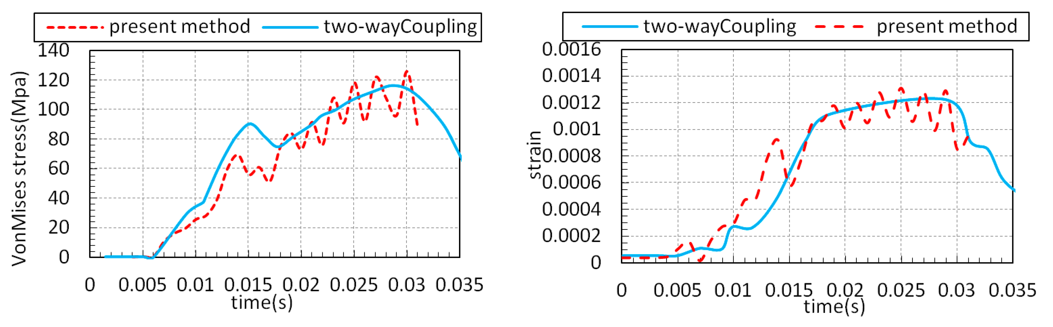
A simple FSI surrogate modeling is introduced in the present study by considering two distinct solvers, Linux-based/open access solvers (OpenFOAM) and windows-based/commercial software (Abaqus); thus, the major challenge is the coupling approach by considering the propeller’s dynamic motion. Accordingly, the pressures extracted from OpenFOAM transfer to Abaqus in each predetermined time-step, to use as structural load, the rotation rate and the number of time-steps should be first evaluated. In the following sections, for the first step, hydrodynamic solution verified with experimental tests. For the structural solution, the current FSI approach compared with the wedge impact case was verified later; the justification of using the wedge impact verification is the similarity of the two cases. For the second step, the verified numerical model performs to analyze the advance coefficients’ effect on the forces and stresses imposed on the propeller blades.

2. Materials and Methods

Fluid–structure interaction approaches are divided into monolithic and partitioned methods. In addition, partitioned methods are divided into one-way and two-way approaches. Moreover, two-way coupled is divided into strong and weak approaches [21]. From the accuracy aspect, the two-way coupling approach is more accurate than the one-way approach, especially for cases with more significant deformations and deflections. On the other hand, the one-way coupling requires less data for a single iteration per time-step. In addition, the mesh advocated for the fluid domain needless to be recalculated at each time-step. This leads the numerical solution to remain stable with unchanged mesh quality. Thus, the needed time related to the numerical solution is lower than two-way coupling, updated only after each time-step for a new iteration. Therefore, an overriding advantage of the one-way coupling approach is decreasing in the numerical solution time. Piro’s [22] compared the one-way and two-way coupling approaches (RQS-RDyn-TC) for different plate thicknesses, the discrepancies between the methods were small for thick plates; whatever the plate’s thickness becomes small, the accuracy of one-way coupling decrease. Due to the small deflection that occurred for the propeller blades in the present study, the one-way coupling method could be accurate enough.

2.1. Governing Equations of the Flow Around the Propeller

The most applicable and usable approach for simulating turbulent regimes is based on solving the Reynolds-averaged Navier–Stokes (RANS) equations. In the present study, InterDymFoam, a multiphase solver of OpenFOAM libraries, is used for hydrodynamic simulation. InterDymFoam is a proper solver based on the RANS equation by considering multi turbulence models [23] for dynamic mesh cases. The fluid is regarded as an incompressible Newtonian fluid that should inherently satisfy the mass conservation and momentum equations. The RANS equations are based on time-averaged variables decomposing the velocity, pressure fields into:
u = u ¯ + u p = p ¯ + p u ¯ = u ¯ i + v ¯ j + w ¯ k u = u i + u j + w k
u i x i = 0
( u i ) t + ( u i u j ) x j = f i 1 ρ p x i + x j [ v ( u i x j + u j x i ) + τ i j ]
x i = ( x , y , z ) represents coordinates, u i = ( u , v , w ) are the component of Reynolds-averaged velocity. ƒi denotes the body forces presented as forces per unit volume and in the present study assumed that f i = 0 . Moreover, u, ρ , and P are fluid velocity vectors, density, and pressure, respectively. The Boussinesq assumption is considered to represent the Reynolds stress for incompressible flows, which is commented below:
τ i j = υ t ( u i x j + u j x i ) 2 3 δ i j k
k = 1 2 ( ( u ¯ ) 2 + ( v ¯ ) 2 + ( w ¯ ) 2 ) ,   u = u u ¯ ,   u ¯ = 1 T 0 T ( u ( t ) u ¯ ) d t
where ν t represent the turbulence eddy viscosity, k denotes turbulent kinetic energy (TKE) per mass. In addition, δ i j surrogate as the Kronecker delta. u ¯ is time-averaged velocity, in which u ¯ and u ¯ 2 are the mean and variance velocity, respectively. A two-equation turbulence model (k-ε) is used for the present study. ε denotes the dissipation rate of energy per mass, which determines the amount of energy lost by the viscous forces in the turbulent flow that should be introduced. ( μ t ) is turbulent viscosity:
μ t = ρ C μ k 2 ε
ε = 1 2 μ ρ { u + ( u ) T } : { u + ( u ) T } ¯
To track the particles and capture the interface for the multiphase solution easily, the volume of fluid (VOF) could be a practical approach. The VOF method uses a volume fraction variable α to represent the air and water portion in each finite volume cell [24], where ρ 1 and μ 1 represent the physical properties of water, and ρ 2 and μ 2 also mean the physical properties of air, which introduces new conservation equations:
ρ = α ρ 1 + ( 1 α ) ρ 2 ,   μ = α μ 1 + ( 1 α ) μ 2 , α = 0 :   a i r α = 1 : w a t e r
The two-phase dynamic solution similar to the present case (propeller in water) is transient with a high turbulent regime that caused the solution to be inherently unstable. There were some algorithms to couple the mass conservation and momentum equations, the semi-implicit method for pressure-linked equations (SIMPLE), and the pressure implicit with the splitting of operators (PISO) that in the present study, the high-fidelity algorithm based on merging the PISO and SIMPLE called PIMPLE used.There are two important parameters, inner and outer correctors; inner corrector is the number of times the pressure is corrected, and the outer corrector is the number of times the equations are solved in each time-step. Outer corrector puts an obligation to stop the solution for each time-step apart from the solution be converged or not.

2.2. Governing the Structural Equations

Structural analysis is an essential step for one-way coupling approaches that should be performed correctly. The cantilever beam model is the initial theory to calculate the propeller blade strength introduced by Taylor [25]. This method was implemented and developed by some researchers. The method’s drawback was poor results for the points with a low thickness on the propeller’s blade compared to thicker blade’s sections near the propeller’s root. This problem continued until the introduction of shell theories developed by Cohen [26] and Conolly [27], the limitation of this method was the propellers’ geometry complexity. For instance, wide-blade or high-skew propellers could not be assessed accurately, but in recent years, the finite element method used widely by dividing into solid or shell element approaches. Many investigations are based on both approaches, but Young [13] and Blasques et al. [12] performed a study to evaluate the output results’ differences. Their investigation indicates that, although both methods are sufficient, the Shell element model needs lower computational power than the solid element method. Moreover, the solid element method has some prominency rather than a shell element model, Young [13]; this is why most FSI problems used a solid element model for the structural solver.
The deflection due to the structure’s imposing loads is the main issue [28] performed by the finite element method. This technique broadly consists of discretizing a structure into several elements that should be assembled at the end. In addition, internal stresses are in equilibrium due to the continuity of stress for interface elements. The present finite element uses the explicit method, in which a time-based approach (central difference method) is used to integrate the equations of motion. In this method, the period is considered small enough to prevent divergence [29]. The equation of motion for the structural deformation corresponding to the propeller blade fixed coordinate is introduced by Equation (9):
M s d ¨ + C s d ˙ + K s d = F S T
where M s is the mass matrix, C s belongs to damping matrix and K s represent the matrix for the structure stiffness. the variables d ¨ , d , d ˙ are the acceleration, velocity, and displacement, respectively. F S T is the summation of all loads imposed on the structure. Importantly, for the cases like a propeller, this load comprises force due to rotation, centrifugal force and moments, Coriolis force, and external load on the structure. For the case in hand, due to static analysis of the propeller and motionless blades in each time-step, the only pressure used for calculation is the fluid pressure extracted from the CFD solution. The calculation algorithm’s first step is to solve the dynamic equilibrium relation, Equation (11). The kinematic conditions solve the next iteration’s kinematic constraint in each distinct increment.
U ¨ = ( M ) 1 ( P I ) t ,   M U ¨ = P I
U ˙ ( t + Δ t 2 ) = U ˙ ( t Δ t 2 ) + ( Δ t ( t + Δ t ) + Δ t ( t ) 2 U ¨ t
U ( t + Δ t ) = U ( t ) + Δ t ( t + Δ t ) U ˙ ( t + Δ t 2 )
All of these parameters belong to nodal points, where M is the nodal mass matrix, U is nodal displacement and U ¨ is nodal acceleration. To govern net forces act on nodal points (P–I) is used, that p is the external loads imposed on the structure. This parameter is considered nodal forces. The integrated accelerations are used to calculate velocity variations; this new added velocity value from the previous middle increment determines the middle of the current increment Equation (11). then The time-integrated velocities are added to the beginning displacements’ increment to determine the final displacements’ increment, Equation (12); after estimation of the nodal displacement in time(t), the element strain increments are calculated from the strain rate, The stress components can be calculated from constitutive equations and the solution process repeated for time (t + ∆t).

2.3. Modeling and Computational Setup

2.3.1. Open Water Test Characteristic

The present study’s framework is a numerical solution related to the Potsdam propeller test case (PPTC). For this purpose, the same propellers’ geometry with the same material is accepted from the experiment cases, represented in Table 1 and Table 2, respectively [
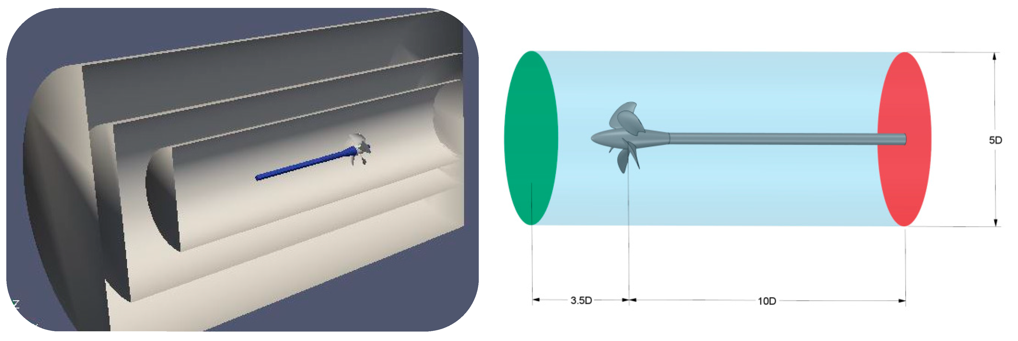
29]. The International Towing Tank Conference (ITTC) recommended that the propeller rotational speed is considered constant, but propellers’ advanced speed varies for different advance coefficients. The incident flow into the propeller is the opposite of real working conditions; propellers must be rotated in the opposite direction. We will hereafter comply with this rule to perform open water tests. The solution domain is modeled cylindrically with the following dimensions; 3.5 D forward, 10 D rearward, and 5 D in diameter, D is propeller diameter [30] (Figure 1).
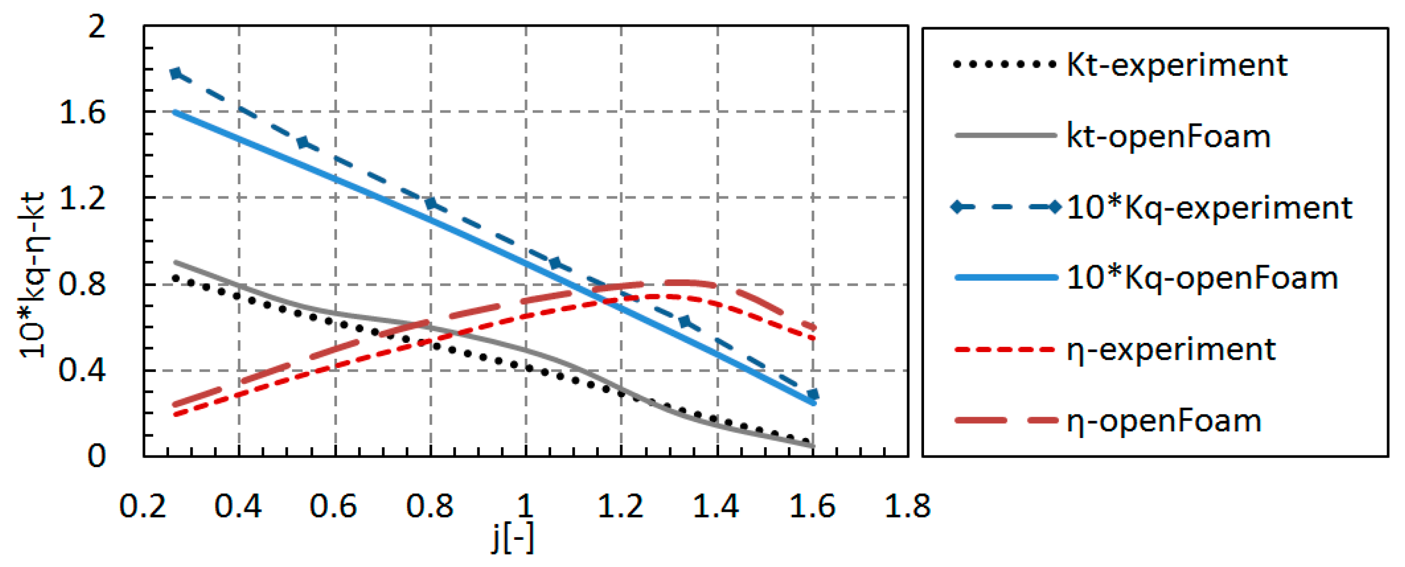
For the open water tests, The main parameters are the thrust coefficient k t , and torque coefficient k Q , represented by the dimensionless values mentioned in equation (13). The coefficients are directly related to rotational speed, n, diameter, D of the propeller, and water density, ρ . Furthermore, T represents thrust [N], Q is equal to torque [Nm], V a denote the advance speed [m/s], and η is proportional to the efficiency [-].
J = V a n D , k t = t h r u s t ρ n 2 D 4 , K q = T o r q u e ρ n 2 D 5 , η = K T J 2 π K Q

2.3.2. Applied Boundry Condition and Dynamic Motions Method

Although various boundary conditions can be devoted to, accurate results without divergence need a proper allocation of boundary conditions In the present case, the inlet and outlet boundary condition was set based on the downstream of the outlet boundary domain. For the inlet boundary condition, free-flow velocity is considered constant, dependent on advance velocity for each advance coefficient. Moreover, the inlets’ turbulence intensity is considered, I = 5%. Two main approaches could simulate the propeller’s dynamic motions, multi-reference frame (MRF) and arbitrary mesh interface (AMI), since the AMI is more practical for propeller case studies used in the present numerical solution. This method is based on the interpolation between two distinct but adjacent domains connected with an interface [30]. Two similar cylindrical domains encompass the propeller, one is static, and another one is dynamic, moves with the propeller’s rotation. Although there was no physical relationship between the two zones, the fluid and numerical calculations were transported through the interface.
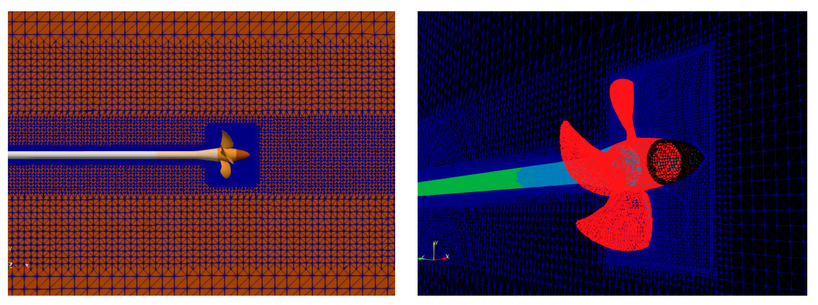
An appropriate mesh quality and structural-based domain around the propeller needs some consecutive cylinders for dividing the domain into some sub-domain. The smallest cylinder is a small grid size, and the subsequent cylinder is larger than the former cylinder. In this regard, snappyHexMesh is used as the main tool and rhinoceros’ role as an assistant tool to generate the numerical solution mesh. As shown in Figure 2, a high-quality structured mesh can be obtained by considering these techniques. A mesh independence study was established for the accuracy of the CFD solutions besides keep the computational cost.
The mesh generation framework is explained, but the mesh independence study must be performed simultaneously. The mechanism whereby the performance of griding qualified is highly dependant on the main propeller characteristics shown in Equation (12); that is how the mesh could be alleviated the computational cost without losing the accuracy. The propeller rotational speed, ω = 15 rps, and advance speed, v a = 2 m/s, the advance coefficient, J = 0.53 [-] is considered to perform the numerical solution, Table 3. The calculation for this advanced coefficient involved five different initial grid sizes, Table 4, dynamic multiphase solutions, InterDyMFoam, which comes from OpenFOAM libraries with the same underlying physics relative to InterFoam. The thrust and torque are extracted from the postprocessing tool as the initial value; then these values substitute in Equation (13); finally, the results for each simulation are gathered in Table 4; all these cases provided acceptable results. Consequently, fine (IIII) resolution leads to a reasonable prediction of thrust and torque coefficient with optimum computational cost compared with other cases.

3. Results and Discussion

3.1. CFD Validation

The numerical model tests are performed base on the advanced coefficient shown in Table 5, the same as the experimental tests [31]. As before said, the numerical investigations performed based on InterDymFoam to derive the thrusts and torques forces, then these values substitute in Equation (13) to obtain the trust coefficients, torque coefficients, and efficiency. These coefficients are calculated and compared with the experimental values; the resemblance between the present study results and the experiments is sufficient, Figure 3. Neither this numerical method nor any other methods could not achieve accurate results for low advance coefficients. That is why the error is an intrinsic part of the simulation, especially for low advance coefficients. In fact, the J = 0.266 error percentage does not account for the average error calculation. The reason is, due to severe turbulence flows around the propeller, the maximum error percentage belongs to the highest turbulent rate, J = 0.266, which caused unavoidable discrepancies. Finally, e = 7.5% is considered as the average error percentage for the present method’s efficiency.

Hydrodynamic Analysis of the vp1304 Propeller

Four advanced coefficient-related contours are illustrated in Figure 4 to show the motion of the flow’s particles around the propeller, particularly around the faces and backside. In essence, for the bigger advance coefficient, the blade’s pressure gradient decrease; this leads the propeller’s thrust and torque to be lower than the smaller advance coefficient. That is why the maximum propeller’s thrust occurred at bollard state (advance velocity = 0), and after this, it gradually decreased until it reached near zero for j = 1.6 onwards. Because the pressure and velocity are interrelated, the flow field’s evaluation for the velocity should be considered. The discrepancies between j = 0 and j = 1.23, minimum and maximum advanced coefficient, for the velocity contour are affected by the direction and disparity of the propeller’s flow. As the advanced velocity increases, the propellers’ backflow becomes more parallel with low dispersion, and the velocity is smoother around the propeller; accordingly, the hydrodynamic gradient pressure for propeller blades decreases.
For an in-depth analysis of how the propellers’ blades pressure changed through the centerline, three pressure gauges shown in Table 6 are considered on the propeller surface to record the outputs pressure. As shown in Figure 5, for p-1, near the blade root, the pressure values apart from the advance coefficient are in a closed interval. This trend is somewhat true for p-2, middle of blades, but for p-3, near the leading edge, the value for j = 0 and j = 1.266 are almost six times than j = 1.26. The increasing rate for pressure is so sensitive for the leading edge points. However, the utmost diagram trends are linear for different advanced coefficients; for j = 0.8, the pressures’ variations are not in an approximate line and have diagram extremums.
The valid question is, to what extent has the force dispersion on the propellers’ blade changed? This question is answered by following the same approach of the pressure evaluation. Upon that, ParaView, a visualization and postprocessing tool for OpenFOAM, is accomplished for force evaluation. A framework for the force solution is generated and captured each propeller blade surface and adopted normal vectors on these surfaces. After this, by multiplying the pressure with these normal vectors, the force could be extracted from the hydrodynamic solution. There is another method to capture the imposed force by adding force-Library to the OpenFOAM solver. This method’s drawback is that these codes must be added to the solver before the numerical solution started; thus, it is useless when a solved case wants to be evaluated. As shown in Figure 6, the maximum force imposed on the propeller occurred at J = 0; the smallest advance coefficient, J = 0.266, experienced the force (F = 600 N) similar to the bollard pull value (J = 0).

3.2. Fluid–Structure Interaction Validation

3.2.1. Finite-Element Method

Von Mises stress calculation is at the scope coverage of the present method by implementing the static/general solution of Abaqus solvers. Substantially the propeller’s dynamic motions are only considered in the CFD approach, and it is reasonable to suppose that the propeller is fixed for each time-step in the structural solver. As before said, the FEM solver used solid elements with three translation degrees of freedom, the displacements, and rotations (u, v, w, ϕ1, ϕ2). Moreover, weight functions (δu, δv, δW1, δw2, δw3) are approximated:
u = j = 1 n u j . ψ j ,   δ u = ψ i   φ 1 = j = 1 n w 2 j . ψ j ,   δ w 2 = ψ i v = j = 1 n v j . ψ j ,   δ v = ψ i   φ 2 = j = 1 n w 3 j . ψ j ,   δ w 3 = ψ i w = j = 1 n w j . ψ j ,   δ w 1 = ψ i
These Lagrange interpolation functions (ψi) are substituted in the differential equations’ weak form [32]. These functions are nodal parameters (x and y) in which x and y are nodal displacements. At the finite element methods based on displacement, the displacement’s manner in the element boundaries is not separated; unlike the strains, that the manner of strain is continuous only within one element. The point here is, choose between the linear or quadratic elements. Indeed, the strains have a constant value in linear elements, but in quadratic elements, the strains are nonlinear with more accurate strain or stress results than linear elements. According to Barlow [33], strains and stresses can be solved without limitation in the element, just for points, including defined nodes.

3.2.2. One-Way Coupling Approach

There are two main modes, dry and wet modes, with the critical factor of “added mass-generated effects” due to structural deformations. Dry condition considers only material/structural damping and wet condition consider added mass due to the blades’ vibration. Wet modes are computed by finite element embedding the structure in a fluid domain modeled by acoustic elements. When the propeller reaches maximum load at real state condition, blades begin to vibrate on their natural frequencies that, analysis under “wet” condition can give more accurate and reliable results, especially for large deformations. Due to the Investigation of Lee et al. [14], the difference between the results of the dry and wet conditions is not significant, especially for the case with low deformations. Thus, the one-way coupling with the dry condition used in the present study could perform accurate results. Nevertheless, the underlying physics dominant on the one-way coupling caused fluctuating trends due to large deformation and membrane forces rather than two-way approaches.
An aluminum wedge’s results are considered and verified with Agard and Pancirolis’ investigation [34] to evaluate the model’s applicability. The wedge characteristic used for the numerical solution is shown in Table 7 and Table 8; two variables were considered for the verification purpose, von Mises stress and strain. Since the maximum value for these variables occurred at the midpoint of the wedge wing, 150 mm from the wedge apex at the interior side (1 [mm] above the neutral axis), and Whatever the deformations larger, the accuracy challenge for the represented one-way approach is more dependable: thus, the method is verified under the most complicated state. In the present method by considering the wedge impact verification case, Agard [24], which was previously verified, Figure 7, the method adoption performed well for the propeller rotation. The similarity of steps and methods for the present study rather wedge impact can be reliable enough to use as a base approach of the vp1304 propeller. With this justification, this verified process can be utilized to analyze the propeller with a small but essential amended step; this involved the propeller’s rotation at each time-step for the structural solver, which is discussed further in the next sections.
In the present study, the structure is considered as a rigid body for fluid simulations that the flexural mass is neglected in rigid/quasi-static (RQS) approximation. Thus, the hydrodynamic forces and pressures are independent of the structure deformations. In Equation (15), f R ( t ) considered as the fluid force and the deformations δ R Q S extracted from this method are always smaller than the real deformations. As said in Heller and Jasper [35], a “dynamic amplification factor” must be applied due to neglecting the flexural mass to correct error predicting.
The coupling process’s first step is gathering the hydrodynamic data by performing the numerical solution for the marine propeller accomplished with InterDyMFoam akin to OpenFOAM libraries. The hydrodynamic data for a rigid body has mainly involved the point-by-point exerted pressure on the propeller’s surface, collected as an Excell file for the ease of transferring. Now the question is how the pressures should impose on the propeller in the structural solver. Two steps were needed to perform the Abaqus analysis. The first, the time-step assessment, involved the number of separate cases in the Abaqus solver must be determined based on Equation (16). The extracted pressures from the CFD solver were considered as a load condition at the FEM solver for the related designated time-steps. Each case at Abaqus was solved distinctly, and the results were recorded for the final datasheet. All these procedures are represented in the chart shown in Figure 8.
k . δ R Q S = f R ( t )
( a ) ,   ω = 2 π T   ( b ) ,   n = t T   ( c ) ,   m = 360 n
In more detail, the FEM part of the method could involve a set of data for different cases in each time step; the rotation rate is constant for all advance coefficients due to constant rotational speed (ω = 15 rps). The rotational rate is obtained at each time step by substituting the related values in Equation (15), θ = 27 ° . The number of time-steps for the two complete revolutions is C = 23 distinct cases. Although there were five tables for each advance coefficient, Table 9 is represented as a sample to show how the time-steps were selected and to what extent the propeller must rotate at a specific time to match the propeller’s position with the CFD solver. The number of cases, number of time-steps in Abaqus is selectable and can be increased to achieve smoother diagrams with lower fluctuations; also targeted reduction in the number of time-steps to achieve lower cost and time of the simulation. As shown in Table 9, the maximum stress and strain for each time-step were evaluated to engage in the final outputs.
The comprehensive question is, how do we diagnose the reliability of the one-way rather than two-way coupling or the advantages of using the one-way method? First, for the small deflections, significantly smaller than the body’s thickness, classified in the nonlinear deflections, the one-way is similar to two-way coupling results, and whatever the deflections became larger, the accuracy of the one-way approach decrease. For the case at hand, propeller deflections were classified in the range of low-deflection cases; thus, this approach could be reliable enough. Agard [24] used a parameter, the wetting equation (WQ), to classified the cases upon eigenfrequency and Young’s modulus for wedge impact studies to estimate the intrinsic error belong to one-way coupling. The one-way coupling named as an industrial approach due to:
  • Decrease the complexity of the numerical solution by dividing it into two parts;
  • Create two distinct mesh generation schemes depending on the grid dimension needed;
  • The ability to use one hydrodynamic solution for many structural sets, using different materials, thickness and different structural design;
  • Lower numerical solution cost and time rather than a two-way approach, the solution time is evaluated in the present study illustrated in Table 10;
  • High-fidelity results for the cases with low deflection;
  • One-way coupling is more useful for cases with large domain and multiphase systems like investigations on marine vessels, propellers, etc.

3.3. Structural Behavior of Propellers’ Blade

The propellers’ work conditions indicate that the blades should sufficiently withstand long work cycles without failure or permanent distortion. The initial research on the propeller’s structure and the analysis method was introduced by Taylor [36]. Since then, research on propellers’ hydroelastic started to include the deformations of the (high-skew) bronze propeller in the 1980s. The marine propeller’s design with the systematic propeller series was performed by Ekinci [37], who investigated B-series propellers using some empirical methods with different load conditions. The superiority of the present method is related to perform a quick structural calculation. Indeed, CFD and FEM are not correlating with each other, and the emphasis is put on using one hydrodynamic calculation for the several structural solvers.
Different cases could be performed for different materials involved Alloy or composite materials. A reasonable method to judge how the materials affect the propellers’ structures depends on two main structural variables, stress and strain. The discrepancy in value and the maximum or minimum occurrence positions are the most important factors in evaluating the propeller’s strength. To cast light on the mechanism whereby how the efficient case selected, the maximum von Mises stress imposed on the propeller used as a key factor to illustrate the stress distribution for each advance coefficient.
Apart from some exceptions, maximum stress occurred near the blades’ root, and whatever far away from the root, the value for stress decreased by a gentle slope. As predicted, when the propellers’ thrust reaches the maximum value, the propellers’ blade has deformed in the load vector’s direction. The highest value for strain and stress occurs at bollard pull (j = 0) due to thrust and torque values. As shown in Figure 9, in the bollard states’ (j = 0) maximum stress is about, s = 3 × 10 6 pa, but for another advanced coefficient, this value is oscillating about, s = 1 × 10 6 pa, and s = 1 × 10 6 pa.
For further explanation, Figure 10 used to evaluate the maximum strain and stress trends; maximum stress locations are different for each advance coefficient, at J = 1.23, the maximum value for stress is about, S = 5.2 Mpa, occurred at t = 0.08 s ((rev-1/(t = 0.66 s to t = 0.12 s)), this value is different for J = 0.8, maximum von Mises stress appears at t = 0.12 s (end of the rev-1). Such a different trend is valid for other advanced coefficients. The oscillation occurs for von Mises stress due to neglecting the damping and added mass effects for structural behavior. A contour-based figure, Figure 11, was constructed to show the stress for one revolution versus the advance coefficient The propeller’s design is such that the blade’s thickness near the hub is greater than the tip; as a result, the stress distribution indicates that stress concentration at the blade-hub intersection. The von Mises range is between S = 1.8 ×   10 6 pa and 2.4 ×   10 6 pa, except for t = 0.12 s, that is, S = 8.2 × 10 6 pa. The main assessment comprises how stress and strain distribute on the propeller’s blades and which blade absorbs the maximum load.

3.4. Propellers’ Structural Behavior in Rotation

Three different points were selected based on Table 6 to evaluate the blade rotation angle’s effects on stress distribution. The initial impression from Figure 12 is that the point near the blade root (P1), apart from the advance coefficient, has the greatest von Mises stress value, and the minimum value belongs to the point at the top of the blade (P3). Albeit, the diagrams’ harmony for three points is similar to each other. Consequently, a set of different graphs for each advance coefficient are used to illustrate how the stresses on the propeller blade’s surface are changed. Following the same approach, the von Mises stress versus the rotation angle is shown in Figure 13 for four different advance coefficients. Although the von Mises diagrams for all advance coefficients (J) are not harmonic (rev-1:0–360 and rev-2:360–720), the trend for the J = 0.266 distribution is more harmonic than other advance coefficients. j = 0.266 is a minimum point for the stress diagram; thus, the propeller’s structural behavior is more stable and has a minimum value because of maximum k t and k q , which are occurred at j = 0.266. Therefore, the main portion of exerted pressure on the propeller uses to generate thrust.

4. Conclusions

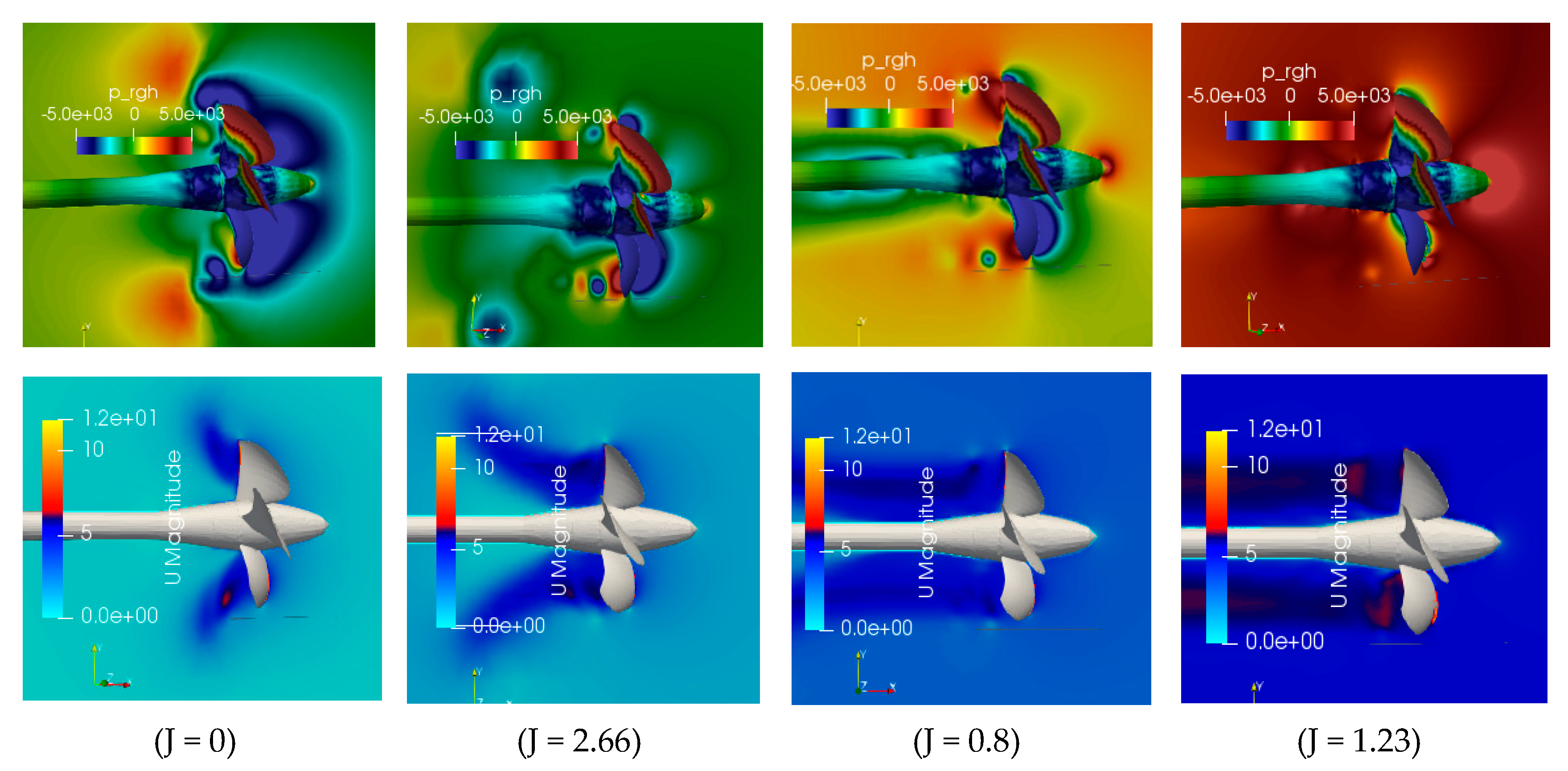
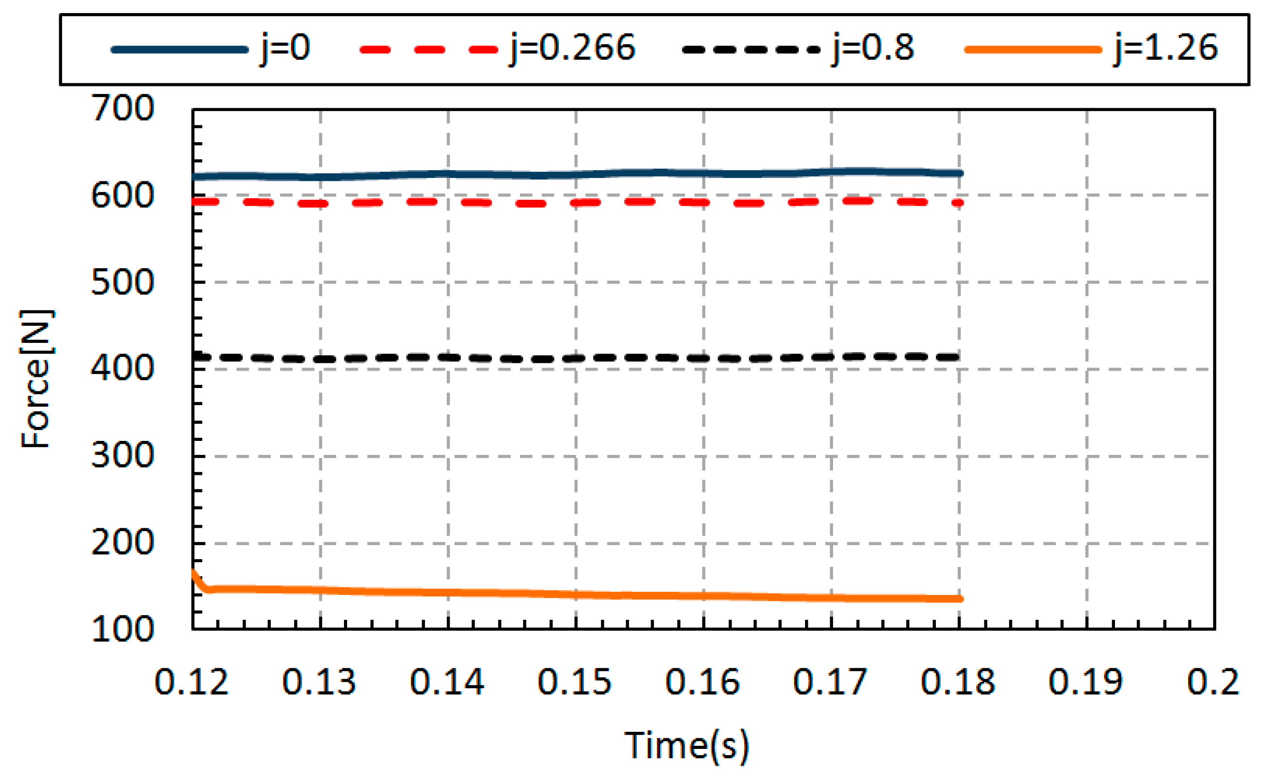
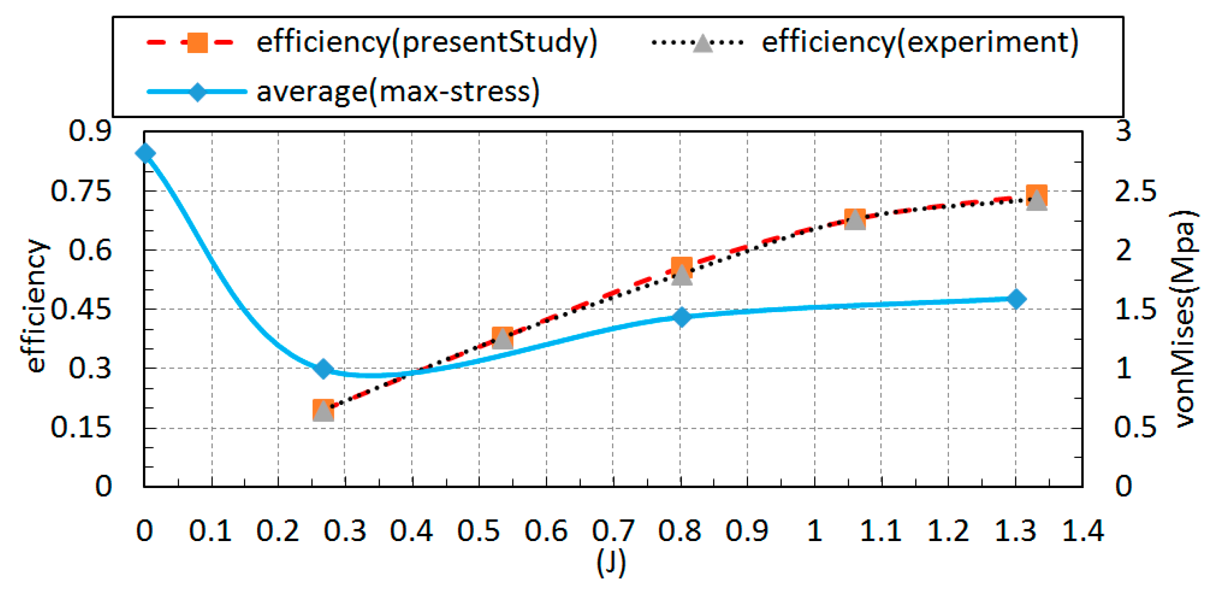
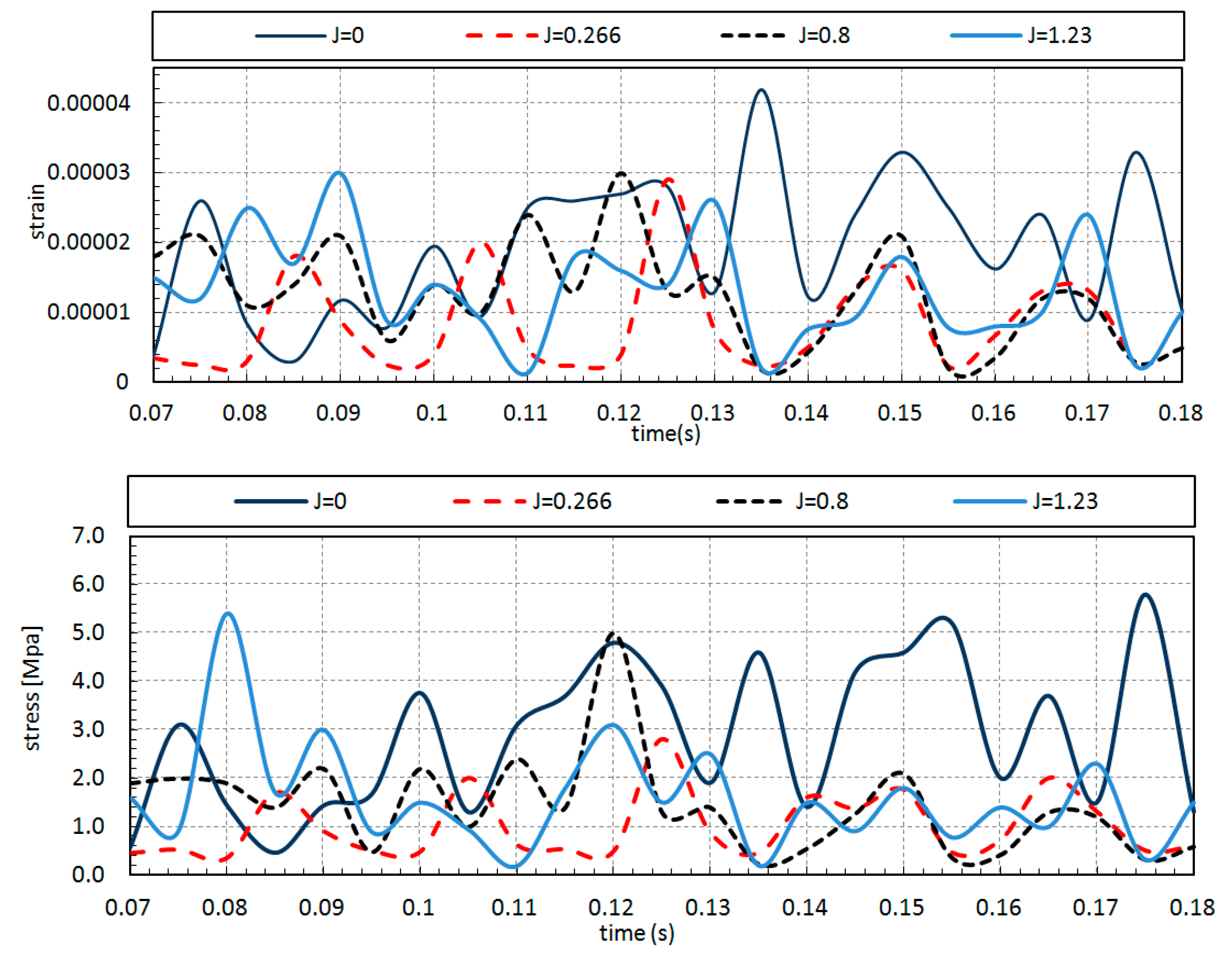
In the present study, simple surrogate modeling for rigid/quasi-static approach is used to investigate hydroelastic simulation for open water propeller test cases (PPTC); the coupling approach comprises a CFD-FEM method solved separately. In the first step, the hydrodynamic solver, InterDyMFoam, is verified with an experimental study that the average efficiency error for different advanced coefficients was about e = 7.5% for efficiency on average. For further evaluation in the hydrodynamic section, a force analysis was performed using the ParaView postprocessing toolkit for each advanced coefficient; also, pressure and velocity contours were demonstrated versus different advance coefficients.
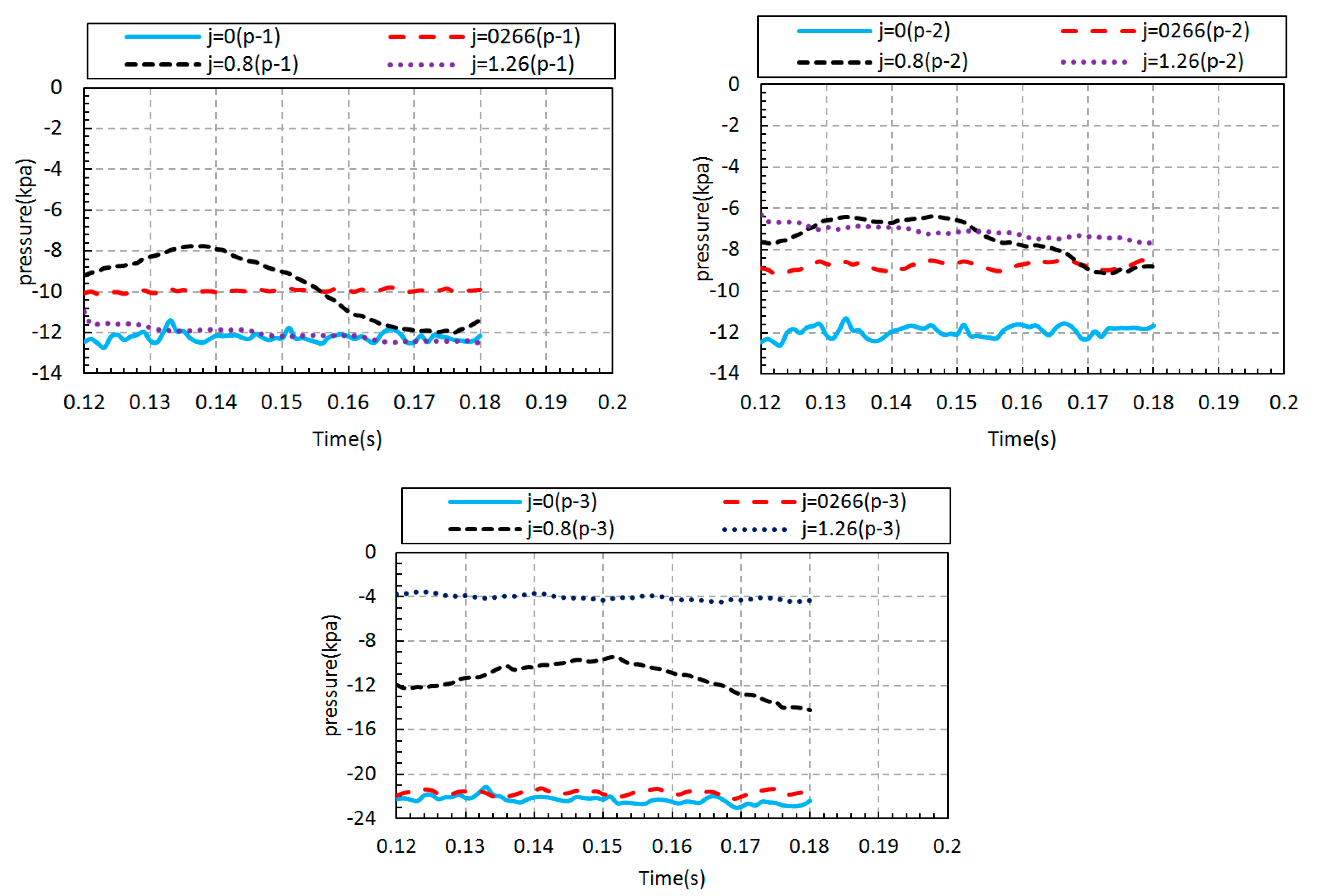
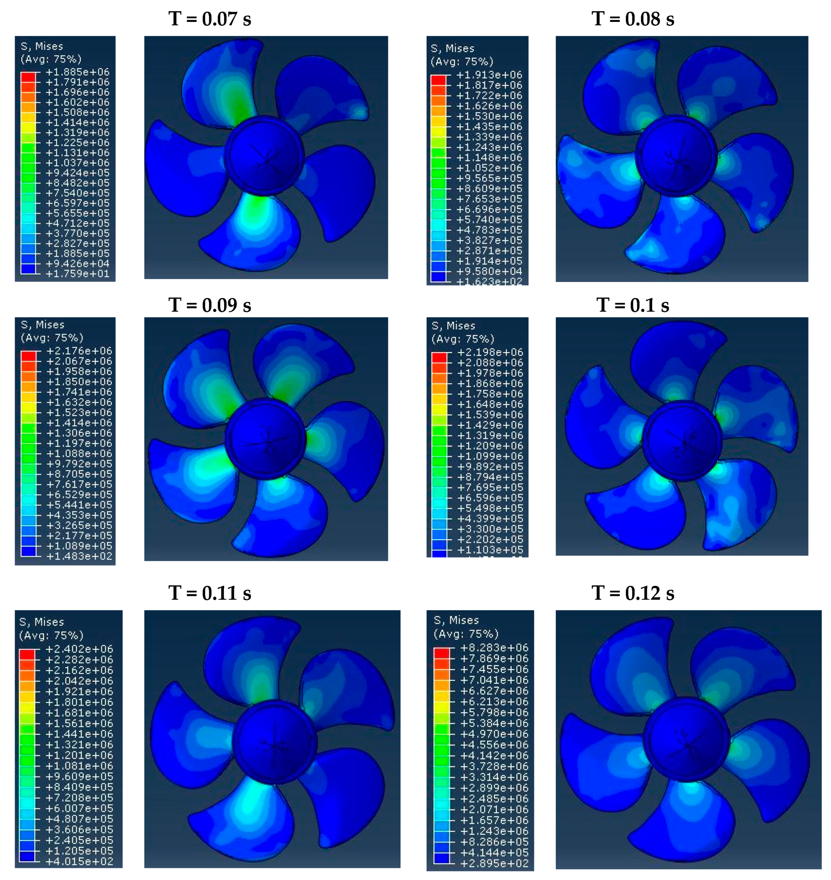
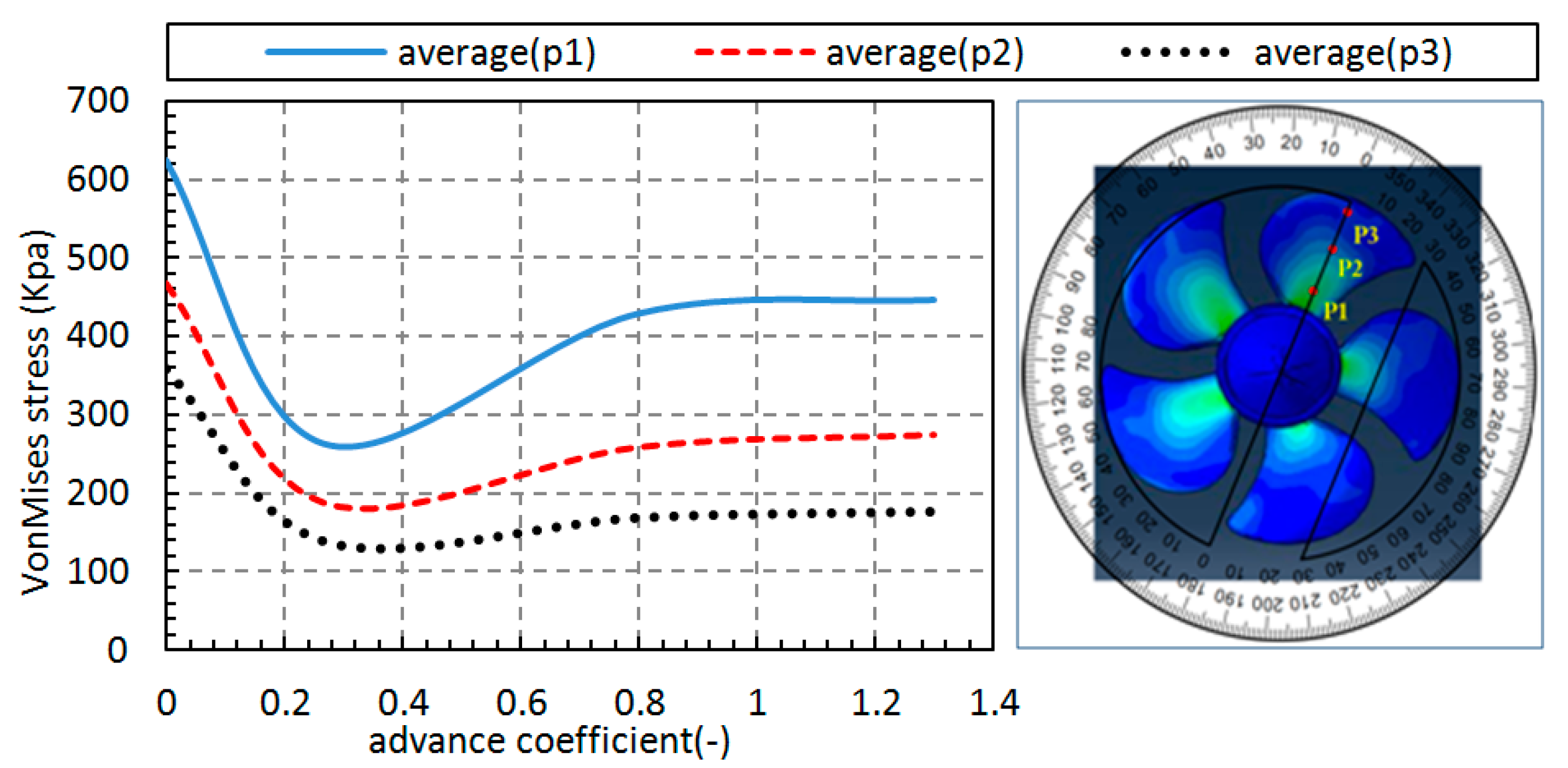
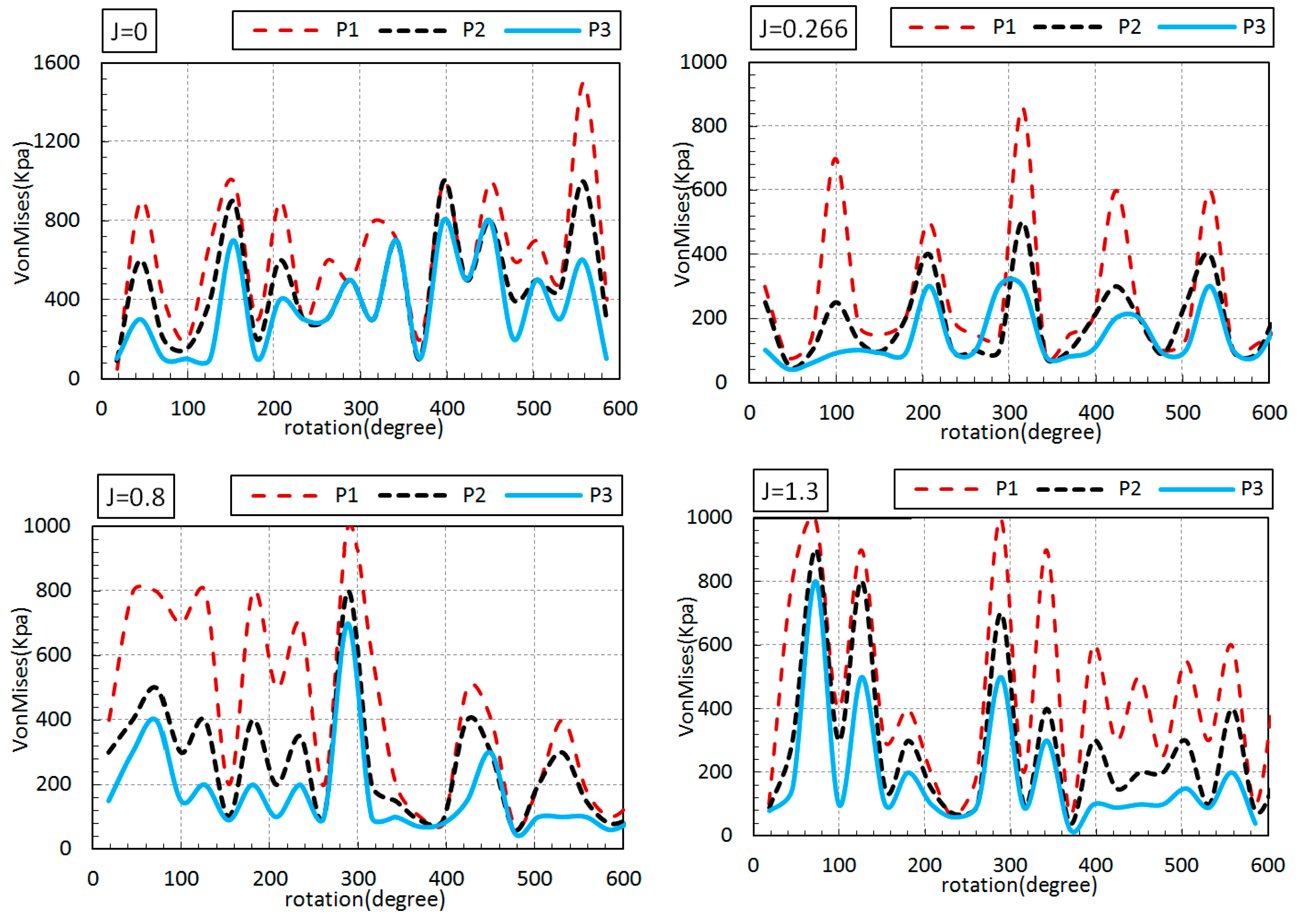
For the second step, the pressure distributions were obtained from OpenFOAM visualization software, ParaView, and used as the initial structural loads in Abaqus software. The point is that the propeller must have an appropriate rotational motion in each time-step; this procedure continued until it reaches any complete revolutions needed. Emphasis is put on von Mises stress, which is vital for evaluating the propeller’s structural strength. A fact that is borne out is that the maximum stress occurs at the bollard pull state, J = 0. In addition, j = 0.266 has the minimum stress value apart from the advance coefficient. Although von Mises stress’s value remained stable without a notable change after J = 0.8, the value and maximum stress position could be changeable for each advance coefficient under different work conditions. Consequently, the propeller’s structural behavior can effectively be analyzed by the one-way coupling approach, which is a simple, but efficient model by considering the OpenFOAM and Abaqus solvers as the CFD and FEM solutions, respectively. The present method aims to assess the appropriate material or design framework for a wide range of propellers and working conditions with an accurate and low-cost method.

Author Contributions

Conceptualization, methodology, M.M.; software, original draft preparation, M.M.; validation, A.M.; writing—review and editing, visualization, project administration, M.M. and A.M.; All authors have read and agreed to the published version of the manuscript.

Funding

This research received no funding.

Institutional Review Board Statement

Not applicable.

Informed Consent Statement

Not applicable.

Data Availability Statement

Not applicable.

Conflicts of Interest

Authors declare no conflict of interests.

Abbreviations

Arbitrary mesh interfaceAMI
Boundary element methodBEM
Computational fluid dynamicCFD
Fluid–structure interactionFSI
Finite element methodFEM
International Towing Tank ConferenceITTC
Large eddy simulationLES
Multi-reference frameMRF
Pressure implicit with splitting of operatorsPISO
Potsdam propeller test casePPTC
Vortex lattice methodVLM
Volume of fluidVOF
Reynolds-averaged Navier–StokesRANS
Rigid/quasi-staticRQS
Semi-implicit method for pressure-linked equationsSIMPLE
Turbulent kinetic energyTKE
Wetting time equationWQ

Nomenclature

K t Thrust coefficient
K q Torque coefficient
V a Advance velocity
η Efficiency
JAdvance coefficient
EElasticity
ρ Density
υPoissons’ ratio
ωAngular frequency
Svon Mises stress
P i Pressure gauge (i = 1–2–3)
εStrain
FForce
T,tTime
eError percentage
revPropeller revolution

References

  1. Young, Y.L. Hydroelastic behavior of flexible composite propellers in wake inflow. In Proceedings of the 16th International Conference on Composite Materials, Kyoto, Japan, 8–13 July 2007. [Google Scholar]
  2. Olsen, A.S. Optimisation of propellers using the vortex-lattice method. In Mechanical Engineering, Maritime Engineering; Technical Univercity Of Denmark: Lyngby, Denmark, 2002. [Google Scholar]
  3. Cokljat, D.; Caridi, D. Embedded LES methodology for general-purpose CFD solvers. In Sixth International Symposium on Turbulence and Shear Flow Phenomena; Begel House Inc.: Danbury, CT, USA, 2009. [Google Scholar]
  4. Yao, J. Investigation on hydrodynamic performance of a marine propeller in oblique flow by RANS computations. Int. J. Nav. Archit. Ocean Eng. 2015, 7, 56–69. [Google Scholar] [CrossRef] [Green Version]
  5. Krasilnikov, V.; Zhang, Z.; Hong, F. Analysis of unsteady propeller blade forces by RANS. In Proceedings of the First International Symposium on Marine Propulsors smp, Trondheim, Norway, 6 June 2009. [Google Scholar]
  6. Dubbioso, G.; Muscari, R.; Di Mascio, A. Analysis of a marine propeller operating in oblique flow. Part 2: Very high incidence angles. Comput. Fluids 2014, 92, 56–81. [Google Scholar] [CrossRef]
  7. Abdel-Maksoud, M.; Hellwig, K.; Blaurock, J. Numerical and experimental investigation of the hub vortex flow of a marine propeller. In Proceedings of the 25th Symposium on Naval Hydrodynamics, St. John’s, NL, Canada, 12 June 2004. [Google Scholar]
  8. Simonsen, C.D.; Stern, F. RANS maneuvering simulation of Esso Osaka with rudder and a body-force propeller. J. Ship Res. 2005, 49, 98–120. [Google Scholar] [CrossRef]
  9. Valentine, D.T. Reynolds-Averaged Navier-Stokes Codes and Marine Propulsor Analysis; Carderock Division, Naval Surface Warfare Center: Bethesda, MD, USA, 1993. [Google Scholar]
  10. Das, H. CFD Analysis for Cavitation of a Marine Propeller. In Proceedings of the 8th Symposium on High Speed Marine Vehicles, Naples, Italy, 22–23 May 2008. [Google Scholar]
  11. Mulcahy, N.; Prusty, B.; Gardiner, C. Hydroelastic tailoring of flexible composite propellers. Ships Offshore Struct. 2010, 5, 359–370. [Google Scholar] [CrossRef]
  12. Blasques, J.P.; Berggreen, C.; Andersen, P. Hydro-elastic analysis and optimization of a composite marine propeller. Mar. Struct. 2010, 23, 22–38. [Google Scholar] [CrossRef]
  13. Young, Y.L. Fluid–structure interaction analysis of flexible composite marine propellers. J. Fluids Struct. 2008, 24, 799–818. [Google Scholar] [CrossRef]
  14. Lee, H.; Song, M.-C.; Suh, J.-C.; Chang, B.-J. Hydro-elastic analysis of marine propellers based on a BEM-FEM coupled FSI algorithm. Int. J. Nav. Archit. Ocean Eng. 2014, 6, 562–577. [Google Scholar] [CrossRef] [Green Version]
  15. He, X.; Hong, Y.; Wang, R. Hydroelastic optimisation of a composite marine propeller in a non-uniform wake. Ocean Eng. 2012, 39, 14–23. [Google Scholar] [CrossRef]
  16. Maljaars, P.; Bronswijk, L.; Windt, J.; Grasso, N.; Kaminski, M. Experimental validation of fluid–structure interaction computations of flexible composite propellers in open water conditions using BEM-FEM and RANS-FEM methods. J. Mar. Sci. Eng. 2018, 6, 51. [Google Scholar] [CrossRef] [Green Version]
  17. Hong, Y.; Hao, L.F.; Wang, P.C.; Liu, W.B.; Zhang, H.M.; Wang, R.G. Structural design and multi-objective evaluation of composite bladed propeller. Polym. Polym. Compos. 2014, 22, 275–282. [Google Scholar] [CrossRef]
  18. Han, S.; Lee, H.; Song, M.C.; Chang, B.J. Investigation of Hydro-Elastic Performance of Marine Propellers Using Fluid-Structure Interaction Analysis. In Proceedings of the ASME International Mechanical Engineering Congress and Exposition, Houston, TX, USA, 13–19 November 2015; American Society of Mechanical Engineers: New York, NY, USA, 2015. [Google Scholar]
  19. Paik, B.-G.; Kim, G.-D.; Kim, K.-Y.; Seol, H.-S.; Hyun, B.-S.; Lee, S.-G.; Jung, Y.-R. Investigation on the performance characteristics of the flexible propellers. Ocean Eng. 2013, 73, 139–148. [Google Scholar] [CrossRef]
  20. Shayanpoor, A.A.; Hajivand, A.; Moore, M. Hydroelastic analysis of composite marine propeller basis Fluid-Structure Interaction (FSI). Int. J. Marit. Technol. 2020, 13, 51–59. [Google Scholar]
  21. Vassen, J.-M.; De Vincenzo, P.; Hirsch, C.; Leonard, B. Strong coupling algorithm to solve fluid-structure-interaction problems with a staggered approach. ESASP 2011, 692, 128. [Google Scholar]
  22. Piro, D.J. A Hydroelastic Method for the Analysis of Global Ship Response Due to Slamming Events. In Naval Architecture and Marine Engineering; University of Michigan: Ann Arbor, MI, USA, 2013. [Google Scholar]
  23. Moukalled, F.; Mangani, L.; Darwish, M. The Finite Volume Method in Computational Fluid Dynamics; Springer: Berlin/Heidelberg, Germany, 2016; Volume 6. [Google Scholar]
  24. Aagaard, O. Hydroelastic Analysis of Flexible Wedges; Department of Marine Technology, Norwegian University of Science and Technology: Trondheim, Norway, 2013. [Google Scholar]
  25. Taylor, D. The Speed and Power of Ships; Ransdell Inc.: Washington, DC, USA, 1933.
  26. Cohen, J.W. On stress calculations in helicoidal shells and propeller blades. In Mechanical, Maritime and Materials Engineering; Delft University of Technology: Delft, The Netherlands, 1955. [Google Scholar]
  27. Conolly, J. Strength of propellers. Trans. RINA 1974, 103, 139–204. [Google Scholar]
  28. Greening, P.D. Dynamic Finite Element Modelling and Updating of Loaded Structures; University of Bristol: Bristol, UK, 1999. [Google Scholar]
  29. Taghipour, R. Efficient prediction of dynamic response for flexible and multi-body marine structures. In Marine Technology; Norwegian University of Science and Technology: Trondheim, Norway, 2008. [Google Scholar]
  30. Cosden, I.A.; Lukes, J.R. A hybrid atomistic–continuum model for fluid flow using LAMMPS and OpenFOAM. Comput. Phys. Commun. 2013, 184, 1958–1965. [Google Scholar] [CrossRef]
  31. Klasson, O.K.; Huuva, T. Potsdam propeller test case (PPTC). In Proceedings of the Second International Symposium on Marine Propulsors, SMP, Hamburg, Germany, 15–17 June 2011. [Google Scholar]
  32. Khan, A.M. Flexible composite propeller design using constrained optimization techniques. In Aerospace Engineering; Iowa State University: Ames, IA, USA, 1997. [Google Scholar]
  33. Barlow, J. More on optimal stress points—reduced integration, element distortions and error estimation. Int. J. Numer. Methods Eng. 1989, 28, 1487–1504. [Google Scholar] [CrossRef]
  34. Panciroli, R. Dynamic Failure of Composite and Sandwich Structures; Springer: Dordrecht, The Netherlands, 2013; Volume 192. [Google Scholar]
  35. Heller, S.; Jasper, N. Strength on the Structural Design of Planing Craft. Available online: https://repository.tudelft.nl/islandora/object/uuid%3Adc7516f5-6d26-4419-8955-37af96d86878 (accessed on 22 March 2021).
  36. Taylor, J.L. Natural vibration frequencies of flexible rotor blades. Aircr. Eng. Aerosp. Technol. 1958, 30, 331. [Google Scholar] [CrossRef]
  37. Ekinci, S. A Practical Approach for Design of Marine Propellers with Systematic Propeller Series. Brodogr. Teor. Praksa Brodogr. Pomor. Teh. 2011, 62, 123–129. [Google Scholar]
Figure 1. Numerical solution domain used for computational fluid dynamics (CFD) part of the present study.
Jmse 09 00351 g001
Figure 2. Mesh generated structure around the propeller.
Jmse 09 00351 g002
Figure 3. Hydrodynamic comparison between experimental and numerical results.
Jmse 09 00351 g003
Figure 4. Pressure (top) and velocity (bottom) contours for different advance coefficients.
Jmse 09 00351 g004
Figure 5. Gauge pressure variations of one rotation (t = 0.12 s-t = 0.18 s) for different advanced coefficients.
Jmse 09 00351 g005
Figure 6. Integral forces act on the propeller at the different advanced coefficients.
Jmse 09 00351 g006
Figure 7. Present method (by considering the wedge impact) verification versus two-way coupling [24].
Jmse 09 00351 g007
Figure 8. The comprehensive chart of the present method by considering the solvers engaged.
Jmse 09 00351 g008
Figure 9. The comparison between a maximum stress and hydrodynamic efficiency.
Jmse 09 00351 g009
Figure 10. Maximum stress and strain values, for two revolutions, at J = 0, 0.266, 0.8, 1.23.
Jmse 09 00351 g010
Figure 11. Von Mises stress evaluation on propeller surface at different time-steps.
Jmse 09 00351 g011
Figure 12. Maximum von Mises stress on a blade versus advance coefficient.
Jmse 09 00351 g012
Figure 13. Maximum von Mises stress versus rotation angle for j = 0, 0.266, 0.8, 1.23.
Jmse 09 00351 g013
Table 1. Geometrical specification of the propeller.
Propeller ModelVp1304
Diameter0.25 m
Hub coefficient0.3
Number of blades5
pitch coefficient
(r/R = 0.7)
1.635
AE/A00.779
Table 2. Structural specification of the propeller.
MaterialAl-Alloy
Elasticity120 Gpa
Poisson’s ratio0.34
Mass density7400 kg/m3
Table 3. Primary data assumed in calculations.
ParameterUnitModelReal
Density (water)kg m−3999.01025
Kinematic viscosity (water)m2 s−11.139 × 10−61.188 × 10−6
Revolution (propeller)s−1154.33
Table 4. Mesh independency study for vp1304 propeller.
QualityBase GridCell.NUM k t ( k t ) e x c e l l e n t k q ( k q ) e x c e l l e n t NUM
Coarse0.11245,2101.11.11(I)
Mid0.09315,4021.051.055(II)
Mid-fine0.08335,1831.0251.024(III)
Fine0.064425,0601.0151.013(IIII)
Excellent0.0325835,205≈1≈1(V)
Table 5. Different advance coefficient specifications.
J [-]ω [rps]Va [m/s]Number
0.266151I
0.533152II
0.8153III
1.06154IIII
1.23155V
1.6156VI
Table 6. Three gauge positions on the propeller blade.
GaugeDistance from the Center Jmse 09 00351 i001
p-10.04 m
p-20.08 m
p-30.12 m
Table 7. Wedge characteristic used for one-way coupling verification solution.
CharactersWedge LengthWedge ThicknessDeadrise Angle
value0.3 m0.002 m20°
Table 8. Material properties for the wedge used for one-way coupling verification solution.
CharactersMaterialE [Gpa] ρ [kg/m3] ν [-]
valueAluminum6827000.3
Table 9. The datasheet for the coupling procedure of v = 5 m/s test case.
Case (FEM)1234567
Time step(s)0.070.0750.080.0850.090.0950.1
Rotation Angle18°45°72°99°126°153°180°
Stress (pa)6.01 × 1065.92 × 1065.47 × 1065.59 × 1065.91 × 1069.16 × 1065.90 × 106
Strain (m)4.7 × 10−54.67 × 10−54.34 × 10−54.4 × 10−54.6 × 10−58.4 × 10−54.6 × 10⁻⁵
89101112131415
0.1050.110.1150.120.1250.130.1350.14
207°234°261°288°315°342°369°396°
8.87 × 1058.40 × 1055.20 × 1065.70 × 1065.80 × 1065.80 × 1065.70 × 1065.70 × 106
8.2 × 10−67.8 × 10−64.11 × 10−54.5 × 10−54.6 × 10−54.59 × 10−54.56 × 10−54.56 × 10−5
1617181920212223
0.1450.150.1550.160.1650.170.1750.18
423°450°477°504°531°558°585°612°
5.70 × 1065.60 × 1065.68 × 1065.63 × 1065.60 × 1065.55 × 1065.40 × 1065.30 × 106
4.51 × 10−54.44 × 10−54.45 × 10−54.44 × 10−54.41 × 10−54.36 × 10−54.28 × 10−54.17 × 10−5
Table 10. The time needed to analyze different cases.
Advance VelocityV = (1, 2, 3, 4, 5)m/s
FEM solution time + gathering datasheet2 + 1hour
CFD solution time24hour
Cumulative time (present method)27hour
Publisher’s Note: MDPI stays neutral with regard to jurisdictional claims in published maps and institutional affiliations.

