
Dynamic Amplification of Gust-Induced Aerodynamic Loads Acting on a Wind Turbine during Typhoons in Taiwan


Abstract
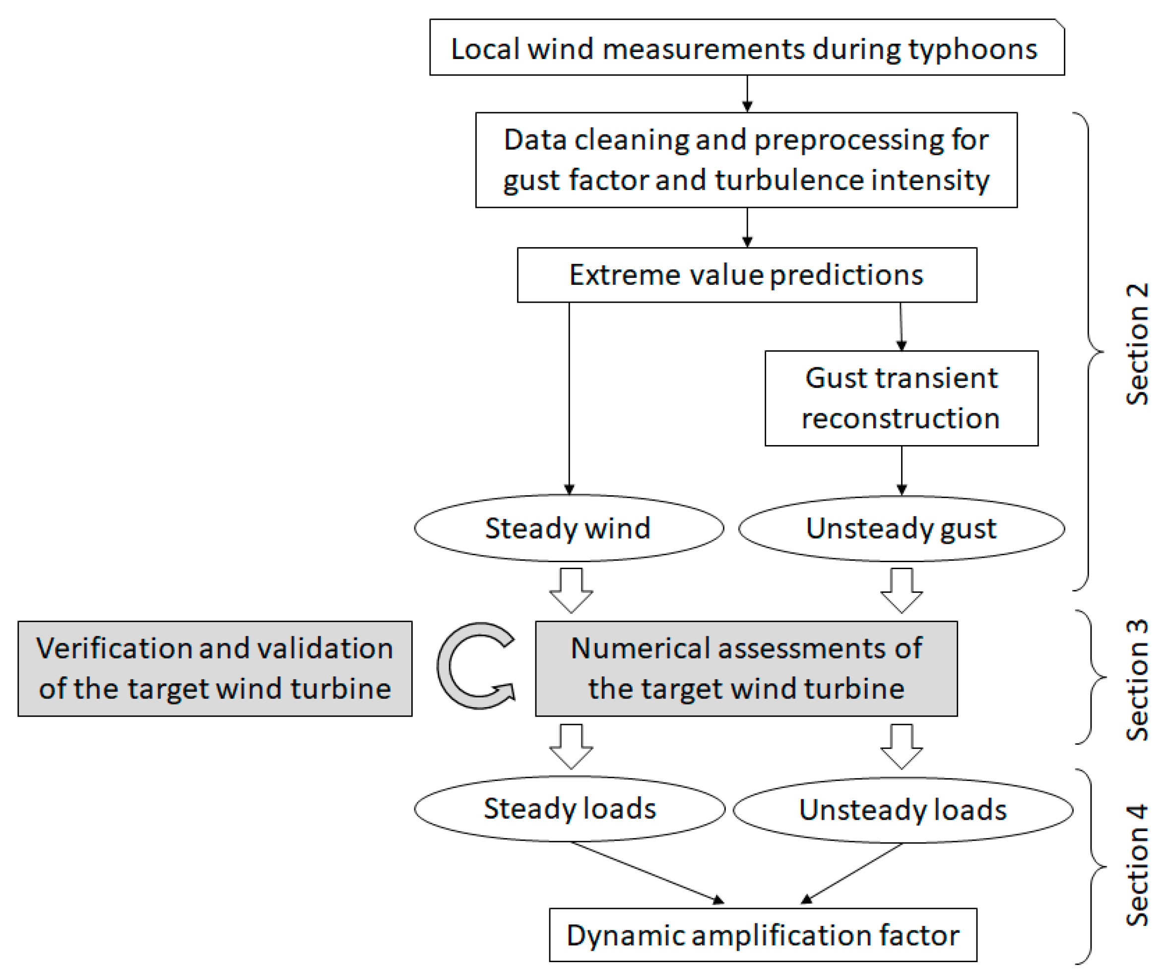
1. Introduction
2. Typhoon Wind Condition
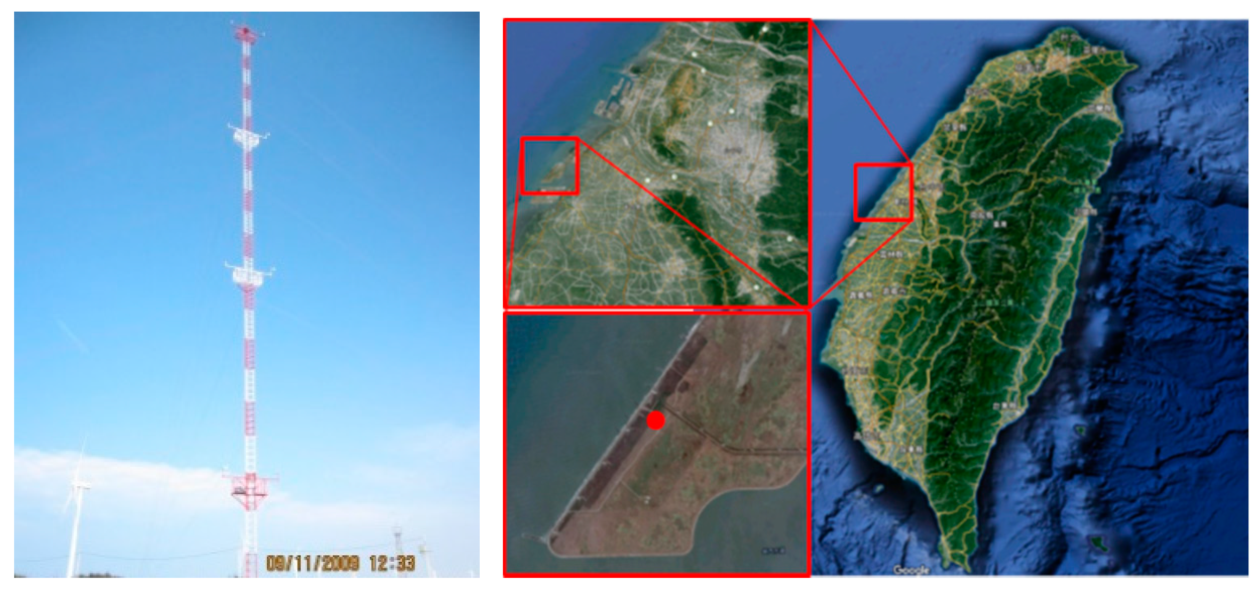
2.1. Wind Speed Measurement
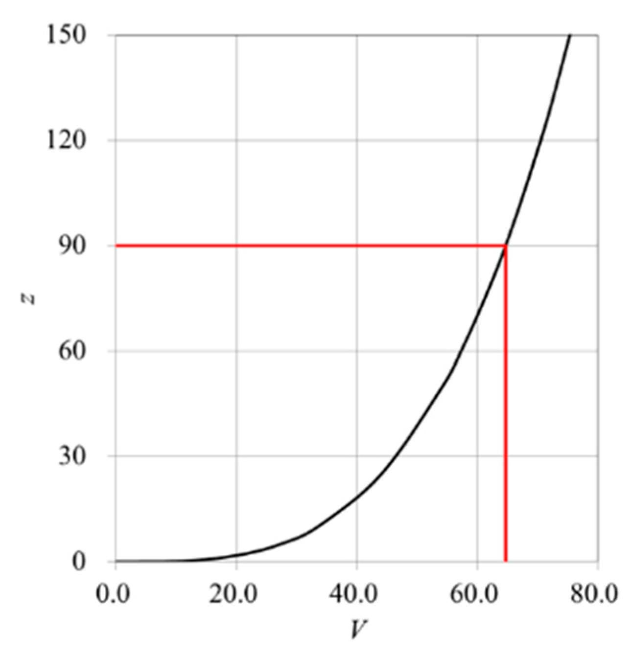
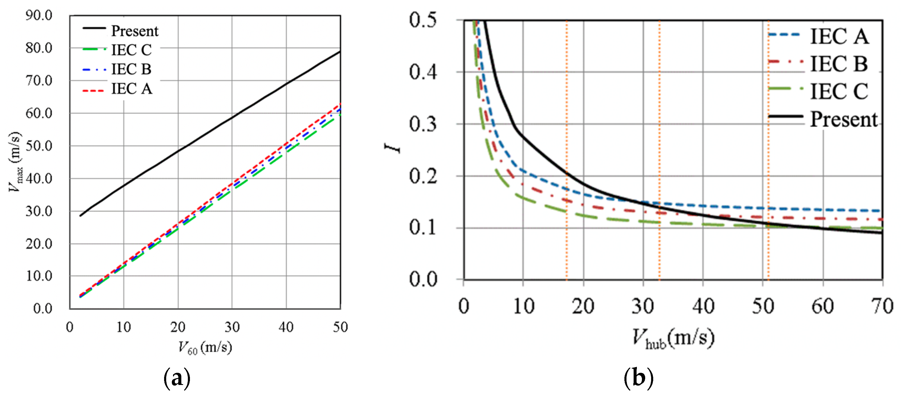
2.2. Extreme Wind Condition
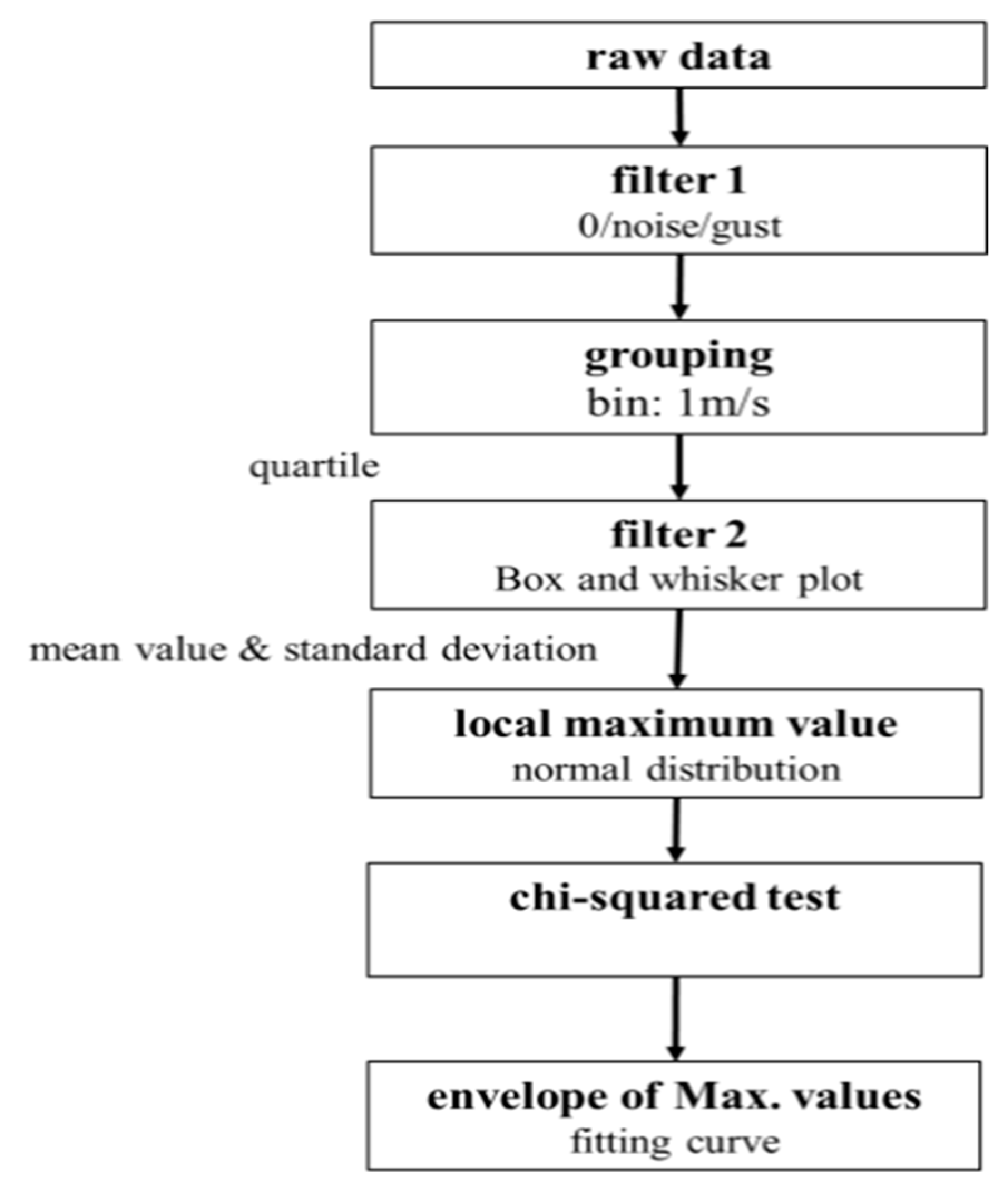
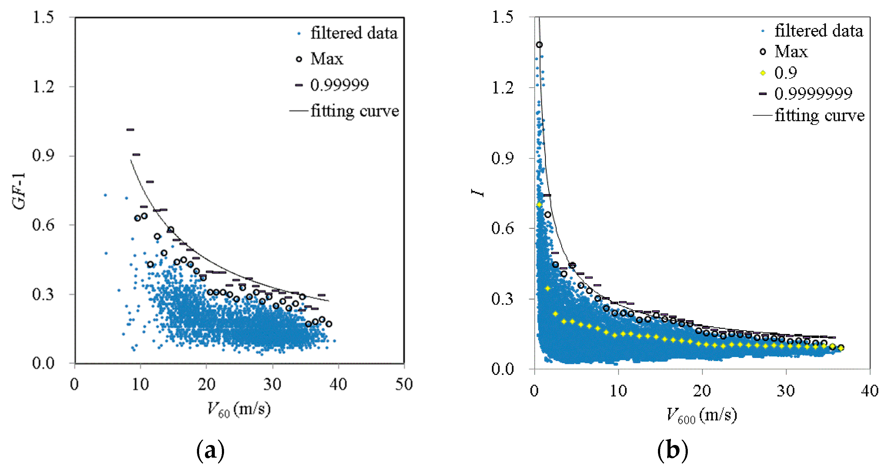
- Filter 1: The raw data were firstly filtered by removing zeros and empty fields. High-frequency noise was trimmed and low gusts that did not meet this definition were removed.
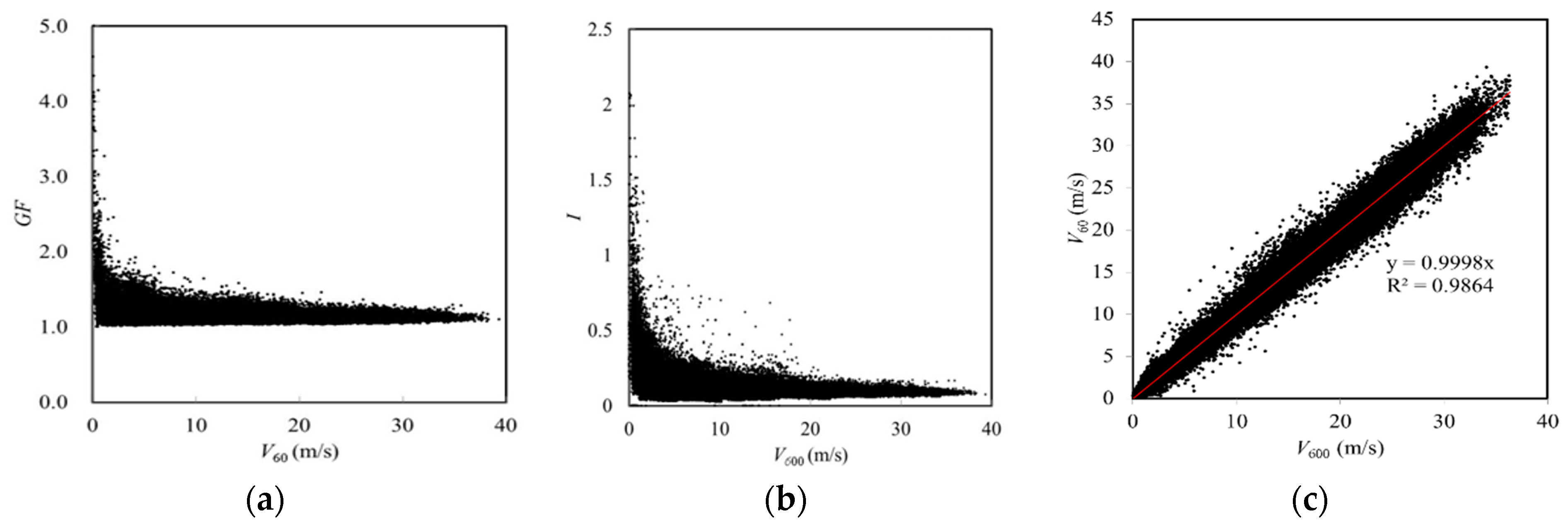
- Grouping: The recorded data were divided into 1 m/s bins, employing the 1-min average wind speeds for gust factors and 10-min average wind speeds for turbulence intensities.
- Filter 2: The data in each interval were assumed to fit a normal distribution. Unreasonable values and outliers of each interval were filtered by box-whisker plot. This filter performed the calculation of the first (Q1) and third (Q3) quartiles of the gust factor and turbulence intensity, and then the interquartile range (IQR) was computed. Data values that exceeded Q3 by three times IQR or were less than Q1 by three times IQR were identified as outliers and removed.
- Chi-squared test: The maximum cumulative probability of all the intervals filtered by chi-squared test was applied to estimate the extreme value of each interval by the assumption of normal distribution with a confidence interval of 95%.
- Fitting: The fitting curve of the estimated extreme values of each wind speed group was calculated by an exponential function with a least-squares fitting algorithm.
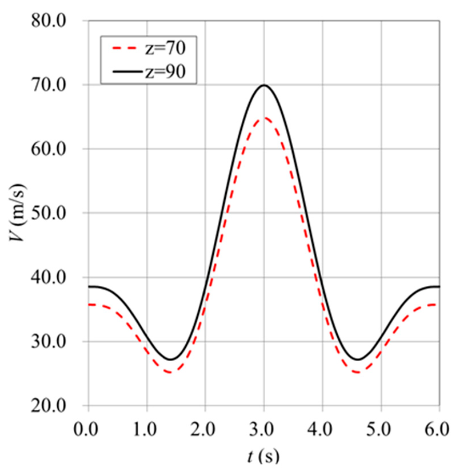
2.3. Reconstruction of Transient Gust
3. Wind Load Assessment
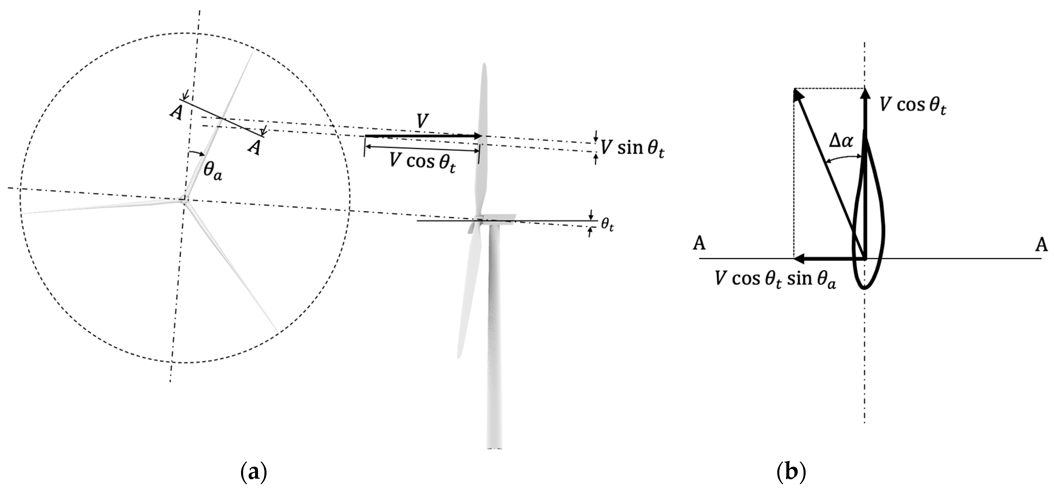
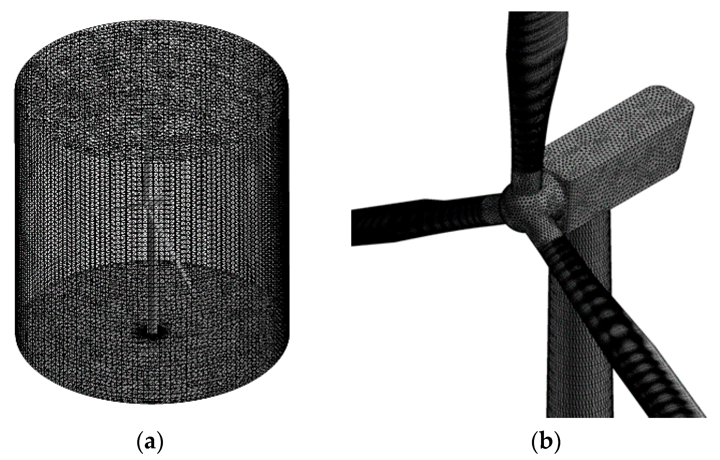
3.1. Wind Turbine Model
3.2. Numerical Method
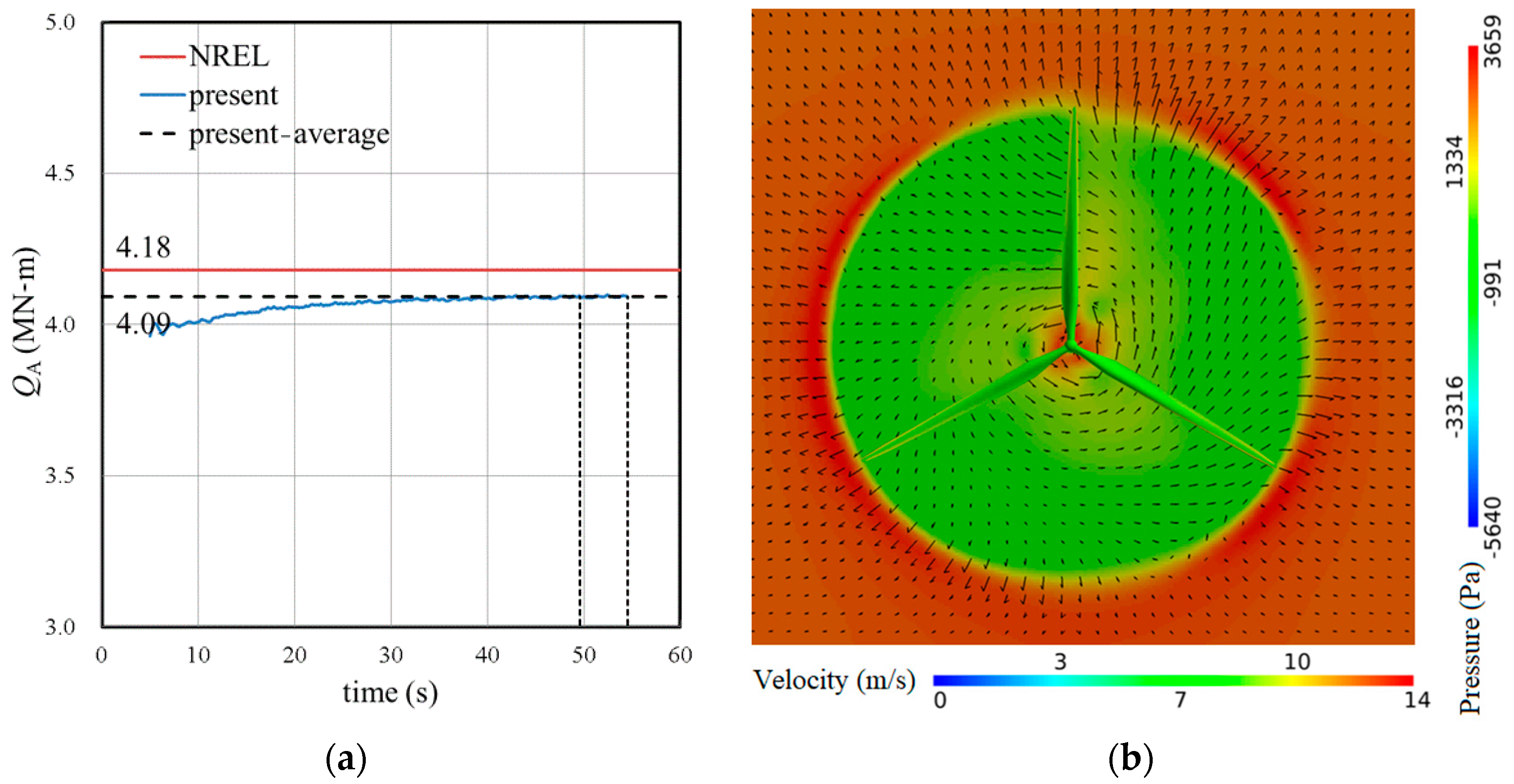
3.3. Verification and Validation
4. Results and Discussion
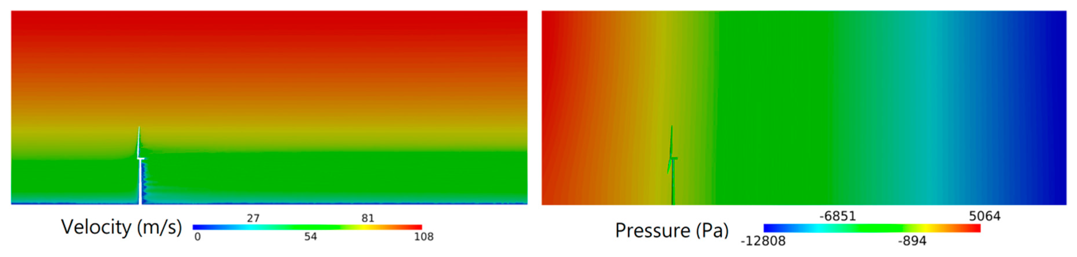
4.1. Steady Aerodynamic Loadings
4.2. Dynamic Amplification
5. Conclusions
Author Contributions
Funding
Institutional Review Board Statement
Informed Consent Statement
Data Availability Statement
Acknowledgments
Conflicts of Interest
References
- Liu, J.-H.; Chen, J.-C. Typhoon wind condition analysis—A case study to the 2 MW wind turbine during the typhoon soudelor in 2015. In Proceedings of the 15th World Wind Energy Conference and Exhibition, Tokyo, Japan, 31 October–1 November 2016. [Google Scholar]
- International Standard: Wind Turbines Part 1: Design Requirements; International Electrotechnical Commission: Geneva, Switzerland, 2005.
- Ishizaki, H. Wind profiles, turbulence intensities and gust factors for design in typhoon-prone regions. J. Wind Eng. Ind. Aerodyn. 1983, 13, 55–66. [Google Scholar] [CrossRef]
- Cao, S.; Tamura, Y.; Kikuchi, N.; Saito, M.; Nakayama, I.; Matsuzaki, Y. Wind characteristics of a strong typhoon. J. Wind Eng. Ind. Aerodyn. 2009, 97, 11–21. [Google Scholar] [CrossRef]
- Clausen, N.E.; Ott, S.; Tarp-Johnsen, N.J.; Norgard, R.; Guo, X.L. Design of wind turbine in an area with tropical cyclones. In Proceedings of the European Wind Energy Conference and Exhibition, Athens, Greece, 27 February–2 March 2006. [Google Scholar]
- Garcino, L.E.O.; Koike, T. New reference wind speed for wind turbine in typhoon-prone areas in the Philippines. J. Struct. Eng. 2010, 136, 463–467. [Google Scholar] [CrossRef]
- Ishihara, T.; Yamaguchi, A.; Takahara, K.; Mekaru, T.; Matsuura, S. An analysis of damaged wind turbines by typhoon Maemi in 2003. In Proceedings of the sixth Asia-Pacific Conference on Wind Engineering, APCWE-VI, Seoul, Korea, 12–14 September 2005. [Google Scholar]
- Uchida, T.; Maruyama, T.; Ishikawa, H.; Zako, M.; Deguchi, A. Investigation of cause of wind turbine blade damage at Shiratakiyama wind farm in Japan, a computer simulation based approach. In Reports of Research Institute for Applied Mechanics; Kyushu University: Fukuoka, Japan, 2011; pp. 13–25. [Google Scholar]
- Länger-Möller, A. Simulation of transient gusts on the NREL 5MW wind turbine using the URANS solver THETA. Wind Energy Sci. 2018, 3, 461–474. [Google Scholar] [CrossRef]
- Jonkman, J.M. Dynamics Modeling and Loads Analysis of an Offshore Floating Wind Turbine; Technical Report NREL/TP-500-41958; National Renewable Energy Laboratory: Golden, CO, USA, 2007.
- Amaechi, C.V.; Wang, F.; Hou, X.N.; Ye, J.Q. Strength of submarine hoses in Chinese-lantern configuration from hydrodynamic loads on CALM buoy. Ocean Eng. 2019, 171, 429–442. [Google Scholar] [CrossRef]
- Haddadin, S.; Aboshosha, H.; El Ansary, A.; El Damatty, A. Sensitivity of wind induced dynamic response of a transmission line to variations in wind speed. In Proceedings of the Conference of Canadian Society of Civil Engineers—Resilience Infrastructure, London, UK, 1–4 June 2016. [Google Scholar]
- Pu, Z.R. A Study of Typhoon Wind Speed Profile’s Parameters in Taiwan. Master’s Thesis, Department of Harbor and River Engineering, National Taiwan Ocean University, Zhongzheng, Taiwan, 2008. [Google Scholar]
- Harper, B.A.; Kepert, J.D.; Ginger, J.D. Guidelines for Converting between Various Wind Averaging Periods in Tropical Cyclone Condition; World Meteorological Organization: Geneva, Switzerland, 2010. [Google Scholar]
- Lin, P.H.; Tu, C.T. The characteristics of gust wind at western coast of Taiwan during typhoon weather condition—An example from typhoon. In Proceedings of the Taiwan Wind Energy Conference, Penghu, Taiwan, 17 December 2010. [Google Scholar]
- Jonkman, J.; Butterfield, S.; Musial, W.; Scott, G. Definition of a 5-MW Reference Wind Turbine for Offshore System Development; Technical Report NREL/TP-500-38060; National Renewable Energy Laboratory: Golden, CO, USA, 2009.
- Ansys® FLUENT; Release 16—User’s Guide; ANSYS, Inc.: Canonsburg, PA, USA, 2015.


| Wind Speed (m/s) | z = 70 m (Met. Height) | z = 90 m (Hub Height) |
|---|---|---|
| 35.75 | 38.55 | |
| 36.00 | 38.82 | |
| 45.36 | 48.91 | |
| 61.41 | 66.22 | |
| 64.85 | 69.93 |
| Rotor type | Upwind, 3 blades |
| Diameter () | 126 m |
| Hub height () | 90 m |
| Hub diameter () | 3 m |
| Tilt angle () | 5° |
| Pitch angle () | Operating: 0°~23.5°; Parked: 90° |
| Rated wind speed | 11.4 m/s |
| Rated rotor speed | 12.1 rpm |
| Lh | Lw | L1 | L2 | DII | HII |
|---|---|---|---|---|---|
| 3D | 3D | 2D | 6D | 1.27D | 1.31D |
| Boundary | Type | Velocity Condition |
|---|---|---|
| abcd (upstream) | Inlet | Velocity specified |
| abfe, aehd, bcgf (far field) | Inlet | Velocity specified |
| ghef (downstream) | Outlet | Zero velocity gradient |
| cdhg (ground) | No-slip wall | Zero velocity |
| Wind Turbine Surface | No-slip wall | Zero velocity |
| Load (kN/MN-m) | Part | Blade Configuration | |||
|---|---|---|---|---|---|
| 0°–120°–240° | 30°–150°–270° | 60°–180°–300° | 90°–210°–330° | ||
| Tower | 276.0 | 280.3 | 306.0 | 284.3 | |
| Rotor | 172.5 | 175.7 | 146.6 | 177.3 | |
| Total | 451.6 | 458.9 | 454.5 | 465.5 | |
| Rotor | 3.80 | 5.00 | 1.20 | 2.50 | |
| Blade 1 | −0.20 | −0.23 | −0.23 | −0.21 | |
| Blade 2 | −0.17 | −0.17 | −0.10 | −0.12 | |
| Blade 3 | −0.13 | −0.12 | −0.13 | −0.17 | |
| Tower | −3.7 | −1.6 | −10.8 | −1.2 | |
| Rotor | −1.0 | 5.2 | 1.8 | 4.0 | |
| Total | −5.0 | 3.7 | −9.1 | 3.1 | |
| Rotor | 18.1 | 18.2 | 15.8 | 17.8 | |
| Tower | 13.8 | 13.9 | 15.9 | 14.2 | |
| Total | 32.3 | 32.5 | 31.9 | 32.5 | |
| Rotor | 0.60 | 1.30 | −0.09 | 0.50 | |
| Tower | <0.001 | ||||
| Total | 0.60 | 1.30 | −0.06 | 0.60 | |
| Load (kN/MN-m) | Part | At t = 3 s | Maximum | tmax (s) |
|---|---|---|---|---|
| Tower | 400.3 | 458.5 | 2.70 | |
| Rotor | 209.8 | 223.0 | 2.86 | |
| Total | 621.3 | 693.8 | 2.74 | |
| Rotor | 5.11 | 5.31 | 2.87 | |
| Blade 1 | −0.19 | −0.19 | 3.01 | |
| Blade 2 | −0.19 | −0.19 | 3.00 | |
| Blade 3 | −0.16 | −0.16 | 2.93 | |
| Total | 0.76 | −1.78 | 2.28 | |
| Total | 39.16 | 42.04 | 2.80 | |
| Total | 0.80 | 0.84 | 3.06 |
| Load (kN/MN-m) | Gust | Steady Wind | |
| 693.8 | 451.6 | 1.54 | |
| 5.31 | 3.80 | 1.40 | |
| 0.18 | 0.167 | 1.10 | |
| 1.78 | 5.00 | 0.36 | |
| 42.04 | 32.27 | 1.30 | |
| 0.84 | 0.62 | 1.35 |
Publisher’s Note: MDPI stays neutral with regard to jurisdictional claims in published maps and institutional affiliations. |
© 2021 by the authors. Licensee MDPI, Basel, Switzerland. This article is an open access article distributed under the terms and conditions of the Creative Commons Attribution (CC BY) license (http://creativecommons.org/licenses/by/4.0/).
Share and Cite
Lin, T.-Y.; Yang, C.-Y.; Chau, S.-W.; Kouh, J.-S. Dynamic Amplification of Gust-Induced Aerodynamic Loads Acting on a Wind Turbine during Typhoons in Taiwan. J. Mar. Sci. Eng. 2021, 9, 352. https://doi.org/10.3390/jmse9040352
Lin T-Y, Yang C-Y, Chau S-W, Kouh J-S. Dynamic Amplification of Gust-Induced Aerodynamic Loads Acting on a Wind Turbine during Typhoons in Taiwan. Journal of Marine Science and Engineering. 2021; 9(4):352. https://doi.org/10.3390/jmse9040352
Chicago/Turabian StyleLin, Tsung-Yueh, Chun-Yu Yang, Shiu-Wu Chau, and Jen-Shiang Kouh. 2021. "Dynamic Amplification of Gust-Induced Aerodynamic Loads Acting on a Wind Turbine during Typhoons in Taiwan" Journal of Marine Science and Engineering 9, no. 4: 352. https://doi.org/10.3390/jmse9040352
APA StyleLin, T.-Y., Yang, C.-Y., Chau, S.-W., & Kouh, J.-S. (2021). Dynamic Amplification of Gust-Induced Aerodynamic Loads Acting on a Wind Turbine during Typhoons in Taiwan. Journal of Marine Science and Engineering, 9(4), 352. https://doi.org/10.3390/jmse9040352