Mooring-Configurations Induced Decay Motions of a Buoy

Abstract

The hydrodynamic damping of a buoy stationed with three different mooring configurations was estimated using a Navier-Stokes (NS) equations solver coupled with a dynamic mooring model. The mooring configurations comprised a catenary system, a catenary system with sub floaters, and a catenary system with sub floaters and clump weights. Systematic simulations were achieved by adopting the overset grid scheme instead of the conventional morphing grid scheme, which required regenerating the entire mesh when the buoy’s initial position changed, thereby avoiding mesh distortions and numerical instabilities. Motion decay simulations in heave, pitch, and surge were conducted with and without various mooring systems. The analyzed results comprised decaying oscillating motions, natural periods, and associated amounts of damping. The mooring systems influenced not only restoring force characteristics, but also total damping of the moored buoy, which demonstrated the importance of considering mooring-induced damping when investigating moored offshore structures.

1. Introduction

Over the past several decades, there has been a continuous stream of innovations in ocean-based structures and systems, applied not only in the oil and gas area, but also more recently in the floating offshore wind energy and wave energy sectors [1]. Furthermore, owing to the scarcity of land, very large floating structures are now being designed to cater for an increasing population in coastal areas [2]. All of these structures must maintain station; that is, their mooring systems must withstand the forces of the ocean over long asset lives in the corrosive sea–air interface, while operating under various environmental conditions.

To reliably assess floating offshore structures with mooring systems, interdisciplinary knowledge of hydrodynamics, mooring dynamics, and their interactions is required. Techniques, generally classified as potential and viscous flow solvers, when coupled with various mooring models, have been developed to analyze such systems. Although potential flow based solvers are unable to implicitly consider viscous effects, they are widely used in marine hydrodynamics due to their robustness and computational efficiency. For instance, Schellin [3] investigated the dynamics of single-point moored vessels subject to current, wind, and waves, based on the use of both frequency domain and time domain approaches. The significant nonlinearities inherent in single-point mooring systems, mainly due to hydrodynamic response and control forces as well as mooring system restoring forces, may lead to multifarious dynamic phenomena, such as self-sustained oscillations. A comparative study of the mooring loads of a moored vessel in a steady current was documented in [4]. Gutiérrez-Romero et al. [5] presented a time-domain model to solve for the dynamics of floating marine devices subject to nonlinear environmental loads with special attention to mooring dynamics.

For floating offshore wind turbines, the importance of mooring line model fidelity was studied by Hall et al. [6], whereby a low-fidelity quasi-static approach and a high-fidelity dynamic mooring line model were coupled with the potential flow based solver FAST (Fatigue, Aerodynamics, Structures, and Turbulence program). They discussed the limitations of the quasi-static mooring model under steady and stochastic operating conditions. For the offshore oil and gas industry, there is a tradition of designing mooring systems using the quasi-static approach, justified by the low responsiveness and large mass of the moored structure and its corresponding low velocities. For the wave energy sector, dynamic mooring models are preferred due to the more complex dynamics involved. Apart from station keeping, which is the primary role of the mooring system, the influence of the mooring system on the efficiency of power take-off should also be considered. Thomsen et al. [7] assessed the available numerical tools for a dynamic mooring analysis. Significant cost reductions are required for floating structures to become competitive, and one key area that has the potential for cost reduction is the mooring system [8]. For instance, for the deployment of arrays of floating wave energy converters (WECs), short mooring lines providing a small footprint allow one to install multiple devices [9]. Harris et al. [10] and Davidson et al. [11] presented overviews of different generic types of WECs and their mooring requirements. Cerveira et al. [12] studied the power generation performance of a buoy type WEC under three mooring configurations and discussed their influence on the annually captured wave energy. However, potential flow methods cannot accurately predict oscillatory motions of floating structures at their natural frequencies, because viscous effects must be approximated from simplified methods [13]. Li and Yu [14] reviewed various numerical methods used for modeling WECs, such as analytical methods, potential-flow based methods, and Navier–Stokes equation solvers. They found that potential-flow based methods are generally used for the analysis under operational conditions, albeit with a carefully selected approach to account for viscous damping.

On the other hand, an unsteady computational fluid dynamics (CFD) approach can capture the nonlinear interactions between waves and floaters, thereby revealing details of various flow effects related to floating objects. Burmester et al. [13] simulated surge decay motions to account for viscous effects of scaling, wave radiation, coupled motions, and nonlinear moorings on the hydrodynamic damping of the DeepCwind semisubmersible platform via CFD. Palm et al. [15] performed a coupled CFD mooring analysis of a moored WEC, thereby presenting a solid framework for simulating the highly nonlinear behavior of wave energy convertors. Van Rij et al. [16] assessed design loads for a WEC using both potential and CFD approaches. In comparison with experimental and CFD simulation results, the potential-flow based methods can roughly approximate the design loads. Calculations and experiments showed that mooring-induced damping may account for reduced surge and sway amplitudes in the order of 20% or more, indicating that mooring-induced damping should be taken into consideration [17].

To fully account for viscous effects and the dynamics of a mooring system, we implemented a dynamic mooring model into the open-source CFD library OpenFOAM [18] to predict hydrodynamic damping of a moored buoy [19]. The computed buoy motions, the natural periods, and the amount of hydrodynamic damping were compared with experimental measurements. For different mooring models, using quasi-static mooring models coupled with potential flow solvers or viscous flow solvers [20], we found that the hydrodynamic damping of the moored floating structure was generally underpredicted [21].

Previous work of ours [22] considered a dynamic mooring model coupled with CFD to assess the influence of three different mooring configurations on the heave motion of a buoy type WEC. The mooring configurations comprised a catenary system, a catenary system with sub floaters, and a catenary system with sub floaters and clump weights. The favorable agreement between numerical simulations and experimental measurements validated the coupled numerical approach for simulating different mooring configurations. As an extension, here, we systematically studied the effects of mooring-induced damping of different mooring configurations on decay motions for a buoy type WEC. The exact same mesh was used for all simulations with different degrees-of-freedom by adopting an overset grid scheme over the conventional morphing grid domain. For the morphing grid scheme, to numerically simulate decay motions in different degrees-of-freedom (i.e., surge, heave, and pitch) caused by the change of the floater’s initial position, the entire mesh domain had to be regenerated for each case. When simulating large motions (for instance, under rough sea conditions), the associated mesh distortions and the subsequent numerical instability had to be dealt with.

Our main objective was to systematically determine the influence of different mooring configurations on buoy motions, natural periods, and the amounts of hydrodynamic damping for various degrees-of-freedom. Our results indicated that, although the mooring systems’ restoring forces were similar, their influences on buoy motions and hydrodynamic damping deviated significantly. To optimize power take-off efficiency of WECs, one key area is to find an optimal mooring configuration tailored to the particular motion characteristics of each concept.

2. Numerical Method

2.1. The Viscous Flow Solver

The open source CFD library OpenFOAM includes a method to solve free surface flows by coupling the Navier–Stokes (NS) equations with a volume of fluid (VOF) method [23]. The solution domain is subdivided into a finite number of control volumes, which may be of arbitrary shape. The integrals are numerically approximated using the midpoint rule, the mass conservation is ensured using a pressure correction equation based on a hybrid PIMPLE approach [24], which combines the Semi-Implicit Pressure Linked Equations (SIMPLE) algorithm with the Pressure Implicit with Splitting of Operators (PISO) algorithm. Boundary volumes define the free surface, and the entire fluid domain is marked by the transport function of the volume fraction. The governing equations for an incompressible Newtonian fluid are based on the continuity and the momentum conservation equations. In integral vector notation, they are written as follows:

$$\frac{\partial }{\partial t}{{\displaystyle \int }}_V^{}\rho dV+{{\displaystyle \int }}_S^{}\rho u·ndS=0$$

(1)

$$\frac{\partial }{\partial t}{{\displaystyle \int }}_V^{}\rho udV+{{\displaystyle \int }}_S^{}\rho \left(uu\right)·ndS={{\displaystyle \int }}_S^{}T·ndS+{{\displaystyle \int }}_V^{}\rho b·ndV$$

(2)

where u is the fluid velocity field vector, n is the normal vector of S representing the surface area of the control volume V, T is the stress tension, and b is a vector describing a force per unit mass. The instantaneous local density, ρ, and dynamic viscosity, µ, are expressed in terms of water volume faction α as follows:

$$\rho =\alpha {\rho }_w+{\rho }_a\left(1-\alpha \right)$$

(3)

$$\mu =\alpha {\mu }_w+{\mu }_a\left(1-\alpha \right)$$

(4)

where subscripts w and a represent water and air, respectively. Use of the MULES (Multidimensional Universal Limiter with Explicit Solution) algorithm and an additional compressive convective term reduces numerical smearing and retains a sharp interface between water and air. At each time step, the existing velocity field converts phase fractions, and the distribution and development of the free surface is estimated using the following equation:

$$\frac{\partial }{\partial t}{{\displaystyle \int }}_V^{}\alpha dV+{{\displaystyle \int }}_S^{}\alpha u·ndS+{{\displaystyle \int }}_S^{}\alpha \left(1-\alpha \right)u_r·ndS=0$$

(5)

where $u_r$ is a velocity field normal to the interface, which stands for the artificial compression on the free surface, and where its magnitude is proportional to the instantaneous velocity. Despite the existence of this artificial compression term, the free surface may be smeared over a number of cells.

The motions of a floating body are then solved using a six degrees-of-freedom rigid body motion library. Two reference frames describe body motions, namely, the global coordinate system and the body-fixed coordinate system. Solving the nonlinear motions of a floating body entails translating and rotating it about the body-fixed coordinate system [25]. The considered external loads are the hydrodynamic force, ${\overrightarrow{\mathit{f}}}_{\mathit{H}}$, the restoring force, ${\overrightarrow{\mathit{f}}}_{\mathit{C}}$, and the linear viscous mechanical damping force, ${\overrightarrow{\mathit{f}}}_{\mathit{D}}$. With a state vector, $\overrightarrow{\mathit{r}}$, extending from the origin of global coordinate system to the body’s center of gravity, the dynamic equations are given as follows [13]:

$$M\ddot{\overrightarrow{\mathit{r}}}+D\dot{\overrightarrow{\mathit{r}}}+C\overrightarrow{\mathit{r}}={\overrightarrow{\mathit{f}}}_{\mathit{H}}$$

(6)

where M is the mass matrix, D the damping matrix, and C the stiffness matrix. As we dealt with a rigid body, the mechanical damping component was zero. The stiffness component was replaced by the forces obtained from the coupled mooring model. These equations describe a second-order nonlinear initial value problem because the hydrodynamic forces and mooring restoring forces are nonlinearly related to the motion vector $\overrightarrow{\mathit{r}}$, which are obtained by solving the Navier–Stokes equations and the nonlinear dynamic mooring model, respectively.

Although accurate results were obtained using a morphing grid scheme in our previous works [19,20], for motions in rough sea conditions large mesh deformations were reported in our subsequent study [21], which yielded skewed shapes and unacceptable aspect ratios for grid cells and, consequently, induced numerical instabilities. To dispose of these limitations and still use the same mesh for our subsequent systematic simulations, we adopted the overset mesh scheme. This grid technique defined a background grid and a body-fitted grid, allowing these grids to move independently, and it connected them at appropriate cells or points using an interpolation mechanism. Cells located outside the domain or cells that were not of interest, such as cells inside the buoy, were marked as holes and excluded from the computation. Cells surrounding the holes, called fringe cells, were treated as boundaries in each overset grid. Every fringe cell had a stencil consisting of several donor cells that provided information for the fringe cell obtained from the donor grid. The value of a variable ϕ of the fringe cell was obtained by interpolation from the donor cells:

$$\varphi ={\displaystyle \sum }_{i=1}^n{\omega }_i·{\varphi }_i$$

(7)

where ${\omega }_i$ is the weight coefficient and ${\varphi }_i$ is the donor cell value for each donor. Compared to the morphing grid approach, which required regenerating the entire mesh when the buoy’s initial position changed, the overset grid approach overcame this problem. For instance, for the three motions—heave, pitch, and surge—considered here, the buoy’s initial positions differed and, consequently, three different meshes were required, as shown in Figure 1. However, as shown Figure 2, only one mesh was needed using the overset grid approach although all meshes used exactly same background grid as the body-fitted grid. These grids were transformed to fit each motion component by simply rotating the body-fitted grid, which made it easier to simulate the other degrees-of-freedoms motions, especially the motions in waves.

2.2. The Dynamic Mooring Model

The lumped mass dynamic mooring model MoorDyn [26] was adopted, which was validated against experimental measurements by coupling it with a potential flow solver [27] and a viscous flow solver [20]. As shown in Figure 3, it combined the effects of mass, external forces, and inertial reactions at a finite number of nodes along a mooring cable. A mooring cable was modeled as a set of concentrated masses connected by massless springs. Different mooring configurations were generated by adding weights/floaters in the mooring lines. The equation of motion for each node is written as follows:

$$\left(m_i+a_{pi}+a_{qi}\right){\ddot{r}}_i=T_i+C_i+W_i+B_i+D_{pi}+D_{qi}$$

(8)

where $m_i$ is the mass matrix of node i, $r_i$ is the position vector, and $a_{pi}$ and $a_{qi}$ are the corresponding transverse added mass and tangential added mass, respectively. Symbol $T_i$ represents the tension in each line segment, $C_i$ is a numerical internal damping force to improve stability,$W_i$, is the net buoyancy force, $B_i$, is the interaction with the sea bed, and $D_{pi}$ and $D_{qi}$ are the transverse and tangential drag forces, respectively. This process is described in detail in [27], and additional information on the coupling between the mooring model and the viscous flow solver is documented in [20].

3. Test Case Descriptions

3.1. The Numerical Setups

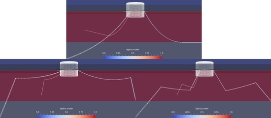
The test cases adopted from [28] were analyzed for the buoy positioned with three mooring configurations typically appropriate for WECs. Figure 4 shows an overview of the setup and the adopted mooring configurations, comprising the standard catenary system (CAT), the compact (small sea bed footprint) configuration consisting of synthetic cables and floaters (CON1), and the compact configuration made up of synthetic cables, floaters, and clump weights (CON2). The setup consisted of a cylindrical buoy moored with three mooring legs spaced 120 deg apart.

Table 1. Particulars of the moored buoy.

Mass.	Diameter	Height	Inertia 1	Center of Gravity	Draft
35.50 kg	0.515 m	0.40 m	0.95 $\mathrm{kg}·{\mathrm{m}}^2$	−0.093 m	0.174 m

¹ About horizontal axis through center of gravity.

lists the properties of the buoy without the mooring system. For the studless chain used for experimental testing, the cable diameter used in the simulations considered a volume-equivalent diameter for the mooring chain; that is, the diameter of a cylindrical cable had the same displacement per unit length as the chain [27].

Table 2. Static properties of mooring cables.

Mooring Config.	d (m)	m (kg/m)	mf (kg)	Vf (m3)	mc (kg)	Vc (m3)
CAT	0.0115	0.193	-	-	-	-
CON1	0.0060	0.035	0.250	0.0011	-	-
CON2	0.0060	0.035	0.250	0.0011	1.050	0.00005

lists the static properties for mooring simulations, namely, equivalent diameter d, mass density in air m, mass of the sub floater m_f, volume of the sub floater V_f, mass of the clump weight m_c, and volume of the clump weight V_c. The mooring model was formulated for cylindrical elements. Therefore, drag and added mass coefficients used for hydrodynamic force calculations needed to be adjusted accordingly.

Table 3. Hydrodynamic properties of mooring systems.

Symbols	Descriptions	Values
Can (-)	Transverse added mass coefficient	0.865
Cat (-)	Tangential added mass coefficient	0.269
Cdn (-)	Transverse drag coefficient	1.08
Cdt (-)	Tangential drag mass coefficient	0.213
Kbot (Pa/m)	Sea bottom stiffness	300 Pa/m
Cbot (Pa s/m)	Sea bottom damping	1.0 Pa s/m

lists the associated hydrodynamic properties adopted for the mooring simulations;

Table 4. Mean cable tensions in the buoy’s rest position.

Configurations	FREE	CAT	CON1	CON2
Tension (N)	-	3.18	3.11	10.93

, the resulting mooring tensions at the buoy’s rest position.

A rectangular box shown in Figure 5 defined the computational domain, which consisted of three domain layers. One uniform high-resolution middle layer, extending below and above the calm water level, encapsulated minimum and maximum surface elevations. The two other layers extended from the clam water level to the bottom and the top of the domain. The gridding became coarser towards to the outlet boundary to dampen wave reflections and to significantly reduce the computational effort for further simulations in waves. The distance from the inlet boundary to the buoy was about 5 D_B, where D_B is the diameter of the buoy. The distance from the outlet boundary to the buoy was about 10 D_B. The width of the wave tank was 6 D_B, and the water depth was the same as in the experiments. Figure 6 shows a sample grid topology. Grids were refined towards the free surface and towards the buoy, but their refinement was constant in the vertical direction.

3.2. Discretization Uncertainties

Numerical results from field methods are sensitive to spatial and temporal discretization uncertainties. Specifically, results from CFD simulations are subject to discretization uncertainties, iterative uncertainties, statistical uncertainties, and residual uncertainties. As our residual uncertainties turned out to be two orders of magnitude less than our discretization uncertainties, we neglected to determine the iterative uncertainties [29]. We also did not consider statistical uncertainties, because our numerically simulated decay motions resulted in time-accurate oscillating amplitudes. Therefore, we only addressed discretization uncertainties.

We started with the decaying heave motion. For our temporal uncertainty study, we adopted a refinement factor of $c_t=2.0$ and defined three time-step sizes based on a system’s natural heave period T, with $∆t_1=T/140$, $∆t_2=T/280$, $∆t_3=T/560$. A uniform refinement factor of $c_g=1.2$ was specified for all spatial directions. Consequently, the ratios specifying the number of cells for the coarse grid $G_1$, the medium grid $G_2$, and the fine grid $G_3$ were adequately matched with the factor $c_g{}^3$.

Table 5. Cell grid ratios and the associated number of cells for each grid.

Grid	Length $\mathbf{∆}\mathit{x}$(m)	Width $\mathbf{∆}\mathit{y}$(m)	Height $\mathbf{∆}\mathit{z}$	No. of Cells (-)
$G_1$	$∆x_2\times c_g$	$∆y_2\times c_g$	$∆z_2\times c_g$	$1.35\times {10}^6$
$G_2$	$∆x_2$	$∆y_2$	$∆z_2$	$2.29\times {10}^6$
$G_3$	$∆x_2/c_g$	$∆y_2/c_g$	$∆z_2/c_g$	$4.17\times {10}^6$

lists these cell grid ratios and the associated number of cells for each grid.

According to the International Towing Tank Conference (ITTC) [30], the discretization uncertainty $U_D$ was expressed as follows:

$$U_D{}^2=U_T{}^2+U_G{}^2$$

(9)

where $U_T$ and $U_G$ are uncertainties of time step size and grid size, respectively. The convergence ratio R, defined as the ratio of the difference between solutions obtained on the fine and medium grids, ${\epsilon }_{32}$, and the difference of these solutions obtained with the medium and coarse time step sizes, ${\epsilon }_{21}$, was calculated as follows:

$$R={\epsilon }_{32}/{\epsilon }_{21}$$

(10)

The asymptotic analysis from subfigures (b) and (c) of Figure 7 shows that monotonic convergence ($0<R<1$) was achieved for both target solutions, i.e., for amplitudes as well as for periods. For results with monotonic convergences, the Richardson extrapolation was applied, and the estimated numerical error ${\delta }_{RE}$ and the order of accuracy p were calculated. With three solutions, only the leading term was estimated, which provided the following one-term estimates:

$$p=\ln \left(\frac{1}{R}\right)/\ln \left(c_t\right)$$

(11)

$${\delta }_{RE}={\epsilon }_{32}/\left(1-c_t{}^p\right)$$

(12)

To better estimate the uncertainties of solutions far from the asymptotic range, the correction factor, $C_F$, was adopted [31] as a measure defining the distance of solutions from the asymptotic range:

$$C_F=\left(1-c_t{}^p\right)/\left(1-c_t{}^{p_0}\right)$$

(13)

where $p_0$ is an estimate for the limiting order of accuracy as the time-step size approaches zero, and $p_0=2$ was adopted here for a second-order accurate method. The numerical error ${\delta }_D$, the numerical benchmark result $S_C$, and the uncertainty $U_D$ were obtained from as follows:

$${\delta }_D=C_F{\delta }_{RE}$$

(14)

$$S_C=S-{\delta }_D$$

(15)

$$U_D=\left\{\begin{array}{cc}\hfill \left(2.4{\left(1-C_F\right)}^2+0.1\right)\left|{\delta }_{RE}\right|,& \left|1-C_F\right|<0.25\hfill \\ \hfill \left|1-C_F\right|\left|{\delta }_{RE}\right|,& \left|1-C_F\right|>0.25\hfill \end{array}\right.$$

(16)

where S is the final solution for the verification study. For $C_F$ significantly less than or greater than unity, the solutions are far away from the asymptotic range, and the numerical uncertainty was then calculated as follows:

$$U_D=\left\{\begin{array}{cc}\hfill \left(9.6{\left(1-C_F\right)}^2+1.1\right)\left|{\delta }_{RE}\right|,& \left|1-C_F\right|<0.125\hfill \\ \hfill \left(2\left|1-C_F\right|+1\right)\left|{\delta }_{RE}\right|,& \left|1-C_F\right|>0.125\hfill \end{array}\right.$$

(17)

Figure 7 plots results of the associated time-step size study for free heave obtained on the medium grid using three different time steps. As hydrodynamic damping and natural periods of the buoy were of interest here, the associated oscillation amplitude over one period, plotted in Figure 7b, and the corresponding time instances (periods), plotted in Figure 7c, were considered to be solutions of our verification study. The resulting phases and amplitudes, using a coarse-time step, only slightly differ from each other. Furthermore, phases and amplitudes using medium and fine time-step sizes are nearly the same.

Table 6. Time-step uncertainties of free heave motion.

Solutions	R	p	${\mathit{C}}_{\mathit{F}}$	${\mathit{S}}_{\mathit{C}}$	${\mathit{U}}_{\mathit{D}}$$(\%{\mathit{S}}_{\mathit{C}})$	${\mathrm{Diff}}_{\mathrm{C}}$	${\mathrm{Diff}}_{\mathit{M}}$	${\mathrm{Diff}}_{\mathrm{F}}$
Amplitude	0.5448	0.8762	0.2785	−0.0414	0.2203	9.76%	4.11%	1.03%
Period	0.5000	1.0000	0.3333	1.1307	0.5333	1.18%	0.47%	0.12%

lists the obtained time-step uncertainties. For both selected solutions, the convergence factors, R, are between 0 and 1, indicating that a monotonic convergence was achieved for both solutions. Time-step uncertainties for the amplitude and the period were $0.2203\%S_C$ and$0.533\%S_C$, respectively. As seen, the difference $\mathrm{Diff}{.}_{\mathrm{M}}$ between solutions obtained with the medium time-step size and the numerical benchmark solution $S_C$ was 4.11% for the amplitude and 0.47% for the period. To obtain sufficiently accurate, yet cost effective solutions, we subsequently used the medium time-step size.

To determine the grid uncertainties, we performed simulations on three different grids with the selected medium time-step, and the associated results are plotted in Figure 8. As seen, the results on different grids are almost identical, although there are small deviations between phases. Following the same procedure, the uncertainties were calculated for the oscillation amplitude and the period, and their results are listed in

Table 7. Grid uncertainties of free heave motion.

Solutions	R	p	${\mathit{C}}_{\mathit{F}}$	${\mathit{S}}_{\mathit{C}}$	${\mathit{U}}_{\mathit{D}}$$(\%{\mathit{S}}_{\mathit{C}})$	${\mathrm{Diff}}_{\mathrm{C}}$	${\mathrm{Diff}}_{\mathit{M}}$	${\mathrm{Diff}}_{\mathrm{F}}$
Amplitude	0.0300	19.2290	73.4315	−0.0432	0.0095	−1.80%	−0.16%	−0.11%
Period	0.5000	3.8018	2.2727	1.1491	1.0182	−1.84%	−1.14%	−0.79%

. Both selected solutions achieved a monotonic convergence. The uncertainties of grid size for the amplitude and the period were $0.0095\% S_C$ and $1.0182\% S_C$, respectively. Combining the time-step and grid uncertainties, the associated total discretization uncertainties were $0.2205\% S_C$ for the oscillation amplitude and $1.1494\% S_C$ for the period, which verified that our chosen time-step and grid sizes were small enough to obtain reliable predictions. The similar $\mathrm{Diff}{.}_{\mathrm{M}}$ and $\mathrm{Diff}{.}_{\mathrm{F}}$ indicate that decreasing the grid size from medium to fine did not significantly improve the results. Therefore, we chose the medium time-step and grid sizes for subsequent decay simulations.

To ensure that the chosen time-step and grid size were also applicable for decay motions in pitch and surge, we again conducted grid sensitivity studies, and the associated time series are plotted in Figure 9. As seen, the medium time-step and the medium grid size obtained accurate enough results for decay motions in pitch and surge.

3.3. Hydrodynamic Damping

The evaluation of the results comprised not only the buoy motions and mooring forces, but also the systems’ associated natural periods and amounts of hydrodynamic damping. Various techniques exist to obtain hydrodynamic damping from decay tests. Previously [19], we used an improved P-Q method to estimate linear and quadratic damping of a moored buoy and found the results to be reliable although they were sensitive to data input. Alternately, the equivalent linear damping approach [32] was adopted in this study, as it is relatively simple and robust. The nonlinear motion equation of a floating unit can be written as follows:

$$\mathrm{M}\ddot{\mathrm{x}}+B\left(\dot{\mathrm{x}}\right)+\mathrm{Cx}={\mathrm{F}}_{\mathrm{ext}}\left(\mathrm{t}\right)$$

(18)

where M is the mass, C is the stiffness, and x, $\dot{\mathrm{x},}$ and $\ddot{\mathrm{x}}$ are the motion, velocity and acceleration vectors, respectively. Vector ${\mathrm{F}}_{\mathrm{ext}}$ comprises the external forces, and the higher order nonlinear damping function, B, can be expressed as follows:

$$B={\mathrm{B}}_1\dot{\mathrm{x}}+{\mathrm{B}}_2\dot{\mathrm{x}}\left|\dot{\mathrm{x}}\right|+{\mathrm{B}}_2{\dot{\mathrm{x}}}^3+\cdots$$

(19)

For the free decay tests, considering only the linear damping and no external forces, the equation of motions in non-dimensional form can be rewritten as follows:

$$\ddot{\mathrm{x}}+2\mathsf{\zeta }{\omega }_{\mathrm{n}}\dot{\mathrm{x}}+{\omega }_{\mathrm{n}}{}^{2}x=0$$

(20)

where $\mathsf{\zeta }$ is the percentage of critical damping, and ${\omega }_{\mathrm{n}}$ is the natural frequency of the motion. Then, Equation (18) then is linear, and its solution can be rewritten as follows:

$$\mathrm{x}=x_0{e}^{-\mathsf{\zeta }{\omega }_{\mathrm{n}}t}\cos \left(\sqrt{1-{\mathsf{\zeta }}^2}{\omega }_{\mathrm{n}}t\right)$$

(21)

where $x_0$ is the initial condition of motion. An exponential fitted curve, adjusted using a least-squares approach and the parameters a and b from the exponential fit, can be found as follows:

$$\mathrm{x}=x_0{e}^{-\mathsf{\zeta }{\omega }_{\mathrm{d}}t}=a{e}^{-\mathrm{b}t}$$

(22)

where ${\omega }_{\mathrm{d}}$ is the damped natural frequency obtained from the oscillations of free decay tests.

4. Results

4.1. Decay Tests in Heave

All decay tests were simulated as a one degree-of freedom system, i.e., the influences of other motion components were not considered.

We performed four heave decay tests, namely, one test without a mooring system (FREE) and three tests with mooring configurations CAT, CON1, and CON2. Heave decay tests began by displacing the buoy a vertical distance of −0.076 m from its static equilibrium position. After it was released, it began to oscillate at its damped natural frequency about this equilibrium position. Hydrodynamic damping caused the oscillating amplitudes to decrease. Figure 10 shows plots of the numerically simulated time series of the decaying heave motion and Figure 11 shows the associated time series of tension in cable 1. Due to symmetry, only the tensions in cable 1 were plotted. As seen, due to the differing mooring restoring forces provided by the three mooing configurations, the buoy’s vertical heave motions and the tensions in cable 1 differ significantly. Heave motions and cable tensions all oscillate about their mean values. The presence of a mooring system caused heave amplitudes to decrease and that this decrease became successively more pronounced for the configurations CON1, CAT, and CON2. The buoy’s draft changed with different mooring configurations, as well as the mooring tensions. Cable tensions obtained from simulations with configurations CAT and CON1 are similar, although the amplitude peaks with the CAT system are slightly larger than those with the CON1 system. The CON2 system’s tension amplitudes are largest because this system provided the highest restoring forces.

To quantify the influence of attached mooring systems on the buoy’s hydrodynamics, the natural period, the percentage of critical damping, the computed and fitted time series of heave decay together with the envelope curves joining the computed heave amplitudes are depicted in Figure 12. Solid lines identify the computed heave motions; dotted lines, the fitted heave motions, which we obtained via the least-squares method by appropriately fitting each system’s natural period, T_p, and its percentage of critical damping, ζ. The dashed lines identify the envelope curves joining the fitted decaying heave amplitudes. Legends in the four graphs of this figure specify the natural periods and the percentages of critical damping associated with each system.

Table 8. Comparative changes of each system’s natural period, $T_p$, of the percentage of critical damping, ζ, and the mean draft caused by the presence of the mooring systems obtained from decay tests in heave.

FREE	CAT (%)	CON1 (%)	CON2 (%)
$T_p$	−0.18	−0.18	−0.44
ζ	1.83	0.34	11.99
Mean draft	−1.82	−0.57	−7.37

lists the corresponding changes of each system’s natural period, its percentages of critical damping, and the buoy’s draft brought about by the presence of the moorings.

We see that the buoy’s draft increased due to the presence of the moorings for all configurations. However, the effect of the mooring system on natural periods was minor because the mooring systems’ restoring forces were relatively small compared to the buoy’s hydrostatic restoring force, as this hydrostatic restoring force dominated the natural periods in heave. On the other hand, the systems’ damping turned out to be significant. Overall, the CON1 system had the least effect and the CON2 system had the greatest effect on heave amplitudes. Although the CAT system did influence heave motions, its effect was similar to that of the CON1 system. This was because the top part of the mooring cables of the CON1 configuration was horizontally connected to the buoy, thereby minimizing this system’s vertical force components. On the other hand, with the CON2 system, the sub floater and the clump weight attached to the mooring cables introduced additional effects.

4.2. Decay Tests in Pitch

The decay tests in pitch started with the buoy displaced at a pitch angle of 10 deg from its static equilibrium position. Figure 13 shows plots of the associated time series of computed decaying pitch motions for the free buoy and for the buoy moored with systems CAT, CON1, and CON2. Figure 14 shows plots of the corresponding time series of tension in mooring cables 1 and 2, and Figure 15 plots the process of obtaining the natural periods and damping ratio. Again, legends in the four graphs of this figure specify the natural periods and the percentages of critical damping associated with each system.

Table 9. Comparative changes of each system’s natural period, $T_p$, and of each system’s percentages of critical damping, ζ, caused by the presence of the mooring systems, obtained from decay tests in pitch.

Diff. to FREE	CAT (%)	CON1 (%)	CON2 (%)
$T_p$	−1.29	−2.23	−0.86
ζ	42.79	54.23	122.64

lists the corresponding changes of each system’s natural period and of the associated percentage of critical damping.

From Figure 13 we see that the presence of moorings caused pitch amplitudes to decrease and that this decrease became successively more pronounced for the CAT, CON1, CON2 configurations. The effects of the moorings on decaying pitch motions differed slightly from those of the decaying heave motions, in that the associated natural periods also decreased. This was because the changes of the percentage of critical pitch damping (see Table 8) were about two orders of magnitude larger compared to the percentage of critical heave damping (see Table 9).

Mooring systems provide not only a translational (horizontal) restoring force, but also a rotational restoring moment. In our model, this restoring moment was largely due to the buoy’s hydrostatic restoring moment in pitch. Although the mean tensions in cable 2 of the CAT and the CON1 systems are similar (see Figure 14), the oscillating tension amplitudes of the CON1 system greatly exceed those of the CAT system. The CON2 system caused only moderate tension amplitudes, although it has the largest tensions. All three mooring configurations induced damping that caused pitch motions to decay. In contrast to the decay motions in heave, apart from potential damping, viscous damping was largely responsible for the decay of pitch motions. Consequently, the effects of mooring-induced damping were more pronounced. Overall, the CAT system had the least effect on the pitch motions, the CON2 system had the greatest effect on damping, and the CON1 system had the greatest effect on the natural period.

4.3. Decay Tests in Surge

To compare the additional mooring-induced damping for decay motions in surge, we introduced a quasi-static mooring model as a comparison. The dynamic effects on the mooring lines were ignored in this approach, omitting the motion dependency of mass, damping, and fluid acceleration on mooring lines. Mooring line shape and tension were derived from the catenary formulation, based on the assumption that each mooring line is in static equilibrium at each time step and that inertia effects can be neglected. For further details of the adopted quasi-static (QS) model, see [21]. Figure 16 plots tensions in cables 1 and 2 for the QS and the CAT system against the buoy’s offset from its equilibrium position, whereas the QS restoring force characteristics were designed according to the CAT. As seen, their functional relationships hardly differ, which justified our decision of selecting the QS restoring force characteristics.

Figure 17 shows plots of the resulting numerically simulated time histories of surge motions obtained with restoring characteristics from the QS analysis and with restoring characteristics for the CAT, the CON1, and the CON2 mooring configurations. As seen, with restoring characteristics from the QS analysis, we obtained the largest surge amplitudes and the smallest natural period, and with the CON1 system, we found the smallest amplitudes; however, with the CAT system, we determined the largest natural period. To demonstrate the difference between mooring configurations, the simultaneously recorded mooring tensions are plotted as time histories in Figure 18, and the associated natural periods and percentages of critical damping are estimated in Figure 19.

Table 10. Comparative changes of each system’s natural period, $T_p$, and of each system’s percentage of critical damping, ζ, caused by the presence of the mooring systems obtained from decay tests in surge.

Diff. to QS	CAT (%)	CON1 (%)	CON2 (%)
$T_p$	10.45	6.47	7.15
ζ	109.90	650.00	245.83

lists the corresponding changes of each system’s natural period and of the associated percentage of critical damping.

In terms of mooring forces, although the simulation with QS analysis obtained the largest mooring forces, it also provided the smallest additional damping to the motions in surge, which demonstrated the advances of the dynamic mooring model over the quasi-static mooring model when predicting the hydrodynamic damping of a moored offshore structure. The simulation with the CAT system had the least effect and the simulation with the CON1 system the greatest effect on decaying surge motions. The simulation with the CON2 system had a medium effect on decaying surge motions because the cable tensions of this system were relatively larger, as each mooring leg incorporated not only a clump weight, but also a submerged floater. CON1 suffers the smallest mooring forces, but its force amplitudes are comparative to those from CON2. For cable tensions obtained with the CON1 system, although its amplitudes were not large, the almost horizontally acting mooring cable transmitted a relatively large horizontal force to the buoy, and this force was dominant for the decaying surge motion amplitudes and periods.

5. Conclusions

To account for mooring-induced damping, a freely floating buoy and a buoy positioned with three different mooring configurations were simulated using a Navier–Stokes equations solver coupled with a dynamic mooring model. This method allows one to consider nonlinear mooring-induced phenomena, fluid structure interactions, and the associated viscous effects.

Motion decay simulations in heave, pitch, and surge were considered. The analyzed response comprised the decaying oscillating motions, the natural periods, and the associated amount of system damping. The main objective was to systematically determine the influence of these mooring configurations on buoy motions, the systems’ natural periods, and the amount of hydrodynamic damping for heave, pitch, and surge motions. To achieve this, we performed numerical decay simulations using an overset grid scheme of exactly the same mesh for each motion component. Although the restoring force characteristics of all mooring systems considered were similar, their influence on the buoy’s motions as well as on the amounts of system damping showed large deviations.

To consider the mooring-induced damping of a moored floating structure, a dynamic mooring model must be adopted over a quasi-static mooring model. This was so because the quasi-static approach assumes that the motion of the system is uniform and linear between two static positions over a given time step and that the loads acting on the system are constant. The dynamic effects on mooring lines are ignored in this approach, omitting the motion dependency of mass, damping, and fluid acceleration on mooring lines. Larger discrepancies were expected between results obtained from the dynamic and the quasi-static mooring model when considering the oscillatory motions of a moored buoy in waves, especially for the high frequency motions. However, high velocities may happen, possibly leading to undesirable snap loads in mooring lines. If that happens, the associated mooring dynamics violate the assumption of a quasi-static mooring model.

The influence of mooring-induced damping on a moored buoy was demonstrated. This kind of damping varied significantly between configurations although the comparative mooring tensions hardly differed. The CAT system balanced the effects on the buoy’s heave, pitch, and surge motions. However, its relatively large footprint restricts its application in densely packed array formations. The CON1 system mainly restricted the buoy’s horizontal motions, but it hardly affected the buoy’s heave motion, suggesting that this kind of mooring configuration might be appropriate to position WECs that extract wave energy from vertical motions. The CON2 system restricted vertical motions more than the other systems considered.

Generally, a mooring configuration should be tailored to the particular characteristics of the floating concept. The different mooring systems considered not only influenced the system’s restoring force characteristics, but also the overall amount of damping in the system. Unlike in the offshore oil and gas sector, where large mass moored structures are characterized by low responsiveness and nearly linear load-extension restoring characteristics, moored WECs are likely to operate in a nonlinear load-extension range. For WECs, a mooring configuration is more problematic because the system’s influence on power take-off efficiency has to be considered. Such mooring configurations must be designed to optimize the power take-off efficiency of WECs, and their physical parameters have to be tailored to the particular characteristics of each concept. To optimize the power take-off efficiency of such devices, one key area, for example, might be the system’s footprint on the ocean floor, especially if a large number of converters are to be situated in a restricted area.

References

1. Jiang, C.; Chiba, S.; Waki, M.; Fujita, K.; el Moctar, O. Investigation of a Novel Wave Energy Generator Using Dielectric Elastomer. In Proceedings of the International Conference on Offshore Mechanics and Arctic Engineering, Virtual, Online, 3–7 August 2020; p. 84416. [Google Scholar]
2. Lamas-Pardo, M.; Iglesias, G.; Carral, L. A review of very large floating structures (VLFS) for coastal and offshore uses. Ocean. Eng. 2015, 109, 677–690. [Google Scholar] [CrossRef]
3. Schellin, T.E. Dynamics of single point mooring configurations. In Proceedings of the International Maritime Conference, Singapore, 24–25 September 2007. [Google Scholar]
4. Schellin, T.E. Mooring load of a ship single-point moored in a steady current. Mar. Struct. 2003, 16, 135–148. [Google Scholar] [CrossRef]
5. Gutiérrez-Romero, J.E.; García-Espinosa, J.; Serván-Camas, B.; Zamora-Parra, B. Non-linear dynamic analysis of the response of moored floating structures. Mar. Struct. 2016, 49, 116–137. [Google Scholar] [CrossRef] [Green Version]
6. Hall, M.; Buckham, B.; Crawford, C. Evaluating the importance of mooring line model fidelity in floating offshore wind turbine simulations. Wind Energy 2014, 17, 1835–1853. [Google Scholar] [CrossRef]
7. Thomsen, J.B.; Eskilsson, C.; Ferri, F. Assessment of Available Numerical Tools for Dynamic Mooring Analysis: WP1.2 & M1; DCE Technical Reports No. 220; Department of Civil Engineering, Aalborg University: Aalborg, Denmark, 2017. [Google Scholar]
8. Fitzgerald, J. Position Mooring of Wave Energy Converters. Ph.D. Thesis, Chalmers University of Technology, Goteborg, Sweden, 11 November 2009. [Google Scholar]
9. Johanning, L.; Smith, G.H.; Wolfram, J. Towards design standards for WEC moorings. In Proceedings of the 6th European Wave and Tidal Energy Conference, Glasgow, Scotland, 1 January 2005. [Google Scholar]
10. Harris, R.E.; Johanning, L.; Wolfram, J. Mooring systems for wave energy converters: A review of design issues and choices. In Proceedings of the 3rd International Conference on Marine Renewable Energy, Blyth, UK, 7–9 July 2004. [Google Scholar]
11. Davidson, J.; Ringwood, J.V. Mathematical modeling of mooring systems for wave Energy converters—A review. Energies 2017, 10, 666. [Google Scholar] [CrossRef] [Green Version]
12. Cerveira, F.; Fonseca, N.; Pascoal, R. Mooring system influence on the efficiency of wave energy converters. Int. J. Mar. Energy 2013, 3, 65–81. [Google Scholar] [CrossRef]
13. Burmester, S.; Vaz, G.; Gueydon, S.; el Moctar, O. Investigation of a semi-submersible floating wind turbine in surge decay using CFD. Ship Technol. Res. 2020, 67, 2–14. [Google Scholar] [CrossRef]
14. Li, Y.; Yu, Y.H. A synthesis of numerical methods for modeling wave energy converter-point absorbers. Renew. Sustain. Energy Rev. 2012, 16, 4352–4364. [Google Scholar] [CrossRef]
15. Palm, J.; Eskilsson, C.; Paredes, G.M.; Bergdahl, L. Coupled mooring analysis for floating wave energy converters using CFD: Formulation and validation. Int. J. Mar. Energy 2016, 16, 83–99. [Google Scholar] [CrossRef] [Green Version]
16. van Rij, J.; Yu, Y.H.; Guo, Y.; Coe, R.G. A wave energy converter design load case study. J. Mar. Sci. Eng. 2019, 7, 250. [Google Scholar] [CrossRef] [Green Version]
17. Huse, E.; Matsumoto, K. Practical estimation of mooring line damping. In Proceedings of the Offshore Technology Conference, Houston, TX, USA, 2–5 May 1988. [Google Scholar]
18. Weller, H.G.; Tabor, G.; Jasak, H.; Fureby, C. A tensorial approach to computational continuum mechanics using object-oriented techniques. Comput. Phys. 1998, 12, 620–631. [Google Scholar] [CrossRef]
19. Jiang, C.; el Moctar, O.; Schellin, T.E. Prediction of Hydrodynamic Damping of Moored Offshore Structures Using CFD. In Proceedings of the ASME 2019 38th International Conference on Ocean, Offshore and Arctic Engineering, Glasgow, UK, 9–14 June 2019. [Google Scholar]
20. Jiang, C.; el Moctar, O.; Paredes, G.M.; Schellin, T.E. Validation of a dynamic mooring model coupled with a RANS solver. Mar. Struct. 2020, 72, 102783. [Google Scholar] [CrossRef]
21. Jiang, C.; el Moctar, O.; Schellin, T.E.; Paredes, G.M. Comparative study of mathematical models for mooring systems coupled with CFD. Ships Offshore Struct. 2020, 1–13. [Google Scholar] [CrossRef]
22. Jiang, C.; el Moctar, O.; Schellin, T.E.; Paredes, G.M. Motion Decay Simulations of a Moored Wave Energy Converter. In Proceedings of the International Conference on Offshore Mechanics and Arctic Engineering, Virtual, Online, 3–7 August 2020. [Google Scholar]
23. Hirt, C.W.; Nichols, B.D. Volume of fluid (VOF) method for the dynamics of free boundaries. J. Comput. Phys. 1981, 39, 201–225. [Google Scholar] [CrossRef]
24. Patankar, S.V.; Spalding, D.B. A calculation procedure for heat, mass and momentum transfer in three dimensional parabolic flows. In Numerical Prediction of Flow, Heat Transfer, Turbulence and Combustion Pergamon, 1st ed.; Elsevier: Amsterdam, The Netherlands, 1983; pp. 54–73. [Google Scholar]
25. El Moctar, O.; Ley, J.; Oberhagemann, J.; Schellin, T.E. Nonlinear computational methods for hydroelastic effects of ships in extreme seas. Ocean. Eng. 2017, 130, 659–673. [Google Scholar] [CrossRef]
26. Hall, M. MoorDyn—Users Guide; Department of Mechanical Engineering, University of Maine: Orono, ME, USA, 15 December 2015. [Google Scholar]
27. Hall, M.; Goupee, A. Validation of a lumped-mass mooring line model with DeepCwind semisubmersible model test data. Ocean. Eng. 2015, 104, 590–603. [Google Scholar] [CrossRef] [Green Version]
28. Paredes, G.M.; Palm, J.; Eskilsson, C.; Bergdahl, L.; Taveira-Pinto, F. Experimental investigation of mooring configurations for wave energy converters. Int J. Mar. Energy 2016, 15, 56–67. [Google Scholar] [CrossRef]
29. Eça, L.; Hoekstra, M. Evaluation of numerical error estimation based on grid refinement studies with the method of the manufactured solutions. Comput. Fluids 2009, 38, 1580–1591. [Google Scholar] [CrossRef]
30. ITTC. Uncertainty Analysis in CFD, Part 1, Verification and Validation Methodology and Procedures. In Proceedings of the 25th ITTC, Fukuoka, Japan, 14–20 September 2008; Available online: https://ittc.info/media/4184/75-03-01-01.pdf (accessed on 1 January 2021).
31. Stern, F.; Wilson, R.V.; Coleman, H.W.; Paterson, E.G. Comprehensive Approach to Verification and Validation of CFD Simulations―Part 1: Methodology and Procedures. ASME J. Fluids Eng. 2001, 123, 793–802. [Google Scholar] [CrossRef]
32. Malta, E.B.; Goncalves, R.T.; Matsumoto, F.T.; Pereira, F.R.; Fujarra, A.L.; Nishimoto, K. Damping coefficient analyses for floating offshore structures. In Proceedings of the International Conference on Offshore Mechanics and Arctic Engineering, Shangahai, China, 6–11 June 2010; pp. 83–89. [Google Scholar]
Figure 1. The morphing grid schemes for: (a) heave; (b) pitch; (c) and surge.
Jmse 09 00350 g001
Figure 2. The overset grid schemes for: (a) heave; (b) pitch; (c) and surge.
Jmse 09 00350 g002
Figure 3. The discretized mooring model adopted from [27].
Jmse 09 00350 g003
Figure 4. Schematics and dimensions of the adopted mooring configurations: (a) top view of the setup; (b) configuration consisting of standard catenary cables (CAT); (c) configuration consisting of synthetic cables and floaters (CON1); (d) configuration consisting of synthetic cables, floaters and clump weights (CON2).
Jmse 09 00350 g004
Figure 5. Perspective view of the computational domain.
Jmse 09 00350 g005
Figure 6. Grid refinement at free surface and region surrounding the buoy: (a) side view; (b) top view.
Jmse 09 00350 g006
Figure 7. Time histories freely decaying heave motions: (a) the associated amplitude; (b) period; (c) of the first oscillation period obtained on grids G1, G2, and G3 for the time-step size study.
Jmse 09 00350 g007
Figure 8. Time histories freely decaying heave motions: (a) the associated amplitude; (b) period; (c) of the first oscillation period obtained on grids G1, G2, and G3 for the grid study.
Jmse 09 00350 g008
Figure 9. Time histories of freely decaying pitch: (a) heave; (b) motions obtained on grids G1, G2, and G3.
Jmse 09 00350 g009
Figure 10. Comparative time histories of heave motion obtained from decay tests of the free buoy and of the buoy with mooring systems CAT, CON1, and CON2.
Jmse 09 00350 g010
Figure 11. Comparative time series of mooring line tension obtained from decay tests in heave for the buoy with mooring systems CAT, CON1, and CON2.
Jmse 09 00350 g011
Figure 12. Time series to estimate the natural period and percentage of critical damping for the decaying heave motion of: (a) the free buoy; (b) and of the buoy with mooring systems CAT; (c) CON1, (d) and CON2.
Jmse 09 00350 g012
Figure 13. Comparative time histories of motions for decay tests in pitch.
Jmse 09 00350 g013
Figure 14. Comparative time histories of mooring tensions for decay tests in pitch.
Jmse 09 00350 g014
Figure 15. Time series to estimate the natural period and percentage of critical damping for the decaying pitch motion of: (a) the free buoy; (b) of the buoy with mooring systems CAT; (c) CON1, (d) and CON2.
Jmse 09 00350 g015
Figure 16. Cable tensions versus static buoy offset for the QS analysis and the CAT system.
Jmse 09 00350 g016
Figure 17. Comparative time histories of surge motion obtained from decay tests in surge.
Jmse 09 00350 g017
Figure 18. Comparative time histories of mooring tension obtained from decay tests in surge.
Jmse 09 00350 g018
Figure 19. Time series to estimate the natural period and percentage of critical damping for the decaying surge motion of the buoy with mooring system: (a) QS; (b) CAT; (c) CON1, (d) and CON2.
Jmse 09 00350 g019