
Natural and Anthropogenic Factors Shaping the Shoreline of Klaipėda, Lithuania


Abstract
:1. Introduction
2. Study Site
3. Materials and Methods
3.1. Analysis of Cartographical Data
3.2. Data Reliability and Limits of Uncertainty
3.3. Clusterization
3.4. Analysis of Meteorological Data
4. Results
4.1. Long-Term Shoreline Changes
4.2. Short-Term Shoreline Changes
4.3. Clusterization
4.4. Meteorological Data Analysis
5. Discussion
6. Conclusions
Author Contributions
Funding
Institutional Review Board Statement
Informed Consent Statement
Data Availability Statement
Acknowledgments
Conflicts of Interest
References
- Weisse, R.; Dailidiene, I.; Hünicke, B.; Kahma, K.; Madsen, K.; Omstedt, A.; Parnell, K.; Schöne, T.; Soomere, T.; Zhang, W.; et al. Sea Level Dynamics and Coastal Erosion in the Baltic Sea Region. Earth Syst. Dyn. Discuss. 2021, 12, 871–898. [Google Scholar] [CrossRef]
- Zhang, W.; Schneider, R.; Kolb, J.; Teichmann, T.; Dudzinska-Nowak, J.; Harff, J.; Hanebuth, T.J.J. Land-sea interaction and morphogenesis of coastal foredunes—A modeling case study from the southern Baltic Sea coast. Coast. Eng. 2015, 99, 148–166. [Google Scholar] [CrossRef]
- Montaño, J.; Coco, G.; Cagigal, L.; Mendez, F.; Rueda, A.; Bryan, K.R.; Harley, M.D. A Multiscale Approach to Shoreline Prediction. Geophys. Res. Lett. 2021, 48. [Google Scholar] [CrossRef]
- Davidson, M.A.; Splinter, K.D.; Turner, I.L. A simple equilibrium model for predicting shoreline change. Coast. Eng. 2013, 73, 191–202. [Google Scholar] [CrossRef]
- Phillips, B.T.; Brown, J.M.; Bidlot, J.R.; Plater, A.J. Role of Beach Morphology in Wave Overtopping Hazard Assessment. J. Mar. Sci. Eng. 2017, 5, 1. [Google Scholar] [CrossRef] [Green Version]
- Viška, M.; Soomere, P.D.T. Sediment Transport Patterns along the Eastern Coasts of the Baltic Sea; Tallin University of Technology: Tallin, Estonia, 2014. [Google Scholar]
- Soomere, T.; Viška, M.; Lapinskis, J.; Räämet, A. Linking wave loads with the intensity of erosion along the coasts of Latvia. Est. J. Eng. 2011, 17, 359–374. [Google Scholar] [CrossRef] [Green Version]
- Bulleri, F.; Chapman, M.G. The introduction of coastal infrastructure as a driver of change in marine environments. J. Appl. Ecol. 2010, 47, 26–35. [Google Scholar] [CrossRef]
- Schlacher, T.A.; Dugan, J.; Schoeman, D.S.; Lastra, M.; Jones, A.; Scapini, F.; McLachlan, A.; Defeo, O. Sandy beaches at the brink. Divers. Distrib. 2007, 13, 556–560. [Google Scholar] [CrossRef] [Green Version]
- Hegde, A.V. Coastal erosion and mitigation methods-Global state of art. Indian J. Geo-Mar. Sci. 2010, 39, 521–530. [Google Scholar]
- Rashidi, A.H.M.; Jamal, M.H.; Hassan, M.Z.; Sendek, S.S.M.; Sopie, S.L.M.; Hamid, M.R.A. Coastal Structures as Beach Erosion Control and Sea Level Rise Adaptation in Malaysia: A Review. Water 2021, 13, 1741. [Google Scholar] [CrossRef]
- Bezerra, M.O.; Pinheiro, L.; Morais, J.O. Shoreline Change of the Mucuripe Harbour Zones (Fortaleza-Ceará, Northeast of Brazil) 1972–2003 on JSTOR. Available online: https://www.jstor.org/stable/26481755 (accessed on 15 December 2021).
- Bagdanavičiūtė, I.; Kelpšaitė-Rimkienė, L.; Galinienė, J.; Soomere, T. Index based multi-criteria approach to coastal risk assesment. J. Coast. Conserv. 2019, 23, 785–800. [Google Scholar] [CrossRef]
- Bagdanavičiūtė, I.; Kelpšaitė, L.; Daunys, D. Assessment of shoreline changes along the Lithuanian Baltic Sea coast during the period 1947–2010. Baltica 2012, 25, 171–184. [Google Scholar] [CrossRef] [Green Version]
- Burningham, H.; French, J. Understanding coastal change using shoreline trend analysis supported by cluster-based segmentation. Geomorphology 2017, 282, 131–149. [Google Scholar] [CrossRef]
- Kelpšaite, L.; Dailidiene, I. Influence of wind wave climate change on coastal processes in the eastern Baltic Sea. J. Coast. Res. 2011, 27, 220–224. [Google Scholar]
- Baltranaitė, E.; Kelpšaitė-rimkienė, L.; Povilanskas, R.; Šakurova, I.; Kondrat, V. Measuring the impact of physical geographical factors on the use of coastal zones based on bayesian networks. Sustainability 2021, 13, 7173. [Google Scholar] [CrossRef]
- Bagdanavičiūtė, I.; Umgiesser, G.; Vaičiūtė, D.; Bresciani, M.; Kozlov, I.; Zaiko, A. GIS-based multi-criteria site selection for zebra mussel cultivation: Addressing end-of-pipe remediation of a eutrophic coastal lagoon ecosystem. Sci. Total Environ. 2018, 634, 990–1003. [Google Scholar] [CrossRef]
- Žilinskas, G.; Pupienis, D.; Jarmalavičius, D. Possibilities of regeneration of palanga coastal zone. J. Environ. Eng. Landsc. Manag. 2010, 18, 92–101. [Google Scholar] [CrossRef]
- Jarmalavičius, D.; Žilinskas, G.; Pupienis, D. Impact of Klaipda port jetties reconstruction on adjacent sea coast dynamics. J. Environ. Eng. Landsc. Manag. 2012, 20, 240–247. [Google Scholar] [CrossRef]
- Žaromskis, R.P. Baltijos Jūros Uostai: Monografija; Vilnius University: Vilnius, Lithuania, 2008; ISBN 9789955332510. [Google Scholar]
- Žilinskas, G.; Janušaitė, R.; Jarmalavičius, D.; Pupienis, D. The impact of Klaipėda Port entrance channel dredging on the dynamics of coastal zone, Lithuania. Oceanologia 2020, 62, 489–500. [Google Scholar] [CrossRef]
- Demereckas, K. Klaipėdos Uostas = Port of Klaipeda; Libra Mamelensis: Klaipėda, Lithuania, 2007. [Google Scholar]
- History. Available online: https://www.portofklaipeda.lt/history (accessed on 14 November 2021).
- Vareikis, V.; Bareiša, E. Technika ir Gamta: Klaipėdos Uostas XIX a. Pabaigoje—XX a. Pirmojoje Pusėje = Technology and Nature: The Port of Klaipėda in the End of the 19th and the First Half of the 20th Century; Klaipedos Apskrities Archyvas: Klaipėda, Lithuania, 2014; ISBN 9789955188148. [Google Scholar]
- Kelpšaite-Rimkiene, L.; Soomere, T.; Bagdanavičiute, I.; Nesteckite, L.; Žalys, M. Measurements of Long Waves in Port of Klaipeda, Lithuania. J. Coast. Res. 2018, 85, 761–765. [Google Scholar] [CrossRef]
- Ministry of Transport and Communications of the Republic of Lithuania. The Master Plan of the Port of Klaipeda (Land, Internal Water Area, External Raid, and Related Infrastructure) N. 15088; Ministry of Transport and Communications of the Republic of Lithuania: Vilnius, Lithuania, 2019.
- Pupienis, D.; Jonuškaitė, S.; Jarmalavičius, D.; Žilinskas, G. Klaipėda port jetties impact on the Baltic Sea shoreline dynamics, Lithuania. J. Coast. Res. 2013, 165, 2167–2172. [Google Scholar] [CrossRef]
- Bitinas, A.; Žaromskis, R.; Gulbinskas, S.; Damušyte, A.; Žilinskas, G.; Jarmalavičius, D. The results of integrated investigations of the Lithuanian coast of the Baltic Sea: Geology, geomorphology, dynamics and human impact. Geol. Q. 2005, 49, 355–362. [Google Scholar]
- Bitinas, A.; Aleksa, P.; Damušytė, A.; Gulbinskas, S.; Jarmalavičius, D.; Kuzavinas, M.; Minkevičius, V.; Pupienis, D.; Trimonis, E.; Šečkus, R.; et al. Baltijos Jūros Lietuvos Krantų Geologinis Atlasas; Geological Survey of Lithuania: Vilnius, Lithuania, 2004. [Google Scholar]
- Thieler, E.R.; Himmelstoss, E.A.; Zichichi, J.L.; Ergul, A. The Digital Shoreline Analysis System (DSAS) Version 4.0—An ArcGIS Extension for Calculating Shoreline Change; Open-File Report; U.S. Geological Survey: Reston, VA, USA, 2009. [CrossRef]
- Himmelstoss, E.A.; Henderson, R.E.; Kratzmann, M.G.; Farris, A.S. Digital Shoreline Analysis System (DSAS) Version 5.0 User Guide; Open-File Report 2018–1179; U.S. Geological Survey: Reston, VA, USA, 2018; Volume 126.
- Oyedotun, T.D.T. Shoreline Geometry: DSAS as a Tool for Historical Trend Analysis. Geomorphol. Tech. 2014, 2, 1–12. [Google Scholar]
- Byrnes, M.R.; Anders, F.J. Accuracy of Shoreline Change Rates as Determined From Maps and Aerial Photographs. Shore Beach Obs. 2016, 58, 30. [Google Scholar]
- Dolan, R.; Fenster, M.S.; Holme, S.J. Temporal analysis of shoreline recession and accretion. J. Coast. Res. 1991, 7, 723–744. [Google Scholar]
- Fletcher, C.; Rooney, J.; Barbee, M.; Lim, S.; Beach, W.P.; Fletchert, C.; Rooneyt, J.; Barbeef, M.; Limf, S.; Richmond, B. Mapping Shoreline Change Using Digital Orthophotogrammetry on Maui, Hawaii Stable URL Linked References are Available on JSTOR for This Article: Mapping Shoreline Change Using Digital Orthophotogrammetry on Maui. J. Coast. Res. 2003, 18, 106–124. [Google Scholar]
- Crowell, M.; Leatherman, S.P.; Buckley, M.K. Shoreline Change Rate Analysis: Long Term Versus Short Term Data. Shore Beach 1993, 61, 13–20. [Google Scholar]
- Laccetti, G.; Lapegna, M.; Mele, V.; Romano, D.; Szustak, L. Performance enhancement of a dynamic K-means algorithm through a parallel adaptive strategy on multicore CPUs. J. Parallel Distrib. Comput. 2020, 145, 34–41. [Google Scholar] [CrossRef]
- Kanungo, T.; Mount, D.M.; Netanyahu, N.S.; Piatko, C.; Silverman, R.; Wu, A.Y. An Efficient k-Means Clustering Algorithm: Analysis and Implementation 1 Introduction. In Proceedings of the 16th Annual Symposium on Computational Geometry, New York, NY, USA, 12–14 June 2000; pp. 1–21. [Google Scholar]
- Kelpšaitė-Rimkienė, L.; Parnell, K.E.; Žaromskis, R.; Kondrat, V. Cross-shore profile evolution after an extreme erosion event—Palanga, Lithuania. J. Mar. Sci. Eng. 2021, 9, 38. [Google Scholar] [CrossRef]
- Likas, A.; Vlassis, N.; Verbeek, J. The global k-means clustering algorithm. Pattern Recognit. 2003, 36, 451–461. [Google Scholar] [CrossRef] [Green Version]
- Rodionov, S.N. A sequential algorithm for testing climate regime shifts. Geophys. Res. Lett. 2004, 31, 2–5. [Google Scholar] [CrossRef] [Green Version]
- Soomere, T.; Pindsoo, K. Spatial variability in the trends in extreme storm surges and weekly-scale high water levels in the eastern Baltic Sea. Cont. Shelf Res. 2016, 115, 53–64. [Google Scholar] [CrossRef]
- Bagdanavičiute, I.; Kelpšaite, L.; Soomere, T. Multi-criteria evaluation approach to coastal vulnerability index development in micro-tidal low-lying areas. Ocean Coast. Manag. 2015, 104, 124–135. [Google Scholar] [CrossRef]
- Gudelis, V. Lietuvos Įjūris ir Pajūris = The Lithuanian offshore and Coast of the Baltic Sea: Monograph; Science and Arts of Lithuania: Vilnius, Lithuania, 1998; ISSN 132-4044. [Google Scholar]
- Dean, R.G.; Dalrymple, R.A. Coastal Processes with Engineering Applications; Cambridge University Press: Cambridge, UK, 2001; ISBN 9780521495356. [Google Scholar]
- De Boer, W.; Mao, Y.; Hagenaars, G.; de Vries, S.; Slinger, J.; Vellinga, T. Mapping the sandy beach evolution around seaports at the scale of the African continent. J. Mar. Sci. Eng. 2019, 7, 151. [Google Scholar] [CrossRef] [Green Version]
- Bruun, P. The Development of Downdrift Erosion Author (s): Per Bruun Stable URL. The Development of Downdrift Erosion. J. Coast. Res. 1995, 11, 1242–1257. [Google Scholar]
- Viška, M.; Soomere, T. Simulated and observed reversals of wave-driven alongshore sediment transport at the eastern baltic sea coast. Baltica 2013, 26, 145–156. [Google Scholar] [CrossRef] [Green Version]
- Krek, A.; Stont, Z.; Ulyanova, M. Alongshore bed load transport in the southeastern part of the Baltic Sea under changing hydrometeorological conditions: Recent decadal data. Reg. Stud. Mar. Sci. 2016, 7, 81–87. [Google Scholar] [CrossRef]
- Pupienis, D.; Buynevich, I.; Ryabchuk, D.; Jarmalavičius, D.; Žilinskas, G.; Fedorovič, J.; Kovaleva, O.; Sergeev, A.; Cichoń-Pupienis, A. Spatial patterns in heavy-mineral concentrations along the Curonian Spit coast, southeastern Baltic Sea. Estuar. Coast. Shelf Sci. 2017, 195, 41–50. [Google Scholar] [CrossRef]
- Žilinskas, G.; Jarmalavičius, D.; Pupienis, D. The influence of natural and anthropogenic factors on grain size distribution along the southeastern Baltic spits. Geol. Q. 2018, 62, 375–384. [Google Scholar] [CrossRef] [Green Version]
- Benkhattab, F.Z.; Hakkou, M.; Bagdanavičiūtė, I.; El Mrini, A.; Zagaoui, H.; Rhinane, H.; Maanan, M. Spatial–temporal analysis of the shoreline change rate using automatic computation and geospatial tools along the Tetouan coast in Morocco. Nat. Hazards 2020, 104, 519–536. [Google Scholar] [CrossRef]
- Chechko, V.A.; Chubarenko, B.V.; Boldyrev, V.L.; Bobykina, V.P.; Kurchenko, V.Y.; Domnin, D.A. Dynamics of the marine coastal zone of the sea near the entrance moles of the Kaliningrad Seaway Channel. Water Resour. 2008, 35, 652–661. [Google Scholar] [CrossRef]
- Soomere, T.; Viška, M. Simulated wave-driven sediment transport along the eastern coast of the Baltic Sea. J. Mar. Syst. 2014, 129, 96–105. [Google Scholar] [CrossRef]
- Dailidiené, I.; Davuliené, L.; Tilickis, B.; Stankevičius, A.; Myrberg, K. Sea level variability at the Lithuanian coast of the Baltic Sea. Boreal Environ. Res. 2006, 11, 109–121. [Google Scholar]
- Lehmann, A.; Höflich, K.; Post, P.; Myrberg, K. Pathways of deep cyclones associated with large volume changes (LVCs) and major Baltic inflows (MBIs). J. Mar. Syst. 2017, 167, 11–18. [Google Scholar] [CrossRef]
- Dada, O.A.; Li, G.; Qiao, L.; Ma, Y.; Ding, D.; Xu, J.; Li, P.; Yang, J. Response of waves and coastline evolution to climate variability off the Niger Delta coast during the past 110 years. J. Mar. Syst. 2016, 160, 64–80. [Google Scholar] [CrossRef]
- Chowdhury, P.; Behera, M.R. Effect of long-term wave climate variability on longshore sediment transport along regional coastlines. Prog. Oceanogr. 2017, 156, 145–153. [Google Scholar] [CrossRef]
- Meier, H.E.M.; Kniebusch, M.; Dieterich, C.; Gröger, M.; Zorita, E.; Elmgren, R.; Myrberg, K.; Ahola, M.; Bartosova, A.; Bonsdorff, E.; et al. Climate Change in the Baltic Sea Region: A Summary. Earth Syst. Dyn. Discuss. 2021; in review. [Google Scholar] [CrossRef]
- Harff, J.; Furmańczyk, K.; von Storch, H. Coastline Changes of the Baltic Sea from South to East; Springer: Berlin/Heidelberg, Germany, 2017; Volume 19, p. 386. [Google Scholar]
- Räisänen, J. Future Climate Change in the Baltic Sea Region and Environmental Impacts. Oxf. Res. Encycl. Clim. Sci. 2017, 1, 1–39. [Google Scholar]
- Jarmalavičius, D.; Pupienis, D.; Žilinskas, G.; Janušaite, R.; Karaliunas, V. Beach-foredune sediment budget response to sea level fluctuation. Curonian Spit, Lithuania. Water 2020, 12, 583. [Google Scholar] [CrossRef] [Green Version]
- Žilinskas, G. Kranto Linijos Dinamikos Ypatumai Klaipėdos Uosto Poveikio Zonoje. Geogr. Metraštis 1998, 31, 99–109. [Google Scholar]
- Staniszewska, M.; Boniecka, H. Managing dredged material in the coastal zone of the Baltic Sea. Environ. Monit. Assess. 2017, 189, 46. [Google Scholar] [CrossRef]
- Rangel-Buitrago, N.; de Jonge, V.N.; Neal, W. How to make Integrated Coastal Erosion Management a reality. Ocean Coast. Manag. 2018, 156, 290–299. [Google Scholar] [CrossRef]
- Ludka, B.C.; Guza, R.T.; O’Reilly, W.C. Nourishment evolution and impacts at four southern California beaches: A sand volume analysis. Coast. Eng. 2018, 136, 96–105. [Google Scholar] [CrossRef]
- De Schipper, M.A.; Ludka, B.C.; Raubenheimer, B.; Luijendijk, A.P.; Schlacher, T.A. Beach nourishment has complex implications for the future of sandy shores. Nat. Rev. Earth Environ. 2021, 2, 70–84. [Google Scholar] [CrossRef]
- Guillén, J.; Hoekstra, P. Sediment distribution in the nearshore zone: Grain size evolution in response to shoreface nourishment (Island of Terschelling, The Netherlands). Estuar. Coast. Shelf Sci. 1997, 45, 639–652. [Google Scholar] [CrossRef]
- Hamm, L.; Capobianco, M.; Dette, H.H.; Lechuga, A.; Spanhoff, R.; Stive, M.J.F. A summary of European experience with shore nourishment. Coast. Eng. 2002, 47, 237–264. [Google Scholar] [CrossRef]
- Pinto, C.A.; Silveira, T.M.; Teixeira, S.B. Beach nourishment practice in mainland Portugal (1950–2017): Overview and retrospective. Ocean Coast. Manag. 2020, 192, 105211. [Google Scholar] [CrossRef]


| Data Source | Errors (m) | ||||||
|---|---|---|---|---|---|---|---|
| Ed | Ep | Es | Ec | Etc | Er | Ut | |
| T-Sheets (1984) | 2.961 | 0.987 | 0.680 | 3.948 | 7.500 | 9.058 | |
| T-Sheets (1990) | 2.760 | 0.920 | 0.570 | 2.680 | 7.500 | 8.498 | |
| Orthophotos (1995) | 2.500 | 0.506 | 0.490 | 2.024 | 0.500 | 3.331 | |
| Orthophotos (2005) | 2.500 | 0.513 | 0.720 | 2.052 | 0.500 | 3.390 | |
| GPS (2010) | 0.590 | 0.295 | 0.660 | ||||
| GPS (2015) | 0.610 | 0.295 | 0.678 | ||||
| GPS (2019) | 0.570 | 0.295 | 0.642 | ||||
| Years | ±Uncertainty Range | Years | ±Uncertainty Range | ||
|---|---|---|---|---|---|
| (m) | (m/yr) | (m) | (m/yr) | ||
| 1984 * and 1990 * | ±12.42 | ±2.07 | 1990 * and 1995 ** | ±9.13 | ±1.83 |
| 1984 * and 1995 ** | ±9.65 | ±0.88 | 1995 ** and 2005 ** | ±4.75 | ±0.48 |
| 1984 * and 2005 ** | ±9.67 | ±0.46 | 2005 ** and 2010 *** | ±3.45 | ±0.69 |
| 1984 * and 2010 *** | ±9.08 | ±0.35 | 2010 *** and 2015 *** | ±0.95 | ±0.19 |
| 1984 * and 2015 *** | ±9.08 | ±0.29 | 2015 *** and 2019 *** | ±0.93 | ±0.23 |
| 1984 * and 2019 *** | ±9.08 | ±0.26 | |||
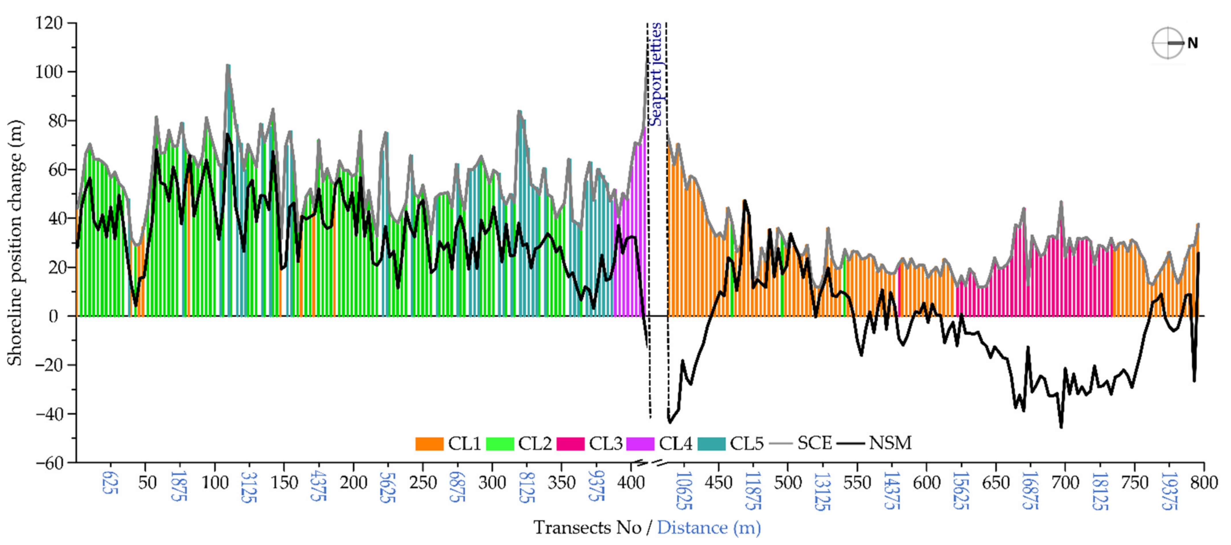
| Clusters | Transects | SCE (m) | NSM (m) | ||||
|---|---|---|---|---|---|---|---|
| No. | No. | Mean | Min | Max | Mean | Min | Max |
| 1 | 285 | 29.34 ± 1.38 | 11.8 | 70.36 | 4.07 ± 2.07 | −43.49 | 65.62 |
| 2 | 255 | 55.74 ± 1.44 | 27.29 | 92.43 | 38.93 ± 1.53 | 4.3 | 69.97 |
| 3 | 117 | 25.41 ± 1.41 | 11.92 | 46.76 | −22.70 ± 1.74 | −45.53 | 0.7 |
| 4 | 27 | 64.25 ± 6.91 | 40.51 | 108.85 | 20.74 ± 5.52 | −11.66 | 37.07 |
| 5 | 114 | 62.68 ± 2.18 | 38.01 | 102.62 | 27.66 ± 2.17 | 3.13 | 74.44 |
Publisher’s Note: MDPI stays neutral with regard to jurisdictional claims in published maps and institutional affiliations. |
© 2021 by the authors. Licensee MDPI, Basel, Switzerland. This article is an open access article distributed under the terms and conditions of the Creative Commons Attribution (CC BY) license (https://creativecommons.org/licenses/by/4.0/).
Share and Cite
Kondrat, V.; Šakurova, I.; Baltranaitė, E.; Kelpšaitė-Rimkienė, L. Natural and Anthropogenic Factors Shaping the Shoreline of Klaipėda, Lithuania. J. Mar. Sci. Eng. 2021, 9, 1456. https://doi.org/10.3390/jmse9121456
Kondrat V, Šakurova I, Baltranaitė E, Kelpšaitė-Rimkienė L. Natural and Anthropogenic Factors Shaping the Shoreline of Klaipėda, Lithuania. Journal of Marine Science and Engineering. 2021; 9(12):1456. https://doi.org/10.3390/jmse9121456
Chicago/Turabian StyleKondrat, Vitalijus, Ilona Šakurova, Eglė Baltranaitė, and Loreta Kelpšaitė-Rimkienė. 2021. "Natural and Anthropogenic Factors Shaping the Shoreline of Klaipėda, Lithuania" Journal of Marine Science and Engineering 9, no. 12: 1456. https://doi.org/10.3390/jmse9121456
APA StyleKondrat, V., Šakurova, I., Baltranaitė, E., & Kelpšaitė-Rimkienė, L. (2021). Natural and Anthropogenic Factors Shaping the Shoreline of Klaipėda, Lithuania. Journal of Marine Science and Engineering, 9(12), 1456. https://doi.org/10.3390/jmse9121456