Article

Relationship of Spatial Phytoplankton Variability during Spring with Eutrophic Inshore and Oligotrophic Offshore Waters in the East Sea, Including Dokdo, Korea

1
Risk Assessment Research Center, Korea Institute of Ocean Science and Technology, Geoje 53201, Korea
2
Ulleungdo Dokdo Ocean Science Station, Korea Institute of Ocean Science and Technology, Ulleung 40205, Korea
3
Dokdo Research Center, Korea Institute of Ocean Science and Technology, Uljin 36315, Korea
*
Author to whom correspondence should be addressed.
J. Mar. Sci. Eng. 2021, 9(12), 1455; https://doi.org/10.3390/jmse9121455
Submission received: 11 November 2021 / Revised: 18 December 2021 / Accepted: 19 December 2021 / Published: 20 December 2021

Abstract

:
The area near the subpolar front of the East Sea has high primary productivity during the spring season. We conducted two surveys, one in early spring and another in late spring, to assess environmental factors that influence phytoplankton community structure during these times. During early spring, vertical mixing supplied abundant nutrients to the surface. Due to the well-mixed water column, there were high nutrient levels, but total phytoplankton abundances and diversity were relatively low and were dominated by the diatom Chaetoceros spp. During late spring, the water column gradually stratified, with relatively high levels of nutrients in the surface layers near the coastal areas. Phytoplankton abundance and diversity at that time were higher, and there were diatoms (Pseudo-nitzschia spp. and Chaetoceros spp.), cryptophytes, and small flagellates. Pseudo-nitzschia spp. were especially abundant in re-sampled areas. The presence of a stratified and stable water mass and sufficient nitrate led to high phytoplankton growth, even in the open sea during late spring. These findings provide a better understanding of how phytoplankton population dynamics in the East Sea depend on water column stability during both early and late spring seasons.

1. Introduction

Phytoplankton are a foundational part of marine ecosystems and have a significant effect on overall ecological community dynamics. Many oceanographic features, such as temperature, salinity, and nutrient availability, influence the timing and distribution of phytoplankton blooms. An influx of coastal nutrients can also trigger phytoplankton blooms and species succession [1,2]. Offshore waters and most open-shelf waters have relatively low nutrient concentrations. The dominance of phytoplankton in these areas strongly depends on the supply of extraneous nutrients and cell accumulation by water currents. As a result, the coastal, pelagic, and estuarine zones may differ in nutrient concentrations, phytoplankton species, and total species abundance. Many studies throughout the world have documented this general pattern of a nutrient gradient and its impact on phytoplankton communities and primary production [3,4].
The East Sea (also called the Sea of Japan) is a marginal, semi-closed area of the ocean that is in the northwestern Pacific, between the Eurasian continent and Japan and has an average water depth of 1700 m. Isobe and Isoda [5] and Isoda and Saitoh [6] demonstrated that the East Sea had a well-defined subpolar front at a latitude of approximately 37 to 40° N. At this front, there is a meeting of the East Korea Warm Current (EKWC), which branches from the Tsushima Warm Current (TWC) through the Korean Strait (KS), and the North Korea Cold Current (NKCC) (Figure 1a). The TWC flows into the East Sea through the KS and exits through the Tsugaru and Soya straits. According to Gong and Son [7] and Martin and Kawase [8], the northern region of the East Sea is cooler, has a salinity of approximately 34.0, is nutrient-rich, and has a high oxygen content. In contrast, the southern region of the East Sea (i.e., Ulleung Basin) is warmer, slightly more saline (approximately 34.5), and nutrient-poor. These dynamic hydrological features, along with upwelling, eddies, and winds, create a unique environment that has high biological productivity and supports many marine fisheries [9,10,11,12,13,14].
The Ulleung Basin is heavily influenced by wind patterns and mixing during winter and spring [15]. Episodic windstorms at that time can significantly alter these aquatic ecosystems [16,17,18], and the increased levels of nutrients provided by these winds can promote phytoplankton blooms during spring. During the winter, phytoplankton biomass is typically low and evenly distributed throughout the water column [19,20,21].
However, our previous study [22] reported that during spring 2016, the episodic southerly windstorms increased Ekman transport eastward causing increased upwelling and the inflow of nutrients to the surface; this triggers phytoplankton blooms, especially in the vicinity of Ulleungdo and Dokdo with a time lag. This phenomenon is known as the “island effect”. This time lag between wind and chlorophyll increases has also been well demonstrated by satellite surveys. According to Kim et al. [23], spring blooms began 6∼15 days after wind stress weakened. On the other hand, Lee et al. [24] demonstrated that strong northwest winds suppressed upwelling, prevented nutrients from reaching the surface layer and led to low overall phytoplankton biomass during the spring of 2017. Therefore, wind speed and direction greatly influence the generation and extinction of phytoplankton blooms in the Ulleung Basin and the southeastern Korean coast of the East Sea.
Another feature that maintains phytoplankton biomass in this region is the transport of eutrophic water from the southern coast to the Ulleung Basin by currents and the Ulleung Warm Eddy (UWE) [13,25,26,27]. The waters of the southern coast of Korea are highly eutrophic due to the influx of nutrients from several rivers (Nakdong, Taehwa, Hyungsan), especially during the winter [28]. Moreover, Ahn et al. [29] and Kim et al. [30] reported a large-scale transport of algal blooms from the southern Korean coastal waters based on satellite imaging of chlorophyll a (Chl a). This indicates that most phytoplankton from the Southern Korean coastal waters can be transported into the East Sea, especially when other factors are present, such as the flow of the TWC and UWE.
Because these processes in the East Sea and Ulleung Basin are dynamic, continuous monitoring is needed to better understand inter-annual variations. It is particularly important to understand how water column stability affects phytoplankton distribution. We, therefore, conducted two surveys, one in early spring and another in late spring, to establish baseline trends and determine zonal differences in ocean conditions and phytoplankton assemblages. Based on the aforementioned studies in this area, we expect that as spring progresses, the water column will become more stratified as the winds decrease. Additionally, this study was conducted to determine how phytoplankton respond after the wind that causes mixing and change of water stability. Our purpose was to characterize changes in the horizontal distribution of phytoplankton in early and late spring according to the zones of the East Sea and to report the changes in phytoplankton after the time lag during the same survey period. This study on the ecology of primary producers will be helpful to explain how the East Sea maintains high fishery productivity despite being oligotrophic.

2. Materials and Methods

2.1. Cruise Information

The early spring survey covered the area from the southern coast of Korea to Dokdo around the Ulleung Basin, also known as the Busan-Ulleungdo-Dokdo line, during 2018 while onboard the R/V Eardo from 27 February to 5 March (Stns. 1–19; Figure 1). The late spring survey covered the area from the eastern coast of Korea to Dokdo, also known as the Uljin-Ulleungdo-Dokdo line, during 2018 while onboard the R/V Jangmok II from 2 June to 7 June (Stns. 20–47).

2.2. Survey Stations and Zones

Based on previous oceanic and geographical results [23,26], we distinguished three zones for each survey. For the early spring survey (Figure 1b), samples were from 19 stations that ranged from the southern coast of South Korea to Dokdo. The coastal stations (CS, Stns. 1–3) were in a coastal area where upwelling occurs frequently and is influenced by the Nakdong River, which provides freshwater input and nutrient pulses. The open-ocean stations (OS, Stns. 4, 5, 8–11, and 16–19) were in open offshore waters. The island stations (IS) were near Ulleungdo (Stns. 6–7) and Dokdo (Stns. 12–15) (Figure 1b). For the late spring survey (Figure 1c), samples were from 28 stations in three zones: the Uljin-Ulleungdo area from coast to open ocean (UU, Stns. 20–32); the vicinity of Ulleungdo and Dokdo (UL, Stns. 33–39, 46, and 47) known to have an island effect; and the area between Ulleungdo and Dokdo which remains oligotrophic (UD, Stns. 40–45). Samples from some stations were also collected on the return trip to determine if there was a change in phytoplankton abundance over time. The resampled sites were labeled with an “a” meaning “after time lag”. Those were Stns. 1a, 2a, 3a, 4a, 6a, 10a during early spring, and Stns. 21a–32a during late spring.

2.3. Hydrological Data

For the horizontal profiles, water temperature, salinity, and dissolved oxygen at the surface were measured using a YSI 6600 data sonde (USA). Surface water was collected using a bucket at all sampling stations during both sampling times. The vertical profiles of temperature, salinity, oxygen, and fluorescence were measured using a conductivity, temperature, and depth (CTD) sensor (SBE 911 plus CTD; 330., Bellevue, WA, USA) that was mounted on a rosette sampler of each ship at some stations (Stns. 3, 4, 10, 40, 42, 44, 3a, 4a, 10a, 22a, 26a, 30a). Surface salinity and temperature along the cruise track were continuously recorded using a thermosalinograph (TSG; SBE21, SeaBird Inc., Bellevue, WA, USA). All tracks of the early spring survey were recorded (Figure 2a). During the late spring survey, records began from Ulleungdo (3 June). We made several trips in the area between Ulleungdo and Dokdo and were able to obtain repeated daily TSG data (3–6 June) (Figure 2a).

2.4. Chlorophyll a and Nutrients

For measurements of nutrients and Chl a, water samples were passed through a glass microfiber filter (GF/F; Whatman, Middlesex, U.K.), and then placed in acid-cleaned polyethylene bottles. The filters for Chl a and water samples that were fixed with HgCl2 [31] for nutrient analysis were stored at −20 °C until subsequent analysis. In the laboratory, the ammonium, nitrate, nitrite, phosphate, and silicate concentrations were determined using a flow injection auto-analyzer (QuikChem 8000; Lachat Instruments, Loveland, CO, USA). Nutrient concentrations were calibrated using standard brine solutions (CSK Standard Solutions; Wako Pure Chemical Industries, Osaka, Japan). Chl a measurements were performed by extraction of the filtered material with 90% acetone in the dark for 24 h, followed by measurements using a Turner Design fluorometer (10-AU; Turner BioSystems, Sunnyvale, CA, USA). Chl a concentration (µg L−1) was calculated from fluorescence.

2.5. Phytoplankton Community

To identify and enumerate phytoplankton, subsamples (500 mL) were stored after fixation with 0.5% Lugol’s solution in polyethylene bottles. These subsamples were concentrated to approximately 10 to 50 mL by decanting the supernatant [32]. A Sedgewick-Rafter counting chamber was used to estimate the number of phytoplankton using light microscopy.

2.6. Meteorological Data

A time series of data from the Ulleungdo Ocean Data Buoy (Korea Meteorological Administration) was also assessed. This buoy measures air pressure, maximum wave height, wind gust speed, and wind direction at 1 h intervals. All data reported in this study were from the sampling periods of early spring (20 February to 15 March) and late spring (20 May to 10 June).

2.7. Statistical Analysis

Statistical differences in abiotic and biotic factors in the CS, OS, and IS zones (early spring) and in UU, UL, and UD zones (late spring) were assessed using an analysis of variance (ANOVA) followed by a Tukey’s test. A t-test was used to compare the means of variables at resampled stations before and after a time lag. A difference was considered significant when the p-value was less than 0.05. All statistical analyses were performed using SPSS version 17.0 (SPSS, Inc., Chicago, IL, USA). The impacts of measured environmental factors on the occurrences of dominant phytoplankton were determined by canonical correspondence analysis (CCA) using CANOCO version 4.5 for Windows.

3. Results

3.1. Distribution of Surface Temperature and Salinity

Our measurements from an on-ship TSG indicated the sea surface temperature (SST) ranged from 7 to 15 °C during early spring (Figure 2a) and 15 to 21 °C during late spring (Figure 2b).
There were clear temperature differences among stations during the early spring survey (Figure 2a). In particular, the waters surrounding the inner Jinhae Bay to the Nakdong River Estuary (Stn. 1) ranged from 7 to 9 °C, the Busan coast and Pohang offshore area (the region most influenced by the TWC, Stns. 2–4) ranged from 12 to 15 °C, and regions near Ulleungdo and Dokdo (Stns. 6–16) ranged from 9 to 12 °C. During the late spring survey, overall temperatures were 6 to 8 °C warmer than from the early spring survey (Figure 2b). There was also distinct temperature variations in the late spring survey. The inshore waters off the coast of Uljin were about 15 °C, the Uljin offshore-Ulleungdo line ranged from 17 to 19 °C, the waters around Ulleungdo ranged from 15 to 20 °C, and the Ulleungdo-Dokdo line ranged from 18 to 20 °C. Specifically, on the 3 June, cold water of 15 °C was observed on the east coast of Ulleungdo, which persisted to the following two days. From 5 June, the water temperature rose approximately 5 °C.
Our sonde-based measurements of the horizontal distribution across all stations indicated similar trends as the onboard TSG sensor. The sonde data indicated the SST ranged from 6.66 to 13.87 °C, with an average of 9.54 ± 1.53 °C during early spring (Figure 3a), although there were no significant differences in SST among zones (Table 1). During late spring, water temperature ranged from 15.29 to 20.21 °C, with an average of 18.47 ± 1.00 °C (Figure 3b), similar to the early spring mean temperatures; there were also no significant differences in SST among zones. Thus, geographical variations of SST were greater during early spring than late spring.
Overall salinity during late spring was lower than during early spring (Figure 3). The surface salinity varied from 33.58 to 34.86, with an average of 34.48 ± 0.24 during early spring, and salinity was not significantly different among zones (Table 1). During late spring, the salinity varied from 34.09 to 34.52, with an average of 34.36 ± 0.15. ANOVA indicated a significant difference among zones, with the UU zone (average: 34.27 ± 0.09) and UL zone (average: 34.33 ± 0.21) significantly different from the UD zone (average: 34.46 ± 0.04; p < 0.05, F-value: 3.720).

3.2. Meteorological Features

During the early spring survey, there were strong winds, and on 28 February a strong wind episode associated with low air pressure (988 hPa) passed through the Ulleung Basin. The wind direction shifted from the southeast to a strong wind from the northwest. At that time, the waves around Ulleungdo and Dokdo reached a height of 9.4 m and the wind speed was 24.8 m s−1 (Figure 4a). During the late spring sampling time (2 to 7 June) there were no specific wind episodes associated with low pressure and no high wind speeds, although there were constant southerly winds (Figure 4b).

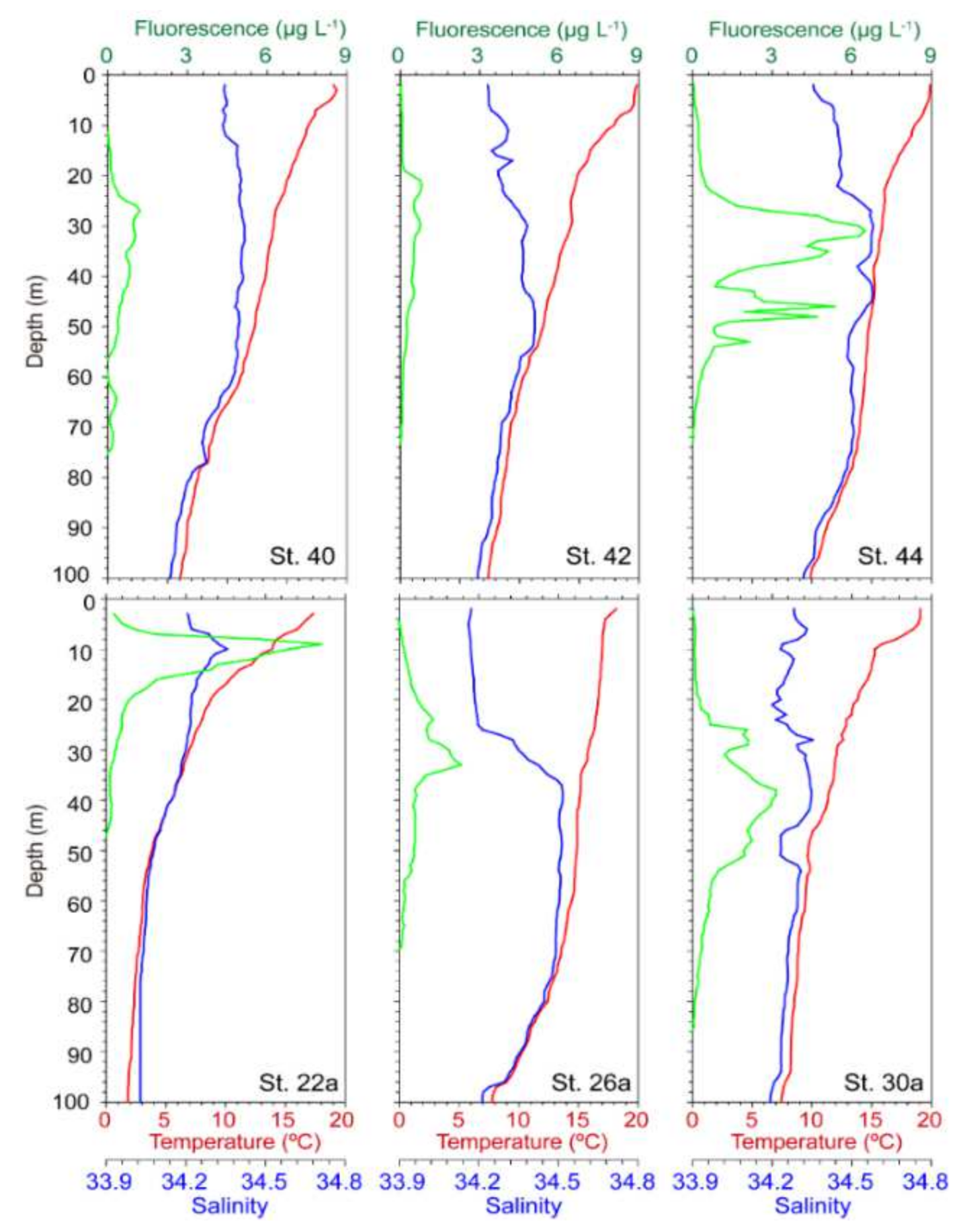
3.3. Vertical Profiles

Our data on the vertical profiles of selected inshore and offshore stations indicated that salinity and temperature remained relatively constant in the upper 60 m of the water column during early spring (Figure 5). The thermocline began at a depth of less than 80 m at Stn. 4. In the resampled results of Stns. 3a, 4a, and 10a, a weaker stratified layer was formed than in previous studies, but there was still a small difference in water temperature between the surface and at depth. A subsurface chlorophyll maximum (SCM) was not observed during the early spring period, and the surface water mass was mostly mixed. The level of fluorescence was relatively low and relatively constant.
In contrast, during late spring, the vertical profiles of selected offshore and near-island stations had more stratification of temperature, salinity, and fluorescence in the water column (Figure 6). In particular, evidence of water temperature stratification is clearly present in the late spring (Figure 6). An SCM layer was present in the thermocline layer with a strong difference in density. Water stratification was more evident in the vertical profiles on the later sampling dates (Stns. 22a, 26a, and 30a), with temperatures in the upper 10 to 15 m ranging from 15 to 20 °C. The temperature was lower than 10 °C at depths below 50 m at Stns. 22a, 30a, and at depths below 80 m at Stn. 26a. The Chl a levels were much more variable and had sharper increases (up to almost 9 µg L−1 at Stn. 22a) during late spring.

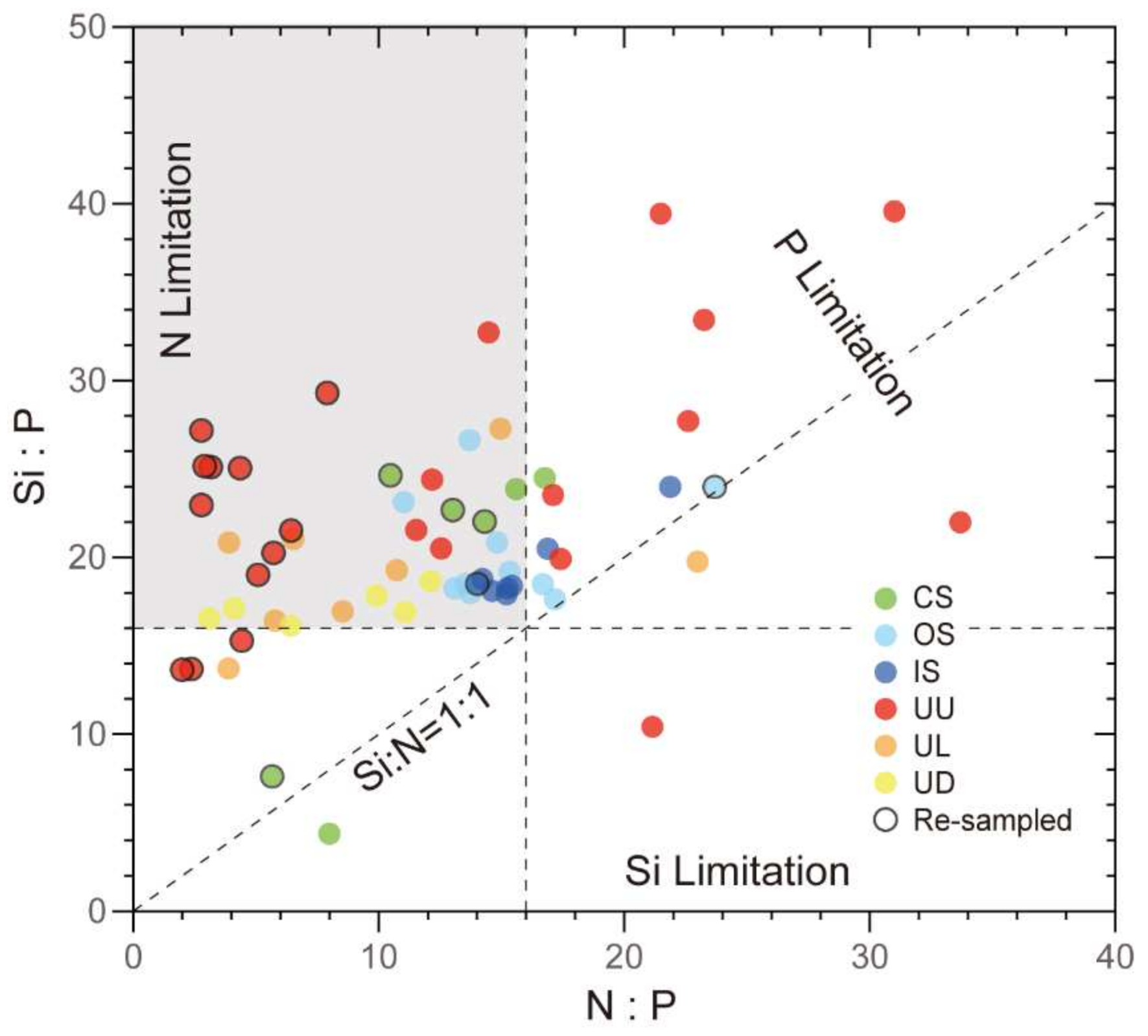
3.4. Distribution of Nutrients
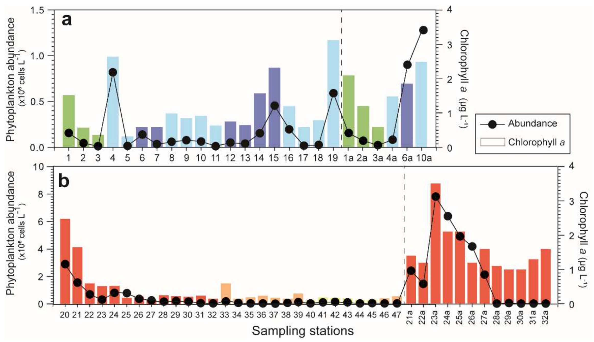
Dissolved inorganic nutrients had large spatial variations during early spring (Figure 7), but the different zones were not significantly different (Table 1). At that time, the nitrate + nitrite level ranged from 0.70 to 6.70 µM (average: 5.01 ± 1.58 μM) and was relatively high at most stations, except Stn. 1. The ammonium level ranged from 0.04 to 2.10 µM (average: 0.71 ± 0.52 µM) and the level varied greatly among stations. The phosphate level was high, ranging from 0.19 to 0.45 µM (average: 0.38 ± 0.07 μM), had relatively little variation among stations, and had similar trends as the changes in nitrate + nitrite. The silicate concentration was also high, except at Stn. 1, and varied from 0.82 to 10.93 µM (average: 7.61 ± 2.23 µM). There was no significant difference over time (Table 2; p > 0.05, t-test).
During late spring, the nutrients had small spatial variations; they were highest at stations closest to the coast (Stns. 20–35) and were lower in offshore regions (UU and UL zones; Figure 8). However, there were no significant differences among the zones (Table 1). The nitrate + nitrite level ranged from 0.30 to 5.05 µM (average: 1.13 ± 1.01 μM). The ammonium level was relatively high and ranged from 0.03 to 7.14 µM (average: 0.52 ± 1.11 µM). The phosphate level ranged from 0.05 to 0.57 µM (average: 0.15 ± 0.08 μM), and low levels were in response to phytoplankton. The silicate concentration varied from 1.58 to 7.96 µM (average: 3.28 ± 1.33 µM; Figure 8). After the time delay, the nitrate + nitrite concentration in the UU zone was significantly lowered from 1.61 ± 1.08 to 0.52 ± 0.19 on average (Table 2; p < 0.01, t-value = 3.592).

3.5. Chlorophyll a

The early and late spring surveys had no differences in surface Chl a concentrations among zones. In the early spring survey, the surface Chl a concentration ranged from 0.00 to 3.12 µg L−1 (average: 1.20 ± 0.81 µg L−1). The spatial variation in Chl a was relatively large, and high concentrations were between Stn. 4 (2.64 µg L−1 on 27 February) and Stn. 19 (3.12 µg L−1 on 5 March), which are located near the TWC. The level of Chl a was low (<1.0 µg L−1) between Ulleungdo and Dokdo (Stns. 6–13) (Figure 9a). For the late spring survey, the Chl a concentration varied from 0.40 to 3.50 µg L−1 (average: 1.32 ± 0.65 µg L−1). The Chl a level was high at Stn. 20 on June 2 and low between Stns. 37 and 47 from 3 to 6 June. When there was a 6-day time lag in sampling, the Chl a concentration between Stn. 23a and 27a increased by about 5-fold at Stn. 23a and by about 3-fold at Stn. 27a. These two stations are located near the TWC, and similar to stations of the early spring survey. Overall, the level of Chl a and the abundance of phytoplankton had similar changes over time (Figure 9b).

3.6. Phytoplankton Abundance

We measured the total abundance of phytoplankton at each station during early spring and late spring (Figure 9). During early spring, the total phytoplankton abundance ranged from 9.70 × 10³ to 1.28 × 10⁶ cells L−1 (average: 2.20 × 10⁵ ± 3.32 × 10⁵ cells L−1). During late spring, the total phytoplankton abundance ranged from 1.45 × 10⁴ to 7.80 × 10⁶ cells L−1 (average: 9.82 × 10⁵ ± 1.85 × 10⁶ cells L−1). There were no significant differences in overall phytoplankton abundance among zones during early spring. However, during late spring, the phytoplankton abundance in zone UU was about seven times higher than in the other zones (p < 0.05, F-value = 3.834, ANOVA). In particular, zone UU had an average abundance of 7.17 ± 9.28 × 10⁵ cells L−1, much greater than in zone UL (0.42 ± 0.80 × 10⁵ cells L−1) and zone UD (0.43 ± 0.18 × 10⁵ cell L−1) (Table 1). Phytoplankton abundance increased significantly with a time lag during early spring (p < 0.05, t-value = −0.746) and late spring (p < 0.05, t-value = 2.69) (Table 2). During early spring, the phytoplankton abundance increased from 2.05 ± 3.05 × 10⁵ to 4.18 ± 5.35 × 10⁵ cells L−1; during late spring the phytoplankton abundance increased approximately fivefold, from 5.11 ± 5.85 × 10⁵ to 24.44 ± 27.57 × 10⁵ cells L−1.

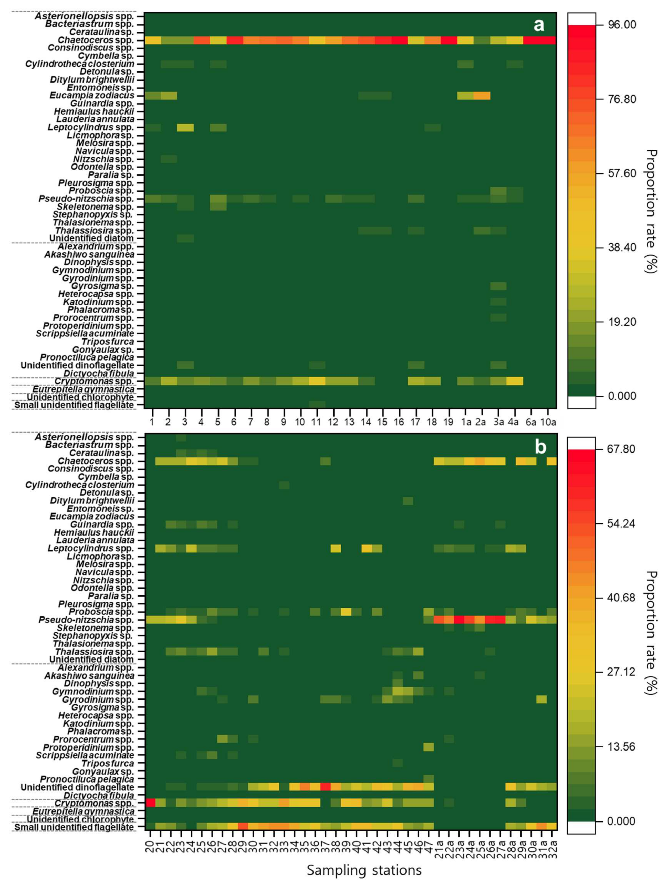
3.7. Phytoplankton Community

We also examined the proportions of different phytoplankton species at the different stations during early spring and late spring (Figure 10). During early spring, Chaetoceros spp. accounted for ~80% of all species for all stations together. There were relatively high proportions (~60%) of Eucampia zodiacus at Stn. 2a, and cryptophytes at Stns. 11 and 4a (Figure 10a). Overall, there were more species during the late spring survey. Diatoms were the dominant phytoplankton group with Pseudo-nitzschia spp. (~55%) at Stns. 20 to 24 and 20a to 26a, Chaetoceros spp. (~30%) at Stns. 21 to 28 and 21a to 32a, and Leptocylindrus danicus (25%) at Stn. 42. The other common groups were various dinoflagellates (~53%) at Stns. 32 to 46, cryptophytes (~41%) at Stns. 20 and 29 to 36, and unidentified small flagellates (~48%) at Stns. 28 to 35 and 29a to 32a (Figure 10b).

3.8. Comparison of Environment in Early Spring and Late Spring

In order to compare the marine environment in early spring and late spring, stations between Ulleungdo and Dokdo overlapping regions (Stns. 6–13 vs. Stns. 19–28) were compared (Table 3). In late spring, the water temperature was about 10 °C higher than in early spring (p < 0.001, t-value = −13.40). Dissolved oxygen was high in early spring when the water temperature was low (p < 0.001, t-value = 12.14). All nutrients were clearly high in early spring (p < 0.05). In particular, nitrate showed the greatest difference with an average of 6.17 ± 0.43 μM and 0.8 ± 0.48 μM (p < 0.001, t-value = 19.84). Chl. a was somewhat higher in early spring (p < 0.01, t-value = 4.329), but there was no significant difference in phytoplankton abundance (p > 0.05). The composition of phytoplankton was clearly high in diatoms in early spring (p < 0.05, t-value = 3.196), and relatively high in dinoflagellates (p < 0.001, t-value = −5.684) and other algae (p < 0.001, t-value = 12.14) in late spring.

3.9. Canonical Correspondence Analysis

We performed a canonical correspondence analysis (CCA) to determine the relationships of the most dominant species with different environmental variables during early spring and late spring (Figure 11).
The CCA results indicated that variables such as temperature, dissolved oxygen (DO), ammonium (NH4), nitrate + nitrite (NO2 + NO3), salinity, pH, Chl a, dissolved silicate (DSi), and dissolved inorganic phosphate (DIP) can explain the variability of phytoplankton species. In particular, during early spring, Eucampia zodiacus and Pseudo-nitzschia spp. had negative correlations with nitrate + nitrite, DIP, and Dsi (all p < 0.05). Each dominant phytoplankton species had a significant correlation with Chl a (all p < 0.05), and Chaetoceros spp. had the strongest relationship with Chl a (p < 0.01) (Figure 11a). During late spring, most of the nutrients (nitrate + nitrite, ammonium, and DIP) had negative correlations with pH, DO, and salinity (all p < 0.05). Moreover, most of the initially sampled stations had negative correlations with Chl a, but the resampled stations had positive correlations with Chl a (Figure 11b).

4. Discussion

4.1. Environmental Characteristics and Phytoplankton Dynamics during Early Spring

We assessed surface water temperature gradients during early spring using SST data from an onboard TSG sensor (Figure 2). These data clearly distinguished waters influenced by the EKWC and southeastern Korean coastal waters, implying that the warm water from the TWC and EKWC had a great influence on the East Sea, particularly in the Ulsan and Pohang offshore waters, the region included in our CS zone. Baek et al. [33] described a similar thermal front between the EKWC and the Nakdong Estuary in Busan coastal waters. The TWC flows into the East Sea through the KS, which has warm and more saline water (~34.5).
Our results indicated that episodic winds during early spring maintained a relatively well mixed water column to a depth of about 60–80m (Figure 5). Among them, the water layer up to 100 m was clearly mixed at Stn. 10, and this is a typical mixed water mass in the East Sea in winter [28]. In particular, a strong windstorm passed the Ulleung Basin on 28 February, and the southeast winds changed into strong northwest winds. Episodic windstorms play an important role in mixing the water column and supplying nutrients to the surface layer [34,35]. As a result, during early spring nutrient concentrations were relatively high at all stations, including the open sea, regardless of the distribution of phytoplankton, and the differences in nutrients among zones were insignificant.
The ratio between nutrients (N/P/Si) in early spring is distributed in a relatively even Redfield ratio (Figure 12). Although the N/P ratio was slightly lower than 16, there was no evidence of nutrient limitation because the absolute concentration of the nutrient was sufficient. Despite the high nutrient supply, phytoplankton did not have significant proliferation due to the unstable water mass and relatively low water temperature. Only some diatoms dominated in certain patches.
The diatom Chaetoceros was the most dominant genus in almost all our stations (Figure 10a). The other major diatoms were Eucampia zodiacus, Thalassiosira spp., and Pseudo-nitzschia spp. Despite high levels of nutrients, such nitrate + nitrite and silicate, the overall abundance of phytoplankton was relatively low. Our CCA results confirmed this result, in that E. zodiacus, and Pseudo-nitzschia spp. had significant negative correlations with nitrates + nitrites, DIP, and DSi (all p < 0.01, Pearson’s correlation; Figure 11a). A possible reason for the low abundances of phytoplankton despite atypically high nutrient levels is that there was a delay between the influx of nutrients and phytoplankton blooms. It is fairly common in the East Sea for phytoplankton to bloom three to five days after a windstorm, once the water mass has stabilized [23]. This was confirmed by our resampling data, which indicated that phytoplankton abundance increased from 2.05 ± 3.05 × 10⁵ to 4.18 ± 5.35 × 10⁵ cells L−1. In the resampled vertical profile, the increase in abundance was only modest at Stns. 3a and 4a but are stratified more than in the previous investigation (Figure 5).
An undeveloped phytoplankton community with low abundance and diversity is common in well-mixed and nutrient-rich waters during early spring. During the early spring, Chaetoceros spp. were mainly C. socialis, which we observed when silicate levels were high. Because the water column was well mixed, DSi from the bottom layers was introduced to the surface. In contrast, during spring 2017 suppression of upwelling kept most of the DSi below 100 m [24]. In the East Sea, C. socialis appears during the winter when waters are relatively cooler, but this species also occurs in the warm waters of the Mediterranean Sea and the Gulf of California [36]. Recent reports described pseudocryptic diversity within the C. socialis complex. It is, therefore, uncertain if C. socialis is a eurythermal species or if different strains of C. socialis have different thermal tolerances [37,38]. This species is present year-round off the coast of Korea but is most dominant in the East Sea and the coast of Jeju when water temperatures are low [39,40]. This suggests the C. socialis in this region could be a strain that is tolerant of low temperatures [41].
The diatom E. zodiacus had a relatively high abundance at the inshore area of CS, which is cold. Nishikawa et al. [42] reported that E. zodiacus usually occurred throughout the year in temperate waters and was most abundant between February and April. Baek et al. [21,28] reported that E. zodiacus was mainly dominant during winter in the cold water at the southern Korean coast, similar to the results in the present study. This indicated that water at a low temperature is more likely to support E. zodiacus. Overall, although high nutrient levels were related to water column mixing, phytoplankton did not develop even in the presence of abundant nutrients, except for the genera Chaetoceros and Eucampia.

4.2. Environmental Characteristics and Phytoplankton Dynamics during Late Spring

The overall environmental conditions during the late spring were more stable, and there were no episodic windstorm events (Figure 4b). As the winds weaken and solar radiation increases during spring, this increases the stratification of the water column. The combination of a warm, stratified water column with sufficient nutrients during late spring leads to a rapid increase in phytoplankton [43,44]. We observed relatively high levels of nitrate + nitrite and silicate along the coastal waters and in some areas of Ulleungdo during late spring. However, there are still various interpretations regarding the supply of nutrients to the offshore area of the East Sea [13,45,46,47].
In terms of nutrient ratios, most areas were more nitrate-depleted than in early spring (Figure 12). The N/P ratio for the entire East Sea is in the range of 11.4 to 14.70, significantly lower than the Redfield ratio of 16, and the most reported N/P ratio for the East Sea is 12.7 ± 0.1 [16,48]. As such, nitrate is the growth-limiting nutrient for phytoplankton growth in the East Sea. However, for the reasons mentioned above, nutrients can be supplied to the East Sea from several sources, and water high in nitrate is mainly from the coastal regions [13,45]. However, in the UU zone, nitrate + nitrite was higher than the absolute concentration of 1µM, which is the amount where phytoplankton growth was inhibited. In addition, silicates were abundant at most times and in most regions, thus providing a favorable environment for diatoms to dominate when there are adequate levels of other nutrients. When the phytoplankton proliferated, the nutrient ratios shifted to indicate strong nitrate limitation.
It is well known that discharges from major rivers, such as the Nakdong River in Busan, the Taehwa River in Ulsan, and the Hyungsan River in Pohang, provide nutrients to the East Sea, particularly during the rainy seasons (spring and summer). Satellite data indicated that these nutrients and the associated phytoplankton communities were transported by the EKWC to oligotrophic off-shore areas and the open ocean [29,30]. The anticyclonic Ulleung Warm Eddy (UWE), a branch of the EKWC, is another method of transport in the East Sea. There is evidence that this eddy introduces productive coastal waters and transports micro-organisms into the central Ulleung Basin [4]. However, these data only suggest various possibilities of transport, and it is premature to provide a definitive conclusion regarding the actual mechanism.
The episodic high-wind event and the associated increase of biomass that we recorded was a notable observation. Volcanic islands, such as Ulleungdo and Dokdo, with an average surrounding water depth of 1700 m, can contribute to an “island effect” [27]. These events are important in determining the spring development of phytoplankton biomass. The leeward sides of islands tend to have lower water temperatures and higher levels of nutrients [49,50,51]. During our late spring survey, we measured the coastal SST of Ulleungdo daily using the TSG that was installed on the ship (Figure 2b). There was evidence of anomalously cooler water (~15–17 °C) during the late spring survey of SST at stations leeward of Ulleungdo, and these temperatures recovered over the next 3 days to a more typical range of ~18.5 to 19.5 °C. Additionally, nitrate + nitrite and silicate concentrations were somewhat higher than in areas windward of Ulleungdo. This is one of the many factors that supply nutrients to the East Sea, which is known to be oligotrophic. The sudden introduction of low temperature water and nutrients near the coast of Ulleungdo supported a high phytoplankton abundance, which can benefit the ecosystem of these oligotrophic waters and are critical to high-trophic organisms [52].
The dominant species among stations during late spring included Chaetoceros spp., Pseudo-nitzschia spp., and cryptophytes, with low-to-moderate amounts of various dinoflagellates. In zone UU, there were high proportions of Chaetoceros spp., with some Pseudo-nitzschia spp. Along the UD and UL lines, there were high proportions of unidentified dinoflagellates and cryptophytes, but the total phytoplankton abundance was low at that time, so these high proportions are not particularly meaningful. There was a significantly greater abundance (~7-fold) of phytoplankton in the UU than in the UL and UD. This was unsurprising, because the UU zone is on the continental shelf, and coastal zones are known to be eutrophic [53,54,55]. However, there was also a significant increase in phytoplankton biomass at resampling (5.11 ± 5.85 × 10⁵ cells L−1 vs. 24.44 ± 27.57 × 10⁵ cells L−1). Similar to the aforementioned phytoplankton dynamics during early spring, previous research reported a significant increase in phytoplankton abundance after the relaxation of winds [23] or upwelling [54]. Additionally, the influx of nutrients and organisms from coastal areas through the TWC can support the rapid growth of phytoplankton. In this area, the available nutrients were higher than the first sampling in the UU, and phytoplankton grew significantly by consuming these nutrients after a lag period. This is also supported by our CCA, in which the resampled stations became more positively correlated with Chl a (Figure 11b). In our first sampling, small cryptophytes with low nutrient consumption were dominant. It is likely that diatoms with an advantage in high-nutrient regions with a stable water mass were able to grow rapidly during the second sampling in the UU.
Our results indicated the resampled stations had overall higher abundances of phytoplankton, especially an increase of diatoms such as Pseudo-nitzschia spp., mainly P. delicatissima (Figure 10b). Pseudo-nitzschia spp. are common in Korean coastal waters. Some of these species are important because they are the only known diatoms to cause harmful algal blooms [56]. Due to the short lifespan of Pseudo-nitzschia spp., they tend to rapidly bloom and form large red tides when environmental conditions are favorable (warm water temperature and high availability of silicate and other nutrients) [57]. There is often a time lag, which allows stratification to increase and the water column to stabilize before the conditions are favorable for blooms [58]. In conclusion, nitrate is supplied to the East Sea in late spring for the same reasons as upwelling and mixing in the eastern coast of Korea. In addition, the stable water column was maintained due to the weather conditions in the late spring, which allowed for the rapid growth of genus Pseudo-nitzschia and the consumption of nutrients around the UU area for the following 7 days. A study of such rapid growth events of diatoms in spring in the East Sea, which is oligotrophic waters, will be important for understanding the mechanism of high-yielding fisheries in the East Sea.

5. Conclusions

In this study, we recorded data during two distinct phases—early spring and late spring. The early spring was characterized by strong winds and vertical mixing of the water column, which led to relatively high nutrient concentrations and an undeveloped phytoplankton community. On the other hand, the late spring was characterized by more abundant nutrients around the coastal areas than the offshore area and the maintenance of a stratified aquatic environment. Another characteristic of the late spring was the greater abundance of phytoplankton and the more complex phytoplankton community structure. Our re-sampling after a time delay indicated a rapid proliferation of diatoms. This confirmed that in the East Sea (which is usually in a nitrate-limited state) when a certain amount of nitrate combined with stable water conditions were combined, promoted the proliferation of phytoplankton with a time delay. Monitoring of these inter-annual changes is important for understanding the dynamic ecology of the Ulleung Basin and East Sea. Our results, which characterized the relationships of the distribution and growth of phytoplankton with changes in wind and stratification and in nutrient supply, provide an improved understanding of marine ecosystem dynamics in the East Sea.

Author Contributions

Conceptualization, S.-H.B. and M.L.; Sampling, M.L., Y.-B.K. and S.-H.B.; Formal Analysis, M.L.; Writing—Original Draft Preparation, M.L. and H.R.; Writing—Review & Editing, M.L. and H.R.; Visualization, M.L. and Y.-B.K.; Supervision, S.-H.B.; Project Management, C.-H.P.; Funding Acquisition, C.-H.P. All authors have read and agreed to the published version of the manuscript.

Funding

This work was supported by a project “a sustainable research and development of Dokdo (PG52260)” of the Ministry of Oceans and Fisheries and KIOST project “Biogeochemical cycling and marine environmental change studies” (PE99912).

Institutional Review Board Statement

Not applicable.

Informed Consent Statement

Not applicable.

Data Availability Statement

The data presented in this study are available on request from the corresponding author.

Acknowledgments

We would like to acknowledge the captains and crew onboard the R/V Eardo and R/V Jangmok II for making sampling possible.

Conflicts of Interest

The authors declare no conflict of interest.

References

  1. Lancelot, C.; Billen, G.; Sournia, A.; Weisse, T.; Colijn, F.; Veldhuis, M.J.W.; Davies, A.; Wassman, P. Phaeocystis Blooms and Nutrient Enrichment in the Continental Coastal Zones of the North Sea. Ambio 1987, 16, 38–46. [Google Scholar]
  2. Anderson, D.M.; Glibert, P.M.; Burkholder, J.M. Harmful algal blooms and eutrophication: Nutrient sources, composition, and consequences. Estuaries 2002, 25, 704–726. [Google Scholar] [CrossRef]
  3. Anderson, G.C.; Zeutschel, R.P. Release of dissolved organic matter by marine phytoplankton in coastal and offshore areas of the Northeast Pacific ocean. Limnol. Oceanogr. 1970, 15, 402–407. [Google Scholar] [CrossRef] [Green Version]
  4. Hyun, J.-H.; Kim, D.; Shin, C.-W.; Noh, J.-H.; Yang, E.-J.; Mok, J.-S.; Kim, S.-H.; Kim, H.-C.; Yoo, S. Enhanced phytoplankton and bacterioplankton production coupled to coastal upwelling and an anticyclonic eddy in the Ulleung basin, East Sea. Aquat. Microb. Ecol. 2009, 54, 45–54. [Google Scholar] [CrossRef]
  5. Isobe, A.; Isoda, Y. Circulation in the Japan Basin, the Northern Part of the Japan Sea. J. Oceanogr. 1997, 53, 373. [Google Scholar]
  6. Isoda, Y.; Saitoh, S. The northward intruding eddy along the East coast of Korea. J. Oceanogr. 1993, 49, 443–458. [Google Scholar] [CrossRef]
  7. Gong, Y.; Son, S. The study of the study on the marine thermo-front in the east sea of Korea. Rep. Nat. Fish. Res. Dep. Inst. 1982, 28, 24–25. [Google Scholar]
  8. Martin, S.; Kawase, M. The southern flux of sea ice in the Tatarskiy Strait, Japan Sea and the generation of the Liman Current. J. Mar. Res. 1998, 56, 141–155. [Google Scholar] [CrossRef]
  9. Chung, C.S.; Shim, J.H.; Park, Y.G.; Park, S.-G. Primary Productivity and Nitrogenous Nutrient Dynamics in the East Sea of Korea. J. Oceanol. Soc. Korea 1989, 24, 52–61. [Google Scholar]
  10. Moon, C.-H.; Yang, S.-R.; Yang, H.-S.; Cho, H.-J.; Lee, S.-Y.; Kim, S.-Y. Regeneration Processes of Nutrients in the Polar Front Area of the last Sea IV. Chlorophyll a Distribution, New Production and the Vertical Diffusion of Nitrate. Korean J. Fish. Aquat. Sci. 1998, 31, 259–266. [Google Scholar]
  11. Kwak, J.H.; Hwang, J.; Choy, E.J.; Park, H.J.; Kang, D.J.; Lee, T.; Chang, K.I.; Kim, K.R.; Kang, C.K. High primary productivity and f-ratio in summer in the Ulleung basin of the East/Japan Sea. Deep Sea Res. Part. I Oceanogr. Res. Pap. 2013, 79, 74–85. [Google Scholar] [CrossRef]
  12. Lee, J.Y.; Kang, D.J.; Kim, I.N.; Rho, T.; Lee, T.; Kang, C.K.; Kim, K.R. Spatial and temporal variability in the pelagic ecosystem of the East Sea (Sea of Japan): A review. J. Mar. Syst. 2009, 78, 288–300. [Google Scholar] [CrossRef]
  13. Yoo, S.; Park, J. Why is the southwest the most productive region of the East Sea/Sea of Japan? J. Mar. Syst. 2009, 78, 301–315. [Google Scholar] [CrossRef]
  14. Ji, R.; Jin, M.; Li, Y.; Kang, Y.H.; Kang, C.K. Variability of primary production among basins in the East/Japan Sea: Role of water column stability in modulating nutrient and light availability. Prog. Oceanogr. 2019, 178, 102173. [Google Scholar] [CrossRef]
  15. Lie, H.J.; Cho, C.H. Seasonal circulation patterns of the Yellow and East China Seas derived from satellite-tracked drifter trajectories and hydrographic observations. Prog. Oceanogr. 2016, 146, 121–141. [Google Scholar] [CrossRef]
  16. Ryan, J.P.; Polito, P.S.; Strutton, P.G.; Chavez, F.P. Unusual large-scale phytoplankton blooms in the equatorial Pacific. Prog. Oceanogr. 2002, 55, 263–285. [Google Scholar] [CrossRef]
  17. Zhao, H.; Tang, D.; Wang, Y. Comparison of phytoplankton blooms triggered by two typhoons with different intensities and translation speeds in the South China Sea. Mar. Ecol. Prog. Ser. 2008, 365, 57–65. [Google Scholar] [CrossRef] [Green Version]
  18. Tsuchiya, K.; Yoshiki, T.; Nakajima, R.; Miyaguchi, H.; Kuwahara, V.S.; Taguchi, S.; Kikuchi, T.; Toda, T. Typhoon-driven variations in primary production and phytoplankton assemblages in Sagami Bay, Japan: A case study of typhoon Mawar (T0511). Plankt. Benthos Res. 2013, 8, 74–87. [Google Scholar] [CrossRef] [Green Version]
  19. Smayda, T.J. Harmful algal blooms: Their ecophysiology and general relevance to phytoplankton blooms in the sea. Limnol. Oceanogr. 1997, 42, 1137–1153. [Google Scholar] [CrossRef]
  20. Baek, S.H.; Shimode, S.; Kim, H.C.; Han, M.S.; Kikuchi, T. Strong bottom–up effects on phytoplankton community caused by a rainfall during spring and summer in Sagami Bay, Japan. J. Mar. Syst. 2009, 75, 253–264. [Google Scholar] [CrossRef]
  21. Baek, S.H.; Kim, D.; Son, M.; Yun, S.M.; Kim, Y.O. Seasonal distribution of phytoplankton assemblages and nutrient-enriched bioassays as indicators of nutrient limitation of phytoplankton growth in Gwangyang Bay, Korea. Estuar. Coast. Shelf Sci. 2015, 163, 265–278. [Google Scholar] [CrossRef]
  22. Lee, M.; Kim, Y.-B.; Kang, J.H.; Park, C.H.; Baek, S.H. Seasonal phytoplankton dynamics in oligotriphic offshore water of Dokdo, 2018. Korean J. Environ. Biol. 2019, 37, 19–30. [Google Scholar] [CrossRef]
  23. Kim, H.C.; Yoo, S.; Oh, I.S. Relationship between phytoplankton bloom and wind stress in the sub-polar frontal area of the Japan/East Sea. J. Mar. Syst. 2007, 67, 205–216. [Google Scholar] [CrossRef]
  24. Lee, M.; Kim, J.H.; Kim, Y.-B.; Park, C.H.; Shin, K.; Baek, S.H. Specific oceanographic characteristics and phytoplankton responses influencing the primary production around the Ulleung Basin area in spring. Acta Oceanol. Sin. 2020, 39, 107–122. [Google Scholar] [CrossRef]
  25. Kang, Y.-S.; Choi, H.-C.; Lim, J.-H.; Jeon, I.-S.; Seo, J.-H. Dynamics of the Phytoplankton Community in the Coastal Waters of Chuksan Harbor, East Sea. Algae 2005, 20, 345–352. [Google Scholar] [CrossRef]
  26. Oh, H.J.; Suh, Y.S.; Heo, S. The Relationship Between Phytoplankton Distribution and Environmental Conditions of the Upwelling Cold Water in the Eastern Coast of the Korean Peninsula. J. Korean Assoc. Geogr. Inf. Stud. 2004, 7, 166–173. [Google Scholar]
  27. Baek, S.H.; Lee, M.; Kim, Y.B. Spring phytoplankton community response to an episodic windstorm event in oligotrophic waters offshore from the Ulleungdo and Dokdo islands, Korea. J. Sea Res. 2018, 132, 1–14. [Google Scholar] [CrossRef]
  28. Baek, S.H.; Lee, M.; Park, B.S.; Lim, Y.K. Variation in Phytoplankton Community Due to an Autumn Typhoon and Winter Water Turbulence in Southern Korean Coastal Waters. Sustainability 2020, 12, 2781. [Google Scholar] [CrossRef] [Green Version]
  29. Ahn, Y.-H.; Shanmugam, P.; Ryu, J.-H.; Jeong, J.-C. Satellite detection of harmful algal bloom occurrences in Korean waters. Harmful Algae 2006, 5, 213–231. [Google Scholar] [CrossRef]
  30. Kim, H.-C.; Yamaguchi, H.; Yoo, S.; Zhu, J.; Okamura, K.; Kiyomoto, Y.; Tanaka, K.; Kim, S.-W.; Park, T.; Oh, I.S.; et al. Distribution of Changjiang Diluted Water detected by satellite chlorophyll a and its interannual variation during 1998–2007. J. Oceanogr. 2009, 65, 129–135. [Google Scholar] [CrossRef]
  31. Parsons, T.R.; Maita, Y.; Lalli, C.M. A Manual of Chemical & Biological Methods for Seawater Analysis; Elsevier: Amsterdam, The Netherlands, 1984; ISBN 978-0-08-030287-4. [Google Scholar]
  32. Sournia, A. Phytoplankton Manual; United Nations Educational, Scientific and Cultural Organization: Paris, France, 1978; ISBN 92-3-101572-9. [Google Scholar]
  33. Baek, S.H.; Kim, D.; Kim, Y.O.; Son, M.; Kim, Y.J.; Lee, M.; Park, B.S. Seasonal changes in abiotic environmental conditions in the Busan coastal region (South Korea) due to the Nakdong River in 2013 and effect of these changes on phytoplankton communities. Cont. Shelf Res. 2019, 175, 116–126. [Google Scholar] [CrossRef]
  34. Chung, C.-C.; Gong, G.-C.; Hung, C.-C. Effect of Typhoon Morakot on microphytoplankton population dynamics in the subtropical Northwest Pacific. Mar. Ecol. Prog. Ser. 2012, 448, 39–49. [Google Scholar] [CrossRef] [Green Version]
  35. Tsuchiya, K.; Kuwahara, V.S.; Yoshiki, T.; Nakajima, R.; Miyaguchi, H.; Kumekawa, N.; Kikuchi, T.; Toda, T. Phytoplankton community response and succession in relation to typhoon passages in the coastal waters of Japan. J. Plankton Res. 2014, 36, 424–438. [Google Scholar] [CrossRef] [Green Version]
  36. Hasle, G.R.; Syvertsen, E. Marine Diatoms. In Identifying Marine Phytoplankton; Tomas, C.R., Ed.; Academic Press: San Diego, CA, USA, 1997; pp. 5–386. [Google Scholar]
  37. Degerlund, M.; Huseby, S.; Zingone, A.; Sarno, D.; Landfald, B. Functional diversity in cryptic species of Chaetoceros socialis Lauder (Bacillariophyceae). J. Plankton Res. 2012, 34, 416–431. [Google Scholar] [CrossRef] [Green Version]
  38. Gaonkar, C.C.; Kooistra, W.H.C.F.; Lange, C.B.; Montresor, M.; Sarno, D. Two new species in the Chaetoceros socialis complex (Bacillariophyta): C. sporotruncatus and C. dichatoensis, and characterization of its relatives, C. radicans and C. cinctus. J. Phycol. 2017, 53, 889–907. [Google Scholar] [CrossRef]
  39. Lee, J.B.; Jwa, J.; Kang, D.; Go, Y.B.; Oh, B. Bioecological Characteristics of Coral Habitats around Moonsom, Cheju Island, Korea: Ⅱ. Community Dynamics of Phytoplankton and Primary Productivity. ALGAE 2000, 15, 37. [Google Scholar]
  40. Kim, H.-J.; Park, J.Y.; Son, M.H.; Moon, C.-H. Long-term Variations of Phytoplankton Community in Coastal Waters of Kyoungju City Area. J. Fish. Mar. Sci. Educ. 2016, 28, 1417–1434. [Google Scholar] [CrossRef] [Green Version]
  41. Kang, Y.; Choi, J. Ecological characteristics of phytoplankton communities in the coastal waters of Gori, Wulseong, Uljin and Youngkwang I. Species Compostion and Distribution (1992~1996). Algae 2001, 16, 85. [Google Scholar]
  42. Nishikawa, T.; Hori, Y.; Tanida, K.; Imai, I. Population dynamics of the harmful diatom Eucampia zodiacus Ehrenberg causing bleachings of Porphyra thalli in aquaculture in Harima-Nada, the Seto Inland Sea, Japan. Harmful Algae 2007, 6, 763–773. [Google Scholar] [CrossRef]
  43. Rumyantseva, A.; Henson, S.; Martin, A.; Thompson, A.F.; Damerell, G.M.; Kaiser, J.; Heywood, K.J. Phytoplankton spring bloom initation: The impact of the atmospheric forcing anf light in the temperate North Atlantic Ocean. Prog. Oceanogr. 2019, 178, 102202. [Google Scholar] [CrossRef]
  44. Lim, Y.K.; Park, B.S.; Kim, J.H.; Baek, S.S.; Baek, S.H. Effect of marine heatwaves on bloom formation of the harmful dinoflagellate Cochlodinium polykrikoides: Two sides of the same coin? Harmful Algae 2021, 104, 102029. [Google Scholar] [CrossRef]
  45. Onitsuka, G.; Yanagi, T.; Yoon, J.H. A numerical study on nutrient sources in the surface layer of the Japan Sea using a coupled physical-ecosystem model. J. Geophys. Res. Oceans 2007, 112. [Google Scholar] [CrossRef] [Green Version]
  46. Kwak, J.H.; Lee, S.H.; Park, H.J.; Choy, E.J.; Jeong, H.D.; Kim, K.R.; Kang, C.K. Monthly measured primary and new productivities in the Ulleung Basin as a biological “hot spot” in the East/Japan Sea. Biogeosciences 2013, 10, 4405–4417. [Google Scholar] [CrossRef] [Green Version]
  47. Lee, T.; Rho, T.K. Seawater N/P ratio of the East Sea. Sea 2015, 20, 199–205. [Google Scholar] [CrossRef] [Green Version]
  48. Redfield, A.C. The biological control of chemical factors in the environment. Am. Sci. 1958, 46, 230A-221. [Google Scholar]
  49. Gilmartin, M.; Revelante, N. The ‘island mass’ effect on the phytoplankton and primary production of the Hawaiian Islands. J. Exp. Mar. Bio. Ecol. 1974, 16, 181–204. [Google Scholar] [CrossRef]
  50. Palacios, D.M. Factors influencing the island-mass effect of the Galápagos Archipelago. Geophys. Res. Lett. 2002, 29, 49-1–49-4. [Google Scholar] [CrossRef] [Green Version]
  51. Hasegawa, D.; Yamazaki, H.; Ishimaru, T.; Nagashima, H.; Koike, Y. Apparent phytoplankton bloom due to island mass effect. J. Mar. Syst. 2008, 69, 238–246. [Google Scholar] [CrossRef]
  52. Hernández-León, S. Accumulation of mesozooplankton in a wake area as a causative mechanism of the “island-mass effect”. Mar. Biol. 1991, 109, 141–147. [Google Scholar] [CrossRef] [Green Version]
  53. Smith, V.H.; Tilman, G.D.; Nekola, J.C. Eutrophication: Impacts of excess nutrient inputs on freshwater, marine, and terrestrial ecosystems. Environ. Pollut. 1999, 100, 179–196. [Google Scholar] [CrossRef]
  54. Jang, P.-G.; Shin, H.; Baek, S.; Jang, M.; Lee, T.; Shin, K. Nutrient distribution and effects on phytoplankton assemblages in the western Korea/Tsushima Strait. N. Z. J. Mar. Freshw. Res. 2013, 47, 21–37. [Google Scholar] [CrossRef]
  55. Du, X.; Peterson, W.T. Seasonal Cycle of Phytoplankton Community Composition in the Coastal Upwelling System Off Central Oregon in 2009. Estuaries Coasts 2014, 37, 299–311. [Google Scholar] [CrossRef]
  56. McCabe, R.M.; Hickey, B.M.; Kudela, R.M.; Lefebvre, K.A.; Adams, N.G.; Bill, B.D.; Gulland, F.M.D.; Thomson, R.E.; Cochlan, W.P.; Trainer, V.L. An unprecedented coastwide toxic algal bloom linked to anomalous ocean conditions. Geophys. Res. Lett. 2016, 43, 10366–10376. [Google Scholar] [CrossRef]
  57. Trainer, V.L.; Bates, S.S.; Lundholm, N.; Thessen, A.E.; Cochlan, W.P.; Adams, N.G.; Trick, C.G. Pseudo-nitzschia physiological ecology, phylogeny, toxicity, monitoring and impacts on ecosystem health. Harmful Algae 2012, 14, 271–300. [Google Scholar] [CrossRef] [Green Version]
  58. Du, X.; Peterson, W.; Fisher, J.; Hunter, M.; Peterson, J. Initiation and development of a toxic and persistent Pseudo-nitzschia bloom off the Oregon coast in spring/summer 2015. PLoS ONE 2016, 11, e0163977. [Google Scholar] [CrossRef]
Figure 1. Overview of the East Sea, showing the main water currents (Tsushima Warm Current [TWC] and East Korea Warm Current [EKWC]) in red arrows and the North Korea Cold Current (NKCC) in a blue arrow (a). Locations of sampling stations during early spring (b, 27 February to 5 March) and late spring (c, 2 to 7 June). Dots are color-coded (b, green: CS, light blue: OS, dark blue: IS; c, red: UU, orange: UL, yellow: UD). A black outline on a colored dot indicates re-sampled stations on the return trip. Re-sampled stations are marked with an “a” meaning “after time lag”. Inverted triangles represent the vertical surveyed stations using CTD.
Jmse 09 01455 g001
Figure 2. Horizontal distribution of real-time surface water temperature determined using a thermosalinograph (TSG) that was attached to the ship during early spring (a, 27 February to 5 March) and late spring (b, 3 to 7 June). Temperatures had different scale ranges for each period.
Jmse 09 01455 g002
Figure 3. Horizontal distribution of temperature and salinity, obtained from a YSI sonde at all sampling stations during early spring (a, 27 February to 5 March) and late spring (b, 3 to 7 June) in the East Sea. Data after the dashed lines indicate resampled stations. Bars are color-coded by zone (a, green: CS, light blue: OS, dark blue: IS; b, red: UU, orange: UL, yellow: UD).
Jmse 09 01455 g003
Figure 4. Time series of air pressure, maximum wave height, wind gust speed, and wind direction during February and March (a) and May and June (b) recorded by the Ulleungdo Ocean Data Buoy (Korea Meteorological Administration).
Jmse 09 01455 g004
Figure 5. Vertical profiles of water temperature, salinity, and fluorescence during early spring at three stations on 27 February (Stns. 3, 4, and 10) and on 5 March (Stns. 3a, 4a, and 10a).
Jmse 09 01455 g005
Figure 6. Vertical profiles of water temperature, salinity, and fluorescence during late spring at stations three stations on 3 June (Stns. 40, 42, and 44) and 7 June (Stns. 22a, 26a, St. 30a).
Jmse 09 01455 g006
Figure 7. Horizontal distribution of nutrients at sampling stations in the East Sea during early spring (27 February to 5 March). (a) nitrate + nitrite, (b) ammonium, (c) phosphate, and (d) silicate. Data after dashed lines indicate resampled stations (Stns. 1a, 2a, 3a, 4a, 6a, and 10a). Bars are color coded by zone as follows: green: CS, light blue: OS, dark blue: IS.
Jmse 09 01455 g007
Figure 8. Horizontal distribution of nutrients at sampling stations in the East Sea during late spring (3 to 7 June). (a) nitrate + nitrite, (b) ammonium, (c) phosphate, and (d) silicate. Data after the dashed lines indicate resampled stations in the Uljin-Ulleung line (Stns. 21a to 31a). Bars are color coded as follows: red: UU, orange: UL, yellow: UD.
Jmse 09 01455 g008
Figure 9. Horizontal changes in Chl a and total phytoplankton during early spring (a) and late spring (b) at sampling stations in the East Sea. Data after the dashed lines indicate resampled stations. Bars are color coded by zone (a, green: CS, light blue: OS, dark blue: IS; b, red: UU, orange: UL, yellow: UD.
Jmse 09 01455 g009
Figure 10. Horizontal distribution of different phytoplankton species during early spring (a) and late spring (b) at all sampling stations in the East Sea.
Jmse 09 01455 g010
Figure 11. Canonical correspondence analysis of the relationships of the dominant phytoplankton species (circles) and sample stations (triangles) with environmental factors (arrows; temp: water temperature, sal: salinity, DO: dissolved oxygen, pH, Chl a: chlorophyll a, NO2 + NO3: nitrate + nitrite, DSi: dissolved inorganic silicate, DIP: dissolved inorganic phosphate, NH4: ammonium) during early spring (a) and late spring (b) in the East Sea. Dots are color-coded according to zone (a, green: CS, light blue: OS, dark blue: IS; b, red: UU, orange: UL, yellow: UD). A black outline on a colored dot indicates conditions prior to the time lag, and a black dot with the station number followed by “a” (e.g., 1a, 2a, etc.) indicates the conditions of that station after the time lag.
Jmse 09 01455 g011
Figure 12. Si:N:P ratios of all stations in this survey. Note that most stations had N limitation, and only one station had Si limitation.
Jmse 09 01455 g012
Table 1. Abiotic and biotic factors in three designated zones during early spring (27 February to 5 March) and late spring (2 to 7 June). The surface data were averaged for each zone. Values are means ± standard errors, and results were compared using one-way ANOVA with Tukey’s post hoc test. Means with the same letter are not significantly different (N.S). p > 0.05: N.S; p < 0.05: *.
Early SpringCSOSISF-Value
Temperature (°C)11.10 ± 3.88 a8.88 ± 0.68 a9.17 ± 0.84 a2.437 N.S
Salinity34.39 ± 0.70 a34.51 ± 0.09 a34.47 ± 0.18 a0.248 N.S
Dissolved oxygen (mg L−1)8.92 ± 1.09 a8.74 ± 0.48 a8.66 ± 0.32 a0.219 N.S
Nitrate + Nitrite (μM)3.79 ± 2.68 a5.38 ± 1.11 a5.78 ± 1.04 a2.140 N.S
Ammonium (μM)1.12 ± 0.25 a0.61 ± 0.51 a0.64 ± 0.41 a1.536 N.S
Phosphate (μM)0.34 ± 0.12 a0.40 ± 0.06 a0.40 ± 0.05 a1.347 N.S
Silicate (μM)6.81 ± 5.19 a7.98 ± 0.95 a7.60 ± 1.03 a0.384 N.S
Chl a (μg L−1)0.82 ± 0.61 a1.20 ± 0.92 a0.98 ± 0.83 a0.281 N.S
Phytoplankton abundance (×105 cells L−1)0.71 ± 0.77 a1.89 ± 2.83 a1.46 ± 1.60 a0.308 N.S
Late SpringUUULUDF-Value
Temperature (°C)18.56 ± 0.80 a17.95 ± 1.64 a18.34 ± 0.57 a0.800 N.S
Salinity34.27 ± 0.09 a34.33 ± 0.22 ab34.46 ± 0.04 b3.720 *
Dissolved oxygen (mg L−1)7.93 ± 0.25 a7.83 ± 0.21 a7.79 ± 0.10 a1.071 N.S
Nitrate + Nitrite (μM)1.87 ± 1.38 a1.03 ± 0.60 a0.87 ± 0.53 a2.655 N.S
Ammonium (μM)0.95 ± 1.88 a0.47 ± 0.41 a0.20 ± 0.07 a0.754 N.S
Phosphate (μM)0.13 ± 0.13 a0.15 ± 0.05 a0.14 ± 0.01 a0.090 N.S
Silicate (μM)3.16 ± 1.77 a3.30 ± 1.24 a2.41 ± 0.26 a0.797 N.S
Chl a (μg L−1)0.58 ± 0.70 a0.25 ± 0.14 a0.16 ± 0.04 a1.922 N.S
Phytoplankton abundance (×105 cells L−1)7.17 ± 9.28 b0.42 ± 0.80 a0.43 ± 0.18 a3.834 *
Table 2. Abiotic and biotic factors on day 1 and 7 days later (early spring) and 6 days later (late spring). Values are means ± standard errors and results were compared using a t-test. p > 0.05: N.S; p < 0.05: *; p < 0.01: **; p < 0.001: ***.
Early SpringDay 1Day 7t-Value
Temperature (°C)9.72 ± 2.9110.21 ± 0.80−0.496 N.S
Salinity34.45 ± 0.4534.50 ± 0.12−0.285 N.S
Dissolved oxygen (mg L−1)8.97 ± 0.698.31 ± 0.432.036 N.S
Nitrate + Nitrite (μM)4.76 ± 2.114.23 ± 1.780.353 N.S
Ammonium (μM)0.98 ± 0.400.72 ± 0.700.691 N.S
Phosphate (μM)0.36 ± 0.080.35 ± 0.060.115 N.S
Silicate (μM)7.84 ± 3.487.39 ± 3.100.219 N.S
Chl a (μg L−1)1.00 ± 0.951.62 ± 0.68−0.998 N.S
Phytoplankton abundance (105 cells L−1)2.05 ± 3.054.18 ± 5.35−0.746 *
Late SpringDay 1Day 6t-Value
Temperature (°C)18.52 ± 0.8218.83 ± 0.57−0.873 N.S
Salinity34.28 ± 0.0734.43 ± 0.10−3.723 **
Dissolved oxygen (mg L−1)7.98 ± 0.158.04 ± 0.36−0.431 N.S
Nitrate + Nitrite (μM)1.61 ± 1.080.52 ± 0.193.592 **
Ammonium (μM)0.43 ± 0.290.23 ± 0.171.777 N.S
Phosphate (μM)0.09 ± 0.020.18 ± 0.02−10.12 ***
Silicate (μM)2.93 ± 1.643.82 ± 0.96−1.677 N.S
Chl a (μg L−1)0.41 ± 0.421.16 ± 1.45−1.728 N.S
Phytoplankton abundance (105 cells L−1)5.11 ± 5.8524.44 ± 27.57−2.69 *
Table 3. Abiotic and biotic factors in early spring (Stns. 6–13) and late spring (Stns. 19–28). Values are means ± standard errors and results were compared using a t-test. p > 0.05: N.S; p < 0.05: *; p < 0.01: **; p < 0.001: ***.
Early SpringLate Springt-Value
Temperature (°C)8.95 ± 1.0118.2 ± 1.17−13.40 ***
Salinity34.5 ± 0.0934.4 ± 0.082.011 N.S
Dissolved oxygen (mg L−1)8.86 ± 0.187.81 ± 0.2012.14 ***
Nitrate + Nitrite (μM)6.17 ± 0.430.8 ± 0.4819.84 ***
Ammonium (μM)0.82 ± 0.470.30 ± 0.213.286 *
Phosphate (μM)0.43 ± 0.030.14 ± 0.0126.00 ***
Silicate (μM)8.32 ± 0.412.43 ± 0.3241.48 ***
Chl a (μg L−1)0.67 ± 0.310.18 ± 0.064.329 **
Phytoplankton abundance (104 cells L−1)6.12 ± 3.974.08 ± 1.641.052 N.S
Diatom (104 cells L−1)5.00 ± 3.820.81 ± 0.673.196 *
Dinoflagellate (104 cells L−1)0.12 ± 0.061.56 ± 0.64−5.684 ***
Cryptophyte (104 cells L−1)0.96 ± 0.380.76 ± 0.540.364 N.S
Others (104 cells L−1)0.05 ± 0.030.95 ± 0.54−5.974 ***
Publisher’s Note: MDPI stays neutral with regard to jurisdictional claims in published maps and institutional affiliations.

