Geoacoustic Estimation of the Seafloor Sound Speed Profile in Deep Passive Margin Setting Using Standard Multichannel Seismic Data

Abstract

Seafloor geoacoustic properties are important in determining sound propagation in the marine environment, which broadly affects sub-sea activities. However, geoacoustic investigation of the deep seafloor, which is required by the recent expansion of deep-water operations, is challenging. This paper presents a methodology for estimating the seafloor sound speed, $c_0$, and a sub-bottom velocity gradient, $K$, in a relatively deep-water-compacting (~1000 m) passive-margin setting, based on standard commercial 2D seismic data. Here we study the seafloor of the southeastern Mediterranean margin based on data from three commercial seismic profiles, which were acquired using a 7.2 km-long horizontal receiver array. The estimation applies a geoacoustic inversion of the wide-angle reflections and the travel times of the head waves of bending rays. Under the assumption of a constant positive $K$, the geoacoustic inversion converges to a unique set of parameters that best satisfy the data. The analysis of 24 measurement locations revealed an increase in the average estimates of $c_0$ from 1537 $\pm$ 13 m s⁻¹ to 1613 $\pm$ 12 m s⁻¹ for seafloor depths between ~1150 m and ~1350 m. $K$ ranged between 0.75 and 0.85 m s⁻¹ with an average of 0.80 $\pm$ 0.035 s⁻¹. The parameters were consistent across the different locations and seismic lines and they match the values that were obtained through depth-migration-velocity analysis and empiric relations, thereby validating our estimation methodology.

1. Introduction

Knowledge of seafloor geoacoustic properties is important for the quantification of the reflection, scattering, reverberation and refraction of sound in the marine environment. The compressional speed velocity profile of the sediments in the few meters below the seafloor is an important geoacoustic parameter, which has a significant impact on sound propagation in the water column [1]. This velocity profile is therefore of considerable interest in geophysics, underwater acoustics, ocean engineering, underwater communication and other naval applications [2,3,4,5,6,7,8,9]. The important factors affecting sound velocity are the sediment physical properties (e.g., water content, porosity, density), sediment composition and texture, overburden pressure, and temperature of the sediment [10].

1.1. Methods for Estimating the Sound Speed in the Seafloor

The sound speed in the seafloor marine sediments can be estimated through several approaches: (1) direct methods [10,11,12], (2) empirical relations [10,13] and/or physical models [14,15,16,17], (3) in situ acoustic measurements [2,18,19,20] and (4) remote sensing using acoustic and seismic methods.

Direct laboratory methods involve the extraction of the sediment cores and their subsequent analysis in the laboratory. For instance, Hamilton and Bachman [10] used a pulse transmission technique at a frequency of about 200 kHz to measure the sound speed in the cores; the estimated margins of error were $\pm$3 m s⁻¹ for clays and $\pm 5$ m s⁻¹ for sands. Kim et al. [12] conducted laboratory measurements of compressional sound speeds of shelf sediments (~50 m bottom depth) in the South Sea of Korea for six 1–3.5 m-long cores using an automated sound-speed-measurement technique with a 1 MHz PZT transducer [21]. It was modified from the pulse transmission technique [11] and provided sound-speed accuracy of approximately 1%. However, the estimation of in situ sound speed from laboratory measurements is challenging due to: (1) the disturbance of the sediment cores during their extraction from the sediment, which introduces bias into the laboratory measurements; and (2) different scales and environmental conditions between the laboratory and the seafloor (i.e., pressure, temperature, measurement frequency) [12].

Compilations of direct measurements have been used to derive empirical relations between seismic velocities and seafloor sediment properties. Akal [13] analyzed the data obtained from 456 cores (8287 samples) taken from various physiographic regions (mainly in deep water) of the Pacific and Atlantic Oceans, and the Norwegian, Mediterranean and Black Seas in order to derive a statistical relationship between the sound speed, density and porosity. The analysis of the cores showed that the sound speed and porosity varied from 2000 to 1450 m s⁻¹ and from 25% to 90%, respectively. The length of the cores analyzed by Akal sometimes exceeded 10 m, so the relationship obtained from the samples was valid for at least 10 m into the sea bottom. Also, several empirical relationships were developed by Hamilton and Bachman [10] in order to link the sound speed in the sediment to various sediment types (by mean grain size or porosity). Hamilton and Bachman [10] suggested separate equations for three general environments: a second-order polynomial for continental margins (shelf and slope) and linear equations for pelagic and turbiditic abyssal hills and plains. The limiting porosity $P$ for their models was 35% to 85% for continental margins, and 70% to 90% for abyssal hills and plains. Most of the samples in their report came from the upper 30 cm of the seafloor, limiting the sub-bottom-depth extent of their models [10]. Such analytical expressions can be convenient for rough sound-speed estimations if the type and/or density of the sediment are known, for instance, from sediment cores.

In situ acoustic methods involve the use of either manually buried acoustic systems [18] or specially designed underwater mechanical systems, which can penetrate into the sediment through gravitational or external forces. The penetration depth of such devices can vary greatly. The in situ Sediment Geoacoustic Measurement System (ISSAMS) [19] is designed to measure the sound speed within the topmost 30 cm, whereas the Sediment Acoustic-Speed Measurement System (SAMS) [20] can reach a maximal sediment depth of 3 m, and the Acoustic Lance [2] has a maximum penetration depth of 5 m. The use of such methods helps to preserve in situ conditions but may still inflict sediment disturbance by the installation of the measurement device. The uncertainty of such measurements may be high relative to the laboratory measurements. For instance, the uncertainty of the SAMS was from $\pm$8.7 up to $\pm$24.8 m s⁻¹ depending on the position and frequency used [20], which is higher than the uncertainty of laboratory measurements reported by Hamilton and Bachman [10] and Kim et al. [12]. In addition, direct acoustic methods, both in the laboratory and in situ, require immense efforts and become expensive when large areas are investigated, especially in spatially and temporally heterogeneous regions [7,22].

Acoustic and seismic remote-sensing methods are non-invasive, cost-effective and have commonly been used for the rapid scanning and mapping of the sedimentary parameters of the seafloor over large shelf/coastal areas [23]. Thus, they present a good practical alternative to direct methods. Geoacoustic inversion is an effective approach to investigate the remotely sensed data and constrain the seafloor sediment acoustic properties by matching the experimental data with the predictions from modeling. It is based on the quantification of the influence of the bottom parameters on the sound propagation and makes possible the estimation of sediment parameters such as sound speed, density, and porosity. A variety of geoacoustic inversion methods have been developed in recent years using both active and passive sound sources [3,24,25,26]. Active geoacoustic inversion methods are based on data acquisition using powerful, controlled sound sources [27], whereas passive geoacoustic inversion methods are based on using the ubiquitous ambient noise as a replacement for the active sound sources [28]. For instance, Godin et al. [29] and Qin et al. [30] presented a passive geoacoustic inversion method using two hydrophones, which combined noise interferometry and time reversal mirror techniques. They used the noise data in the frequency band of 10–70 Hz, which was recorded by two hydrophones at the distance of 8 km in the Shallow Water 2006 (SW06) experiment, in order to estimate the sound speed and density at the bottom.

For gas-rich bottoms, the sound speed can be estimated using geoacoustic inversion by matching experimentally recorded pulse responses of sound signals and sound fields simulated by ray theory [3,7]. If a gassy layer with low sound speed is thin, its thickness can be estimated using the resonance effects of the frequency-dependent reflection coefficient [4,5]. Furthermore, Lunkov and Katsnelson [6] suggested a method to estimate the sound speed in gassy sediments from the modal attenuation at <100 Hz frequencies. Mode-attenuation coefficients were estimated from the discrete components of the research vessel noise that was recorded by a vertical line array of hydrophones in shallow water (Lake Kinneret, ~40 m maximum bottom depth). Seismic methods are routinely used for estimations of the sediment sound speed at various settings and water depths but are rarely used to investigate the geoacoustic parameters of the seafloor itself. For instance, Tóth et al. [31] performed a Migration Velocity Analysis on pre-stack time-migrated seismic data in order to estimate the compressional sound speed in shallow, muddy sediments of the Bornholm Basin, Baltic Sea.

Where the seabed sound speed is higher than in the water, a critically refracted head wave is formed. A downward-traveling acoustic ray that is incident on the bottom boundary at the critical angle ${\theta }_c$ is refracted at the seabed to propagate horizontally through the sediment at the seabed compressional sound speed $c_0$. As it progresses, it re-radiates acoustic energy back into the water column, also at the critical angle ${\theta }_c$. For many years, acoustic head wave data from seismic refraction experiments have been widely used in sound-speed estimations of the soil on land and the seafloor sediments in relatively shallow aquatic environments [32]. In these experiments, a horizontal aperture is usually obtained using a fixed or towed multichannel Horizontal Line Array (HLA), or by deploying multiple sources at different distances from a set of hydrophones [33]. Alternatively, the possibility of head-wave-data inversion for estimations of the sub-bottom sound speed in shallow water using a Vertical Line Array was demonstrated by Godin et al. [24]. Ewing and Purdy [34] and Stephen [35] suggested a simple technique for interpreting the velocity structure of the upper 500–800 m of young oceanic crust from the travel-time data of sonobuoy and ocean-bottom receiver-refraction experiments. The model consisted of a homogeneous water layer over a sub-seafloor layer in which the velocity increased linearly with depth. In addition, a simple analytical expression was used to estimate the positive sound-speed gradient from the travel time, i.e., the source-receiver distance (offset) curve of the caustic that was formed (Section 4.5 in [36]).

Recently, with the increased scope of deep-water operations, which are supported by acoustical orienteering and communication, the need has risen to determine the geoacoustic parameters of the deep seafloor. Together, the works cited above lay the theoretical framework for such an investigation. However, the practical implementation of seafloor sound-speed-estimation methodologies, which are based on the usage of the arrival times of head waves, in deep waters is challenging and costly. Here we demonstrate the cost-effective use of standard commercial 2D seismic-reflection data, which are commonly acquired along ocean margins, for the geoacoustic characterization of relatively deep (~1000 m) seafloor sediments.

1.2. Sound Speed Models of the Sub-Bottom Layers

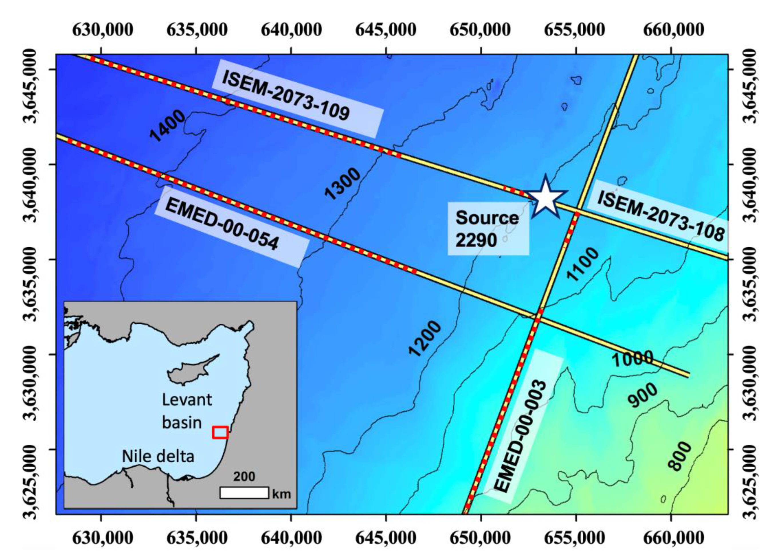
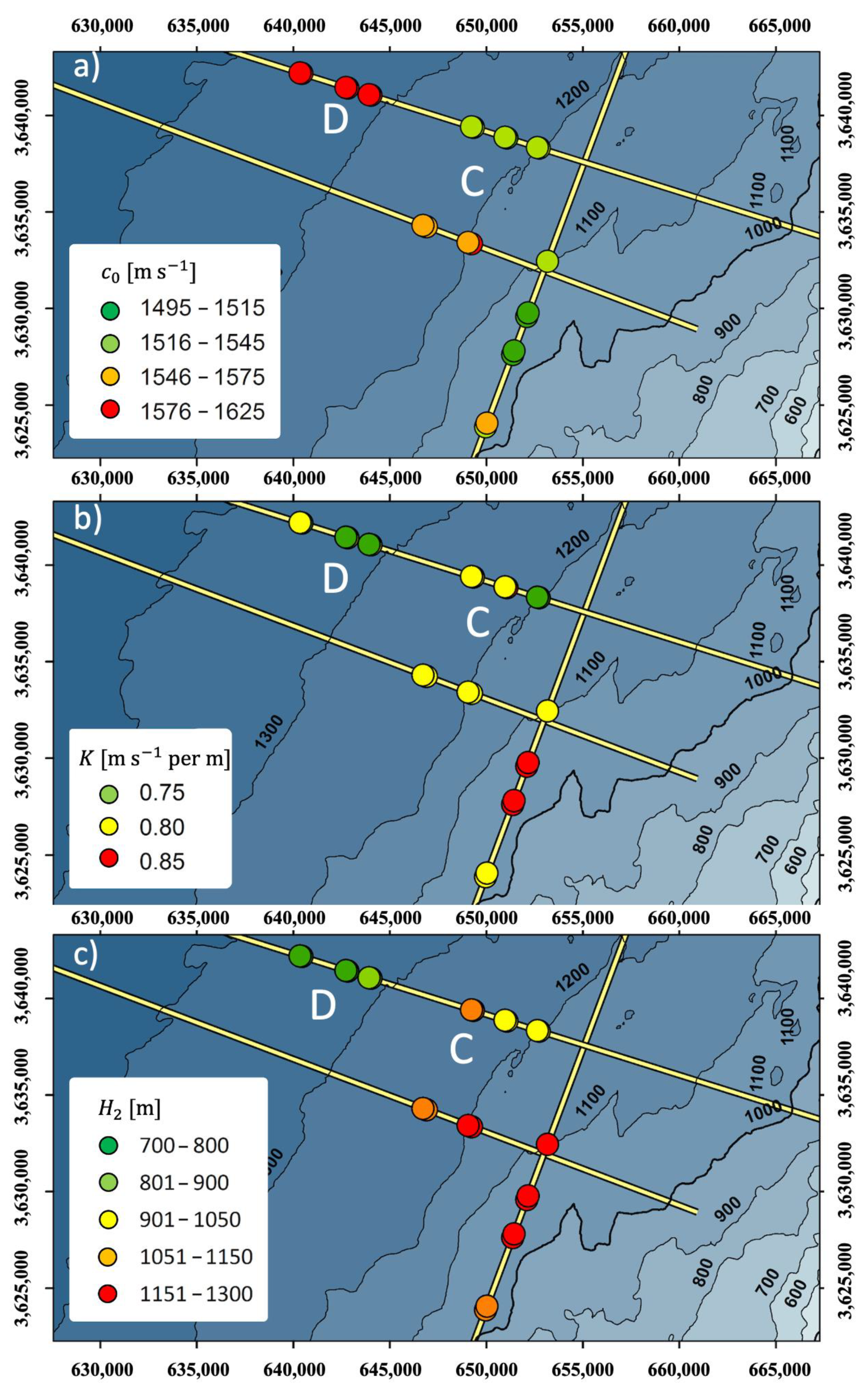
Gradients in the geoacoustic properties of sediments are commonly observed in coring data and in bottom sound-speed inversions [25,37]. They are important to the physics of the scattering process because they control both how the sub-bottom is illuminated [38] and how the scattered field propagates back to the receivers [39]. These gradients in the sub-bottom are usually not smooth and have rather rapid, fluttered fluctuations. However, in seismic work, where the wavelengths of the radiated signals are considerably larger than these fluctuations, the overall representation by analytic functions is of practical value [40].

The variation of the sound speed with sub-bottom depth can be described using various models of differing complexity. For general acoustic problems and common geoacoustic parameters of the seafloor, one can use a homogeneous liquid half-space representation of the bottom. The implementation of a liquid homogeneous half-space bottom model showed its particular applicability for gas-rich lake-floor sediments [3,7]. In this case, the seafloor sound speed was particularly low (~350 m s⁻¹), and the reflection coefficient was found to be exceptionally high ($\left|V\right| ~ 0.8$), due to the significant concentration of gas bubbles. The liquid half-space bottom model has been successfully applied to sound-speed estimations for thin (<1 m thick), gas-saturated layers.

The simplest representation of a multilayered bottom is a piecewise-constant model with a discrete number of horizontal layers, each having a constant sound speed [41]. More complex models, which are associated with the compaction of sediments deposited along ocean margins, assume that the sound speed varies continuously with depth. The classical instantaneous linear velocity model $c_b\left(z\right)=c_0+Kz$ and the classical exponential model $c_b\left(z\right)=c_0\exp \left(\frac{K_{0}z}{c_0}\right)$ [42] are generally accepted and often confirmed by measurements of thin clastic sediment sections [43]. Here $c_0$ is the topmost seafloor sound speed, $K$ is a constant vertical sound speed gradient in the linear model, and $K_a$ is the gradient at the top interface in the exponential model. However, these models increase towards infinity with the increasing thickness of the sub-bottom layer. For large thicknesses, these models no longer represent any physical compaction of the sub-bottom layer [44]. Moreover, in the exponential model, the gradient increases with depth, which contradicts the expected behavior [44,45]. There are other models that represent the bottom velocity structure (e.g., the parabolic model [40] or the linear decrease of slowness [46]), each having its advantages and limitations. Ravve and Koren [44] suggested an asymptotically bounded, exponential-velocity model. Their model better represents the vertical sound-speed variations in compacted sediments, especially in the case of thick layers. For such sediments (e.g., as found in Gulf of Mexico) the gradient is higher in the upper layer and gradually decreases with depth. In practice, seismic velocity is affected by sediment composition, pore shape, pore pressure, pore-fluid saturation and confining pressure, all of which are partly associated with the compaction, and by temperature. These factors may cause local anomalies with respect to the general trend of increased velocity with depth [44].

1.3. The Study Site

This study focuses on the Levant basin seafloor off the base of the southeastern Mediterranean Sea continental margin, offshore Israel (Figure 1). This presently passive, continental margin was formed during the Mesozoic to Neogene eras [47]. Constrained connectivity with the Atlantic Ocean during the Messinian Salinity Crisis resulted in the accumulation of a ~2 km-thick layer of evaporites, primarily salt, within the southeastern Mediterranean basin [48]. The subsequent development of the Nile and its deltaic system, as well as the transportation of clastic sediments along the northeastern shore, resulted in the rapid accumulation of an up to 1.5 km-thick sedimentary wedge that forms the present-day continental margin [49]. In the measurement area, the Messinian evaporites are overlain by a ~1 km-thick compacting section of primarily fine-grained siliciclastic (clay and silt) sediments [50,51]. Water-mass stratification of the southeastern Mediterranean Sea undergoes pronounced seasonal changes, with the development of a warm and salty surface layer through the summer and autumn and the mixing with deeper water in the winter [52] (Figure 2).

The objective of this paper is to present two complementary methodologies, and the corresponding results, for an acoustic characterization of a compacting passive-margin basin setting using standard commercial multichannel seismic data. The estimated parameters are the seafloor compressional sound speed $c_0$, the linear positive sound-speed gradient $K$ below the seafloor, and the thickness of the relevant sub-bottom sedimentary section $H_2$. A basic description of one of these methods was given by Uzhansky et al. [53], and its application is expanded in this paper.

Figure 2. Typical sound-speed profiles for the study area, which were calculated by the equation of Chen and Millero from CTD measurements made near the study are in 2018 [54,55]. These July and November sound-speed profiles were used as the summer- and winter-velocity profiles, respectively, in the top layer of our model.

Figure 2. Typical sound-speed profiles for the study area, which were calculated by the equation of Chen and Millero from CTD measurements made near the study are in 2018 [54,55]. These July and November sound-speed profiles were used as the summer- and winter-velocity profiles, respectively, in the top layer of our model.

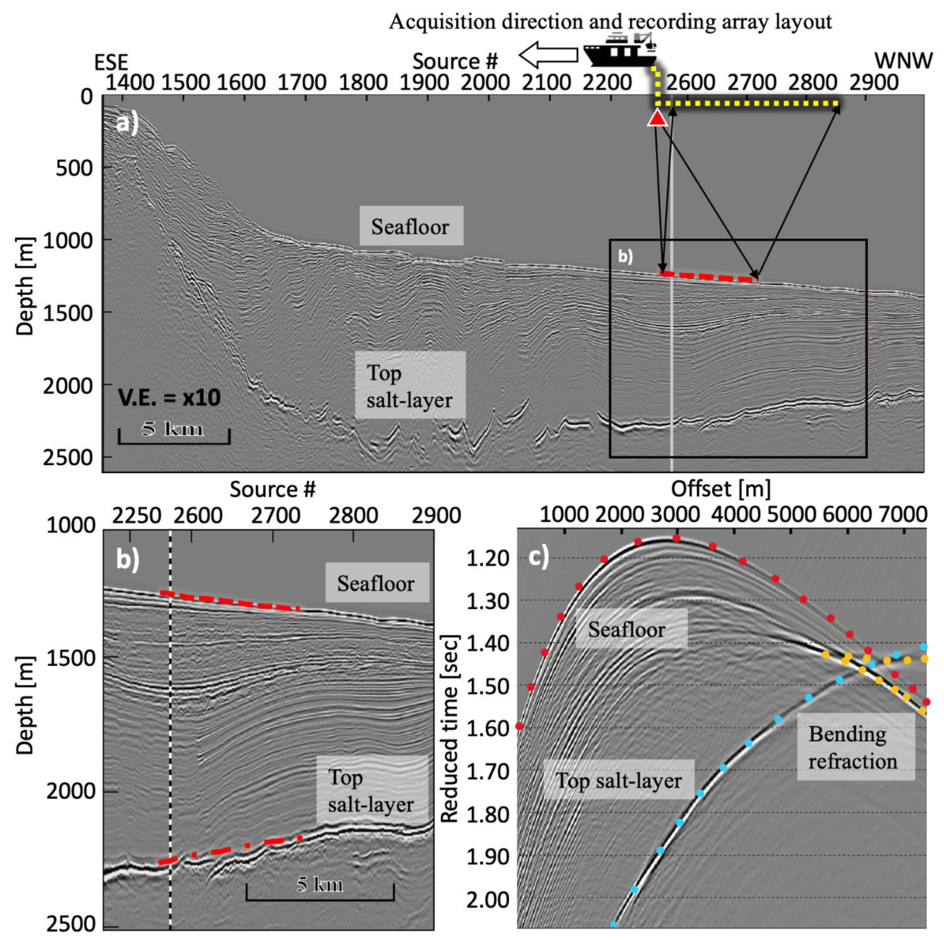
2. The Experimental Data

In this study, we utilized the raw data of two 2D seismic lines of the EMED and ISEM surveys offshore Israel (Figure 1). EMED data were acquired by Spectrum Energy & Information Technology Ltd. of Woking, Surrey, UK, onboard the R/V Geo Baltic on 11 July 2000 (EMED-003) and 2 September 2000 (EMED-054), using a 7200 m-long HLA of 576 hydrophones with 12.5 m spacing that started at an offset (i.e., the distance from the source) of 150 m and was towed at a depth of 10 $\pm$ 1 m. Nine-seconds-long signals were recorded at the sampling interval of 2 ms. The sound was radiated with a Sodera G-Gun consisting of 4 sub-arrays of air guns with a working pressure of 2500 psi and located at a depth of 6 $\pm$ 0.5 m, with a shooting interval of 50 m. ISEM data were acquired by TGS-Nopec Geophysical Company onboard the R/V Northern Access on 11 November 2001, using a 7200 m-long HLA of 576 hydrophones with 12.5 m spacing that started at an offset of 150 m and was towed at a depth of 5 m. Nine-seconds-long signals were recorded at the sampling interval of 2 ms. The sound source consisted of 4 sub-arrays of air guns with a working pressure of 2500 psi and located at a depth of 5 m, with a shooting interval of 25 m. The source signal bandwidth was 20 and 70 Hz with a peak frequency of 35 Hz (Figure 3).

The raw data were loaded into the Emerson Paradigm seismic processing software and geometry was assigned based on the sources’ P190 file coordinates and the HLA layout parameters. Subsequent data processing utilized the Echos modules, including the application of Notch and High-pass filters at the frequencies of 1 and 8–36 Hz, respectively, for noise reduction.

The seismic lines were depth-migrated (Figure S1 supplementary information) in order to constrain the depth model to be used in the subsequent analysis of the raw gathers of records from a single source (source gather). A subsequent velocity analysis focused on areas of simple geology (Figure 1), away from significant seafloor structures that might bias the velocity estimations. Areas of simple geology imply relatively monotonous bottom and sub-bottom geological structure and stratification over the entire seafloor stretch that was insonified by the source-receiver layout (the seafloor ‘footprint’ of this source). This footprint coverage area extended approximately to half the length of the HLA (i.e., L/2 = 3600 m; red dashed line in Figure 4a).

Travel times of the relevant phases were then chosen, assisted by reduced travel-time displays of the data. The reduced travel time is given by:

$$T_{reduced}=T_{arrival}-\frac{x}{c_{reduced}},$$

(1)

where $T_{reduced}$ and $T_{arrival}$ are the reduced and original recording times, respectively, $x$ is the source to the receiver offset, and $c_{reduced}$ is the reduction in sound speed assumed by the user. The travel-time choices were exported into MATLAB for subsequent comparison with simulations.

To consider ray deviation in the water column, characteristic summer and autumn sound speed profiles were calculated from CTD measurements that were obtained near the study area in July and November 2018 [54], using the equation of Chen and Millero [55]. The resulting velocity profile in the water column (Figure 2) was comprised of three layers: (1) a surface layer a with sound speed of 1538 m s⁻¹ in November and 1545 m s⁻¹ in July; (2) a sharp summer thermocline at a depth of ~30 m in July and ~70 m in November, with a minimum at a depth of ~400 m; and (3) a slow but constant increase of sound speed with depth. The sound-speed profile becomes independent on the season after ~180 m of the water depth.

As an example, let us consider the records from sound source #2290 of line ISEM-2073-108 (see the location in Figure 1). Figure 4a,b present a depth-migrated reflection section of line ISEM-2073-108, showing the seafloor in the study area, sloping gently (~0.01°) westwards between water depths of ~1200–1300 m. The top of the Messinian salt layer was imaged at a depth of ~2200 m and a relatively mild structure was observed in the sedimentary overburden below the seafloor footprint of source #2290. This image was used to constrain the travel-time modeling of travel times recorded from this source. Figure 4c depicts a reduced time vs offset display of the source #2290 records, overlaid with the picked phases, including the seafloor reflection, top-salt reflection, and bending rays’ refraction.

2.1. Methodology for Seafloor Sound Speed Estimation Based on Travel Times Matching

The critical distance (the minimum distance at which the head wave can be registered on the HLA records) increases with the bottom depth, and with a decrease in the acoustic impedance contrast at the seafloor [36]. For a constant sound speed in the water layer, the minimum distance at which the seafloor interface head wave can be registered with a Horizontal Line Array (e.g., the black solid line in Figure 5) is

$$R_c=2H_1\tan \left({\theta }_c\right),$$

(2)

where $H_1$ is the bottom depth, ${\theta }_c=\mathrm{asin}\frac{c_w}{c_0}$ is the critical angle of incidence, $c_w$ is the sound speed in the water near the seafloor, and $c_0$ is the sound speed at the seafloor. An additional offset coverage is needed to properly identify the seafloor interface head wave refracted arrival in the HLA’s records (e.g., as depicted by a dashed line in Figure 5). For high-sound-speed seafloors, such as coarse sand, gravel, and basalt, $R_c$ is significantly smaller than the length, $L$, of the HLAs, which are commonly used for 2D marine seismic data acquisition and are 7200 m in our case. However, for the common abyssal seabed with a relatively low sound speed (e.g., with a predominantly silt to clay composition with $c_0$~1500–1600 m s⁻¹) [10] $R_c$ becomes bigger than $L$, and an alternative approach is required for the estimation of the seafloor sound speed based on data recorded by such HLAs. In the following section, we exploit acoustic rays that bend and reach the critical angle below the seafloor, where the sound speed increases with the depth.

The essence of the methodology introduced in this study is a geoacoustic inversion, which is based on the recursive matching of experimentally recorded and simulated acoustic–seismic arrival times. Reduced-time (Equation (1)) displays were applied to facilitate the comparison of experimental and simulated arrival times. For horizontal interfaces, if the assumed sound speed matches the refractor sound speed, then the refraction will display as a horizontal line on the reduced time vs. offset plot. Arrivals with an assumed sound speed lower than the reduction velocity will have a positive slope, whereas those with a sound speed greater than the reduction velocity will have a negative slope. Three alternative methodologies for calculating the arrival times of head-wave refractions correspond to three cases of water and bottom stratification:

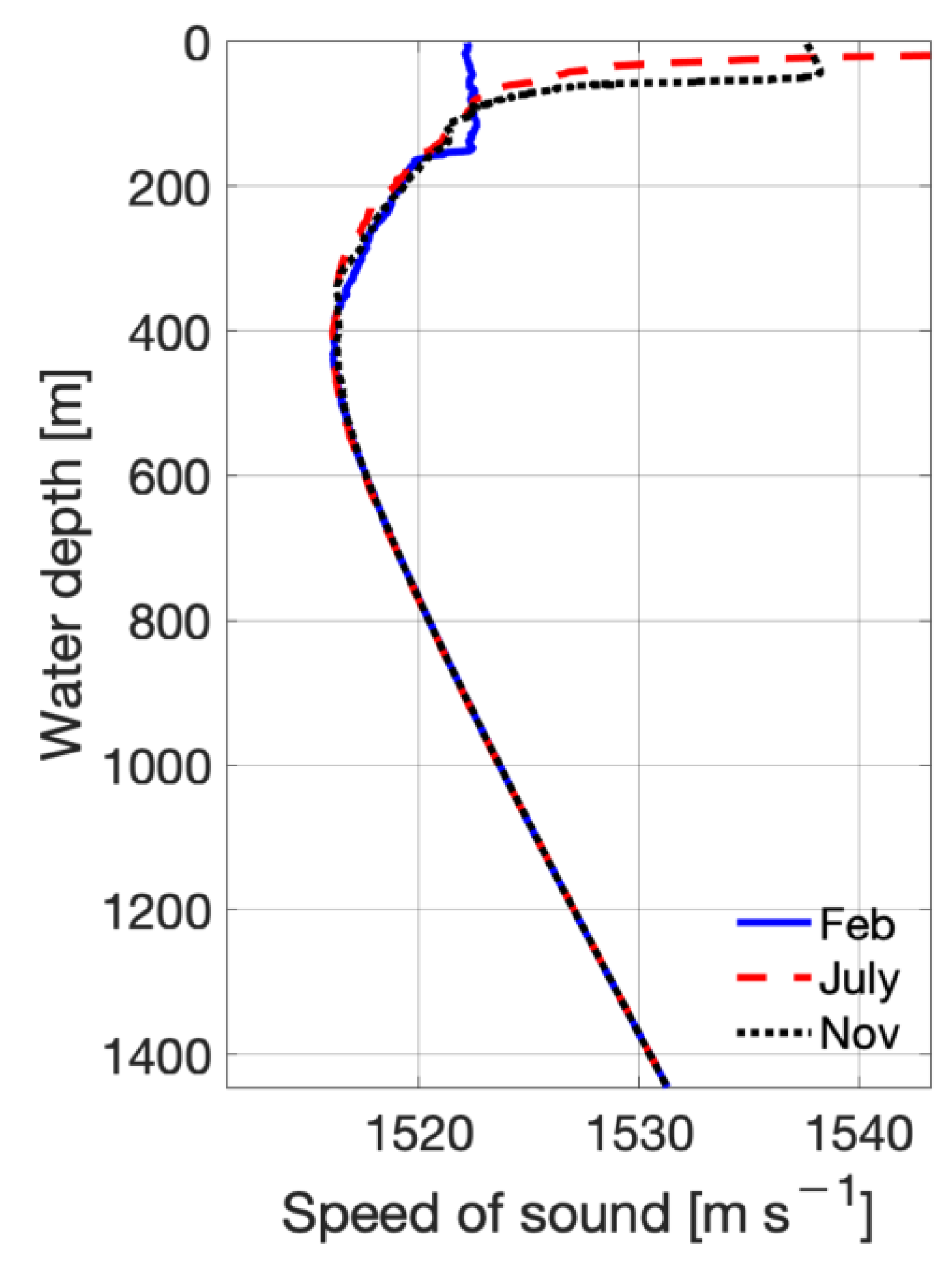
2.2. Constant Sound Speed in the Water Layer

For homogeneous horizontal layers, the range $x_1$ and time $t_1$ for a ray propagating through this layer and back to the surface can be described as a function of the ray parameter $p$ using the relationships:

$$\begin{array}{c}{x}_1=\frac{2H_1}{\sqrt{1-{\left(p{c}_w\right)}^2}}\\ t_1=\frac{2H_1}{c_w}\frac{1}{\sqrt{1-{\left(p{c}_w\right)}^2}}\end{array}\}, 0\le p<\frac{1}{c_w},$$

(3)

where $H_1$ is the thickness of the water layer, ${\alpha }_w$ is the angle of incidence, $c_w$ is the sound speed in the water, and the slowness $p=\frac{\sin {\alpha }_w}{c_w}$.

2.3. Constant Sound Speed in the Water and a Constant Velocity Gradient in the Sub-Bottom Layer

For a sub-bottom layer with a vertical velocity gradient, the range $x_2$ and time $t_2$ of diving rays refracting from this layer can be described according to [35,56] as:

$$\begin{array}{c}{x}_2=\frac{2}{Kp}\sqrt{1-p^2{c}_0^2}\\ t_2=\frac{2}{K}\left[\log \frac{1+\sqrt{1-{\left(p{c}_0\right)}^2}}{c_{0}p}\right]\end{array}\}, 0\le p<\frac{1}{c_0},$$

(4)

where $c_0$ is the sound speed at the seafloor and $K$ is the gradient in the sub-bottom layer.

When the source and receivers are located in the homogeneous water layer, the travel-time curve consists of two parts: the reflection travel-time curve is given by Equation (3) and the travel-time curve of the refraction of diving rays is given by the summation of Equations (3) and (4). The reflection travel-time curve is a hyperbola. The refraction forms a bow-tie curve with up to two cusps (i.e., turning points), depending on the parameters of $c_w$,$c_0$, $H_1$, and $K$.

2.4. Stratified Water and a Constant Velocity Gradient in the Sub-Bottom Layer

For the more realistic case, when the acoustic velocities of both the water and bottom media vary with depth (Figure 6), no analytical expression is applicable to calculate the travel-time curves. These calculations require numerical modeling, e.g., of ray travel times. In our case, the BELLHOP [57] ray-tracing program, which is freely available at the Ocean Acoustic Library as a part of the Acoustic Toolbox, was used.

Calculations were done in two steps. First, the travel times of the direct arrival and the seafloor reflection were calculated. The model consisted of a water layer of thickness $H_1$ with a seasonally changing oceanographic stratification, bottoming at a flat horizontal seafloor. Afterwards, the arrival times of the bending refraction and the sub-bottom reflection from the top of the salt layer, at the base of the sub-bottom sequence, were calculated. In BELLHOP, after reflection at the boundary, the beam is only reflected and does not penetrate further into the second medium. Thus, in order to calculate the bending refraction and the sub-bottom reflection, the seafloor must be removed from the model. For this, the water layer of thickness $H_1$ and the bottom layer of thickness $H_2$ were combined into one layer of thickness $H_1+H_2$, keeping the variability of the sound speed. Ray travel distances were calculated from ray coordinates that were obtained using BELLHOP. After calculating the rays’ travel paths and distances, the rays’ travel times were calculated by dividing the travel distance by the sound speed at every given depth. Note that at this step we are interested only in ray travel times and not in sound pressure. That is why neither the densities nor the attenuation coefficients of the media are needed.

Comparing the modeling results that were carried out with a constant-velocity water layer with the results of using the summer- and winter-velocity profiles (Figure 2) reveals some differences: (1) Changes in the offsets at which specific rays bend and reach the seafloor, particularly at low grazing angles. For example, a ray with a grazing angle of 29° bended and reached the surface at offsets of 7250, 7150 and 6900 m when modeled with a constant velocity, winter and summer water profiles, respectively. In contrast, a ray with a grazing angle of 16° bended at offsets of 7300, 6200 and 5100 m, respectively. (2) Differences in arrival travel times. Primarily, differences of up to 0.082 s were observed in the arrival times of the direct wave at a specific offset between the constant-velocity and summer-velocity profiles. Within the range of our modeled travel times (to 7200 m) the differences in the travel times of reflected and bending rays were small. However, more substantial time differences may be encountered at larger offsets. (3) The first angle at which rays start bending beneath the seafloor is reduced in the realistic-velocity case, with respect to the constant-velocity case.

2.5. The Geoacoustic Inversion Procedure

The ray travel-time branches, which were extracted from the experimental source gather (Figure 5), were numerically compared to the modeled ray travel-time branches. The comparison was made both for the vertical (travel time) and horizontal (offset) axes of the travel-time branches. In practice, the travel time branches were defined by five points: two points for the top-salt reflection (SB1 and SB2), and three points at the edges of the two travel-time branches of the bending rays (BR1, BR2, BR3) (red squares, Figure 7b). The top-salt reflection points SB1 and SB2 were chosen at the constant offsets of 1000 and 5500 m, respectively. The bending refraction points were chosen as follows: BR1 was located at the cross-point of the bending refraction and the seafloor reflection, BR2 was a turning point (cusp) of the refraction travel-time curve, and BR3 was located at the end of the HLA at the distance of 7350 m from the source. This procedure was then repeated for each unique triplet of $c_0$, $K$, and $H_2$ across ranges of each of these parameters with step sizes of 5 m s⁻¹, 0.05 s⁻¹, and 50 m, respectively. In each case, the deviation of the modeled travel-time marker points from the modeled ones was evaluated by computing the error function

$$E\left(c_0,K,H_2\right)=\frac{1}{N}{\displaystyle \sum }_{n=1}^N\sqrt{{\left(X_{exp\_n}-X_{\mathrm{mod}\_n}\right)}^2+{\left(T_{\exp \_n}-T_{\mathrm{mod}\_n}\right)}^2},$$

(5)

where $N$ is the number of analyzed experimental points,$X_{\exp \_n}$,$X_{\mathrm{mod}\_n}$ are normalized experimental and modeled offsets, and $T_{\exp \_n}$, $T_{\mathrm{mod}\_n}$ are normalized experimental and modeled two-way reduced arrival time, of each of the marker points. In order to balance the impact of the horizontal and vertical components of the arrivals, both experimental and modeled arrival times and the offsets are normalized such that their maximum is 1. In our case, the offsets were normalized by 7350 m (the maximum offset of the HLA used), and the reduced arrival times were normalized by 4.2 s (the maximum offset of 7350 m divided by the roughly assumed average sound speed in the sub-seafloor medium of 1750 m s⁻¹; Figure 7b). Once the computation was complete, the normalized weight function was computed as

$$F\left(c_0,K,H_2\right)=\frac{\left| E-\max \left(E\right)\right|}{\max \left(\left|E-\max \left(E\right)\right|\right)},$$

(6)

where $E=E\left(c_0,K,H_2\right)$ (Figure 8a–c). The best fit between the normalized experimental and the simulated ray travel times and distances corresponds to the maximum of the weight function, constraining the combined estimate of the geoacoustic parameters $c_0$-$K$-$H_2$.

Figure 7a represents an example of the normalized weight function $F_{norm}\left(K,c_0, H_2{}_{best}\right)$, where $H_2{}_{best}$ = 1000 m was chosen from the highest $F\left(c_0,K,H_2\right)$, i.e., the best fit, for source #2290. The combination of $c_0$ and $K,$ for which the arrival of the bending refraction exceeded 7,200 m, was omitted from the estimations of $F$ (white in Figure 7a). Source #2290 $F_{norm}\left(K,c_0\right)$ had a maximum at $c_0$ = 1535 m s⁻¹ and $K$ = 0.75 s⁻¹, from which it was gradually decreasing in all directions.

Figure 7b depicts a set of arrival times that were simulated for three combinations of $c_0$, $K$, and $H_2$ and overlaid with the experimentally chosen arrival times (white circles) from source gather #2290. The model strongly deviates from the experiment when $c_0$ and $K$ are either too low (blue dash-dot curve) or too high (green dotted curve).

Figure 8a–c demonstrate the sensitivity of the geoacoustic inversion by separately showing the sensitivity of the normalized probability functions to each of the parameters, $F\left(c_0,K_{best},H_2{}_{best}\right)$, $F\left(c_{best},K,H_2{}_{best}\right)$, and $F\left(c_{best}, K_{best}, H_2\right)$. Here $c_{best}$, $K_{best}$, and $H_{best}$ are the best fit estimated between the experiment and the models, i.e., the set of matching parameters for which $F\left(c_0,K,H_2\right)$ is the highest. The margin of error for the estimation of $c_0$, $K$, and $H_2$ is estimated to correspond to the width of the respective weight function at the level above 0.95 of the maximal value (dashed line in Figure 8a–c).

Figure 8d–i represent a set of modeled reduced times, overlaid with experimentally chosen reduced travel times, and their zoomed portions, respectively. Each row emphasizes the influence of a specific parameter, $c_0$, $K$ or $H_2$, on the modeled arrival times. In Figure 8d,g, the arrival times are modeled for the constant parameters $K$ = 0.75 s⁻¹, $H_2$ = 1000, and $c_0$ = 1430, 1535, 1600 m s⁻¹. The best match between the model and the experiment is achieved for $c_0$ = 1535 m s⁻¹. If the sound speed is relatively low (i.e., $c_0$ = 1430 m s⁻¹), both the sub-bottom reflection and bending refraction travel-time branches deviate significantly downward and exhibit greater offsets from the experimental points (blue dash-dot curves). In contrast, if the sound speed is high, i.e., $c_0$ = 1600 m s⁻¹, both the sub-bottom reflection and bending refraction travel-time branches deviate upward and exhibit lesser offsets from the experimental points (green dotted curves).

Figure 8e,h represent a situation where $c_0$ = 1535 m s⁻¹ and $H_2$ = 1000 m, and $K$ is varying from 0.6 to 1 s⁻¹. The best match is achieved when $K$ = 0.75 s⁻¹. In a manner similar to the previous situation, when $K$ is too high or too low, both the sub-bottom reflection and bending refraction travel-time branches significantly deviate (by ~0.1 s) from the experimental data. Figure 8f,i represent a case in which $c_0$ = 1535 m s⁻¹ and $K$ = 0.75 m s⁻¹, but $H_2$ varies from 900 to 1200 m. In contrast to the two previous cases, there was no difference in the arrival times and position of the modeled bending refraction travel-time branch. The only difference was the increasing length of its upper part. This is demonstrated in Figure 8i at the offset of about 6500–7000 m, where only the refraction modeled for $H_2$ = 1200 m crossed the seafloor reflection. However, the modeled arrivals of the sub-bottom reflection at the offset of 1000 m deviated by up to 0.6 s and reduced to ~0.02 s at high offsets (~6000 m). This resulted in one prominent peak of the weight function $F_{norm}\left(c_{best},K_{best},H_2\right)$, as depicted in Figure 8c.

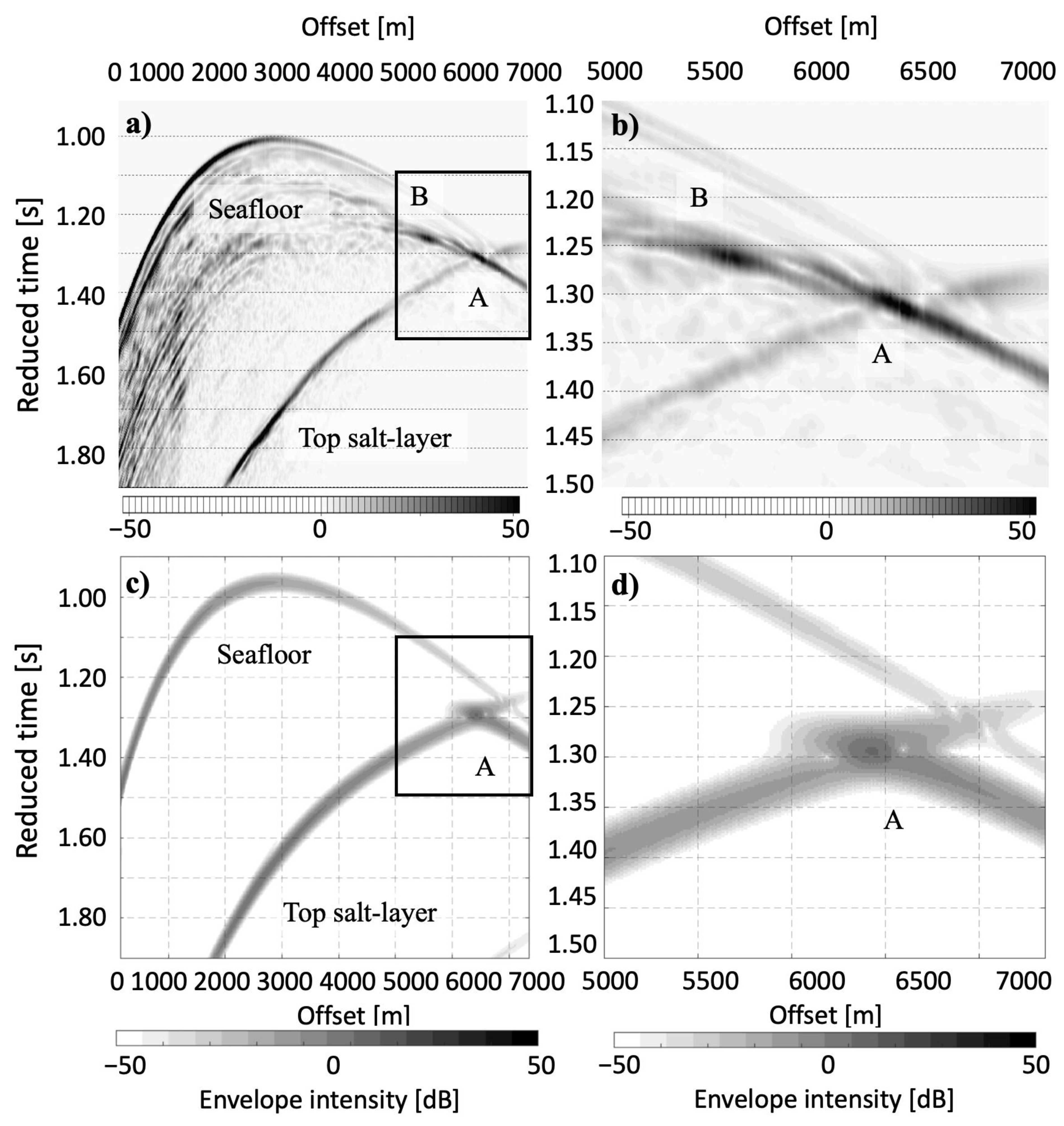
2.6. Validating the Sound-Speed Estimations through Caustic Amplitude Modeling

A second way to estimate $K$ is by using caustic amplitude modeling. As shown in the previous section, the acoustic–seismic rays may bend significantly while propagating through the water and sub-bottom layers. Due to bending, a range of rays may at some point focus and intersect (Figure 6), causing a significant increase in sound intensity (i.e., forming a caustic). The formation and shape of such a caustic is sensitive to the velocity gradient. Thus, identifying such caustics in the experimental data and matching them with simulation results can constrain the value of $K$. For this study, we carried out preliminary caustic amplitude modeling for select sets of $c_0$, $K$, and $H_2$, in order to validate the estimations that were obtained from our travel-time-based geoacoustic inversion. Section 4.5 in [36] presents an analytical formula for $K$, which makes use of the caustic’s position.

In the following model, the sound speed in the water is constant and equals the topmost sound speed at the seafloor. In the sub-bottom layer, the sound speed is linearly increasing with depth as $c_b=c_0+Kz$. For such a model, the linear positive sound-speed gradient can be expressed as

$$K=8c_0\frac{2H_1-z_s-z_c}{r^2},$$

(7)

where $z_s$ and $z_c$ are the depths of the sound source and caustic, respectively, $r$ is the range between them, and $H_1$ is the depth of the seafloor. For the more complex case of a vertically varying water column and a specific sound speed at the seafloor, the position and intensity of such a caustic can be numerically calculated via the modeling of a broadband sound-field propagation, for instance, by using a parabolic equation approach. The parabolic equation is a powerful approach for solving inseparable wave propagation problems, for which: (1) the properties of the medium vary gradually in range (in the horizontal directions), but may have strong vertical variations; and (2) energy that propagates outward in range dominates energy that scatters back toward the source [58,59]. In comparison to the conventional approaches of Ray Theory and Normal Modes, the Parabolic Equation method combines computation efficiency and accuracy when the depth of the model (in the order of kilometers in our case) is much bigger than the wavelength and many radiation angles are considered. Parabolic Equation approaches do not consider very small angles of incidence, which can be neglected for high ranges (order of kilometers) due to high attenuation. Thus, here we use the Parabolic Equation approach to model a synthetic source gather for its consequent comparison with the experimental one (Figure 4c). To approximate the experimental wavelet of Figure 3 we used a Ricker wavelet with a similar spectral content (Figure 9; [60]).

For a more robust estimation of $c_0$, $K$, and $H_2$, one can perform a full geoacoustic inversion of the intensity and arrival time of the caustic, using a weight function like the one described in the previous section (Equations (5) and (6)).

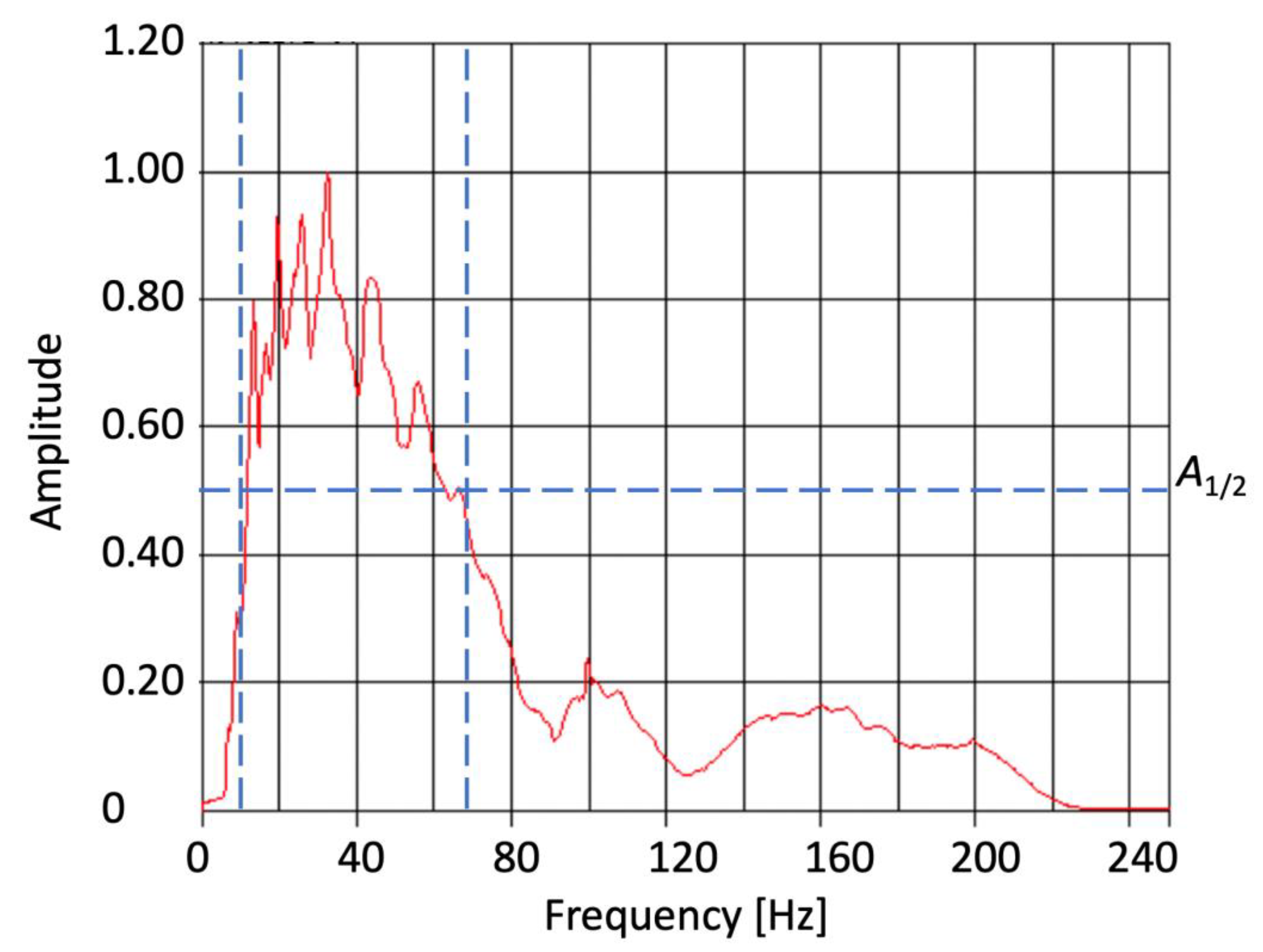
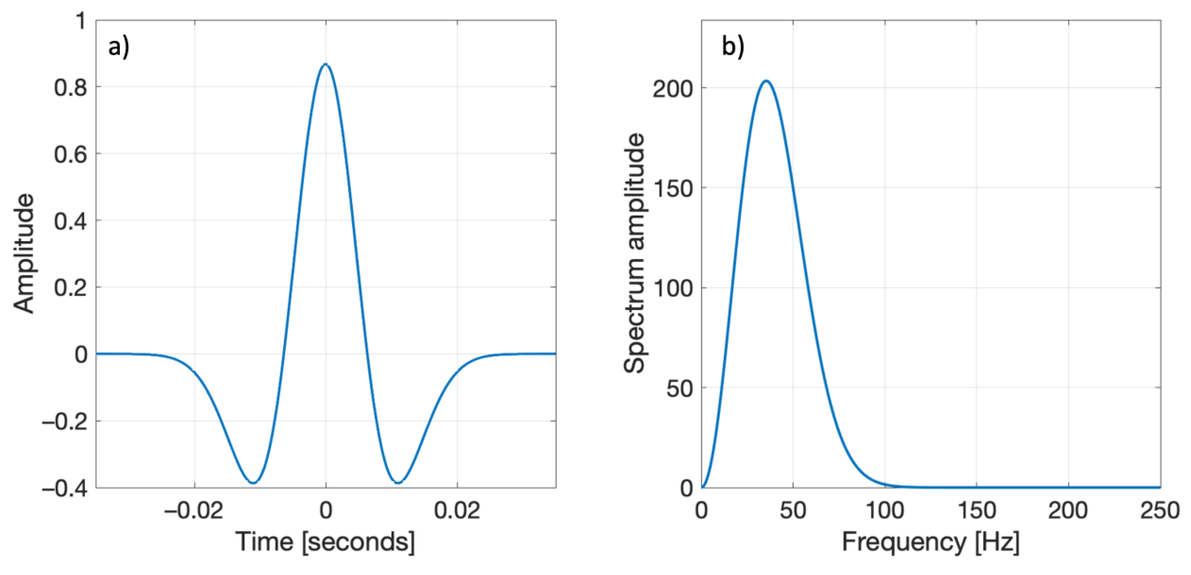
2.7. The Ricker Wavelet

The Ricker wavelet is a theoretical waveform obtained by solving the Stokes differential equation [60,61]. This type of wavelet is representative of seismic waves propagating through viscoelastic homogeneous media because it matches the effects of Newtonian viscosity. Mathematically, the Ricker wavelet is the second order derivative of a Gaussian function. Being zero-phase, it is symmetric in the time domain. In reality, seismic signals are usually minimum-phase, and are therefore similar to the first or one-and-a-half derivatives of a Gaussian function [61,62]. Notwithstanding, various derivatives of a Gaussian function have similar amplitude spectra that are different from a Gaussian distribution. The Ricker wavelet is commonly used in seismic analysis, for instance, in wave field simulations or reflectivity inversions [63].

The Ricker wavelet is defined in the time domain as

$$r\left(\tau \right)=\left(1-\frac{1}{2}{\omega }_p^2{\tau }^2\right)\exp \left(-\frac{1}{4}{\omega }_p^2{\tau }^2\right),$$

(8)

where $\tau$ is time (in seconds) and ${\omega }_p$ is the most energetic frequency (in radians per second). It is symmetric in the time domain and has a zero mean, as ${\int }_{-\infty }^{\infty }r\left(\tau \right)d\tau =0$. The Fourier transform of the Ricker wavelet may be expressed as

$$R\left(\omega \right)=\frac{2{\omega }^2}{\sqrt{\pi } {\omega }_p^3}\exp \left(-\frac{{\omega }^2}{{\omega }_p^2}\right),$$

(9)

where $\omega =2\pi f$ is the angular frequency and $f$ is the frequency in Hz.

For our modeling of a synthetic source gather we selected a Ricker wavelet (Figure 9) with similar spectral characteristics as the experimental data (Figure 3). Both have a frequency content of 20 to 70 Hz and a peak frequency at 35 Hz.

2.8. Modeling of a Synthetic Source Gather

A synthetic source gather represents a modeled field that could be registered by an HLA of hydrophones recording arrivals from a single instant source. It represents the amplitude of the recorded sound as a function of its arrival time (two-way travel time) and offset.

To model such a source gather, we calculated multiple single-frequency sound fields at the frequency band of the air gun (i.e., wide band) and transformed their sum from the frequency domain into the time domain using the inverse fast Fourier transform. The sound fields were modeled with the range-dependent acoustic modeling software RAM [64], which is based on the split-step Padé solutions of the parabolic equation [65]. The sound pressure was calculated with the aforementioned parabolic equation solution as follows:

$$p\left(r+\mathsf{\Delta }r,z\right)=\exp \left(i{k}_0\mathsf{\Delta }r\sqrt{1+X}\right)p\left(r,z\right),$$

(10)

where $X=k_0^{-2}\left(\rho \frac{\partial }{\partial z}\frac{1}{\rho }\frac{\partial }{\partial z}+k^2-k_0^2\right),$

$k=\left(1+i\eta \alpha \right)\frac{\omega }{c},$

$\eta ={\left(40\pi {\log }_{10}e\right)}^{-1},$

$\rho$ is the density, $\alpha$ is the attenuation in dB per wavelength,

$\omega$ is the cyclic frequency, $c$ is the typical phase speed in the media,

$k_0=\frac{\omega }{c}$ is the wavenumber.

As above, we show here the modeling results for the case of source gather #2290 in profile ISEM-2073-108. Our geoacoustic model consisted of three layers: (1) a layer of thickness $H_1$ and a sound speed profile $c_w$ that vary with seasonality, (2) a sub-seafloor layer of thickness $H_2$ and the sound speed at the seafloor $c_0$, which increased with depth due to a positive sound-speed gradient $K$, and (3) a salt layer of infinite thickness with a sound speed of 4000 m s⁻¹. The density of the second layer at the seafloor was 1250 kg m⁻³, according to measurements we made on a sediment core that was obtained in the study area. In our model we assumed that the density in the second layer was increasing linearly according to the equations of Akal (1972), in correlation with the sound speed, and reached 2500 kg m⁻³ at the bottom of the second layer (i.e., the depth of the top-salt interface).

Figure 10 compares the experimental and modeled source gathers. The synthetic gather was modeled for $c_0$ = 1535 m s⁻¹ and $K$ = 0.75 s⁻¹, which were found by the geoacoustic travel-time inversion that best fit the experimental data (Figure 7 and Figure 8). Arrival A is a possible caustic that was found in the experimental data and is matched by our model. Arrival A follows a significant intensity increase (by ~30 dB) at the range of ~6200 m, which is associated with the arrival of the caustic. B is another high-intensity arrival, which can possibly be another caustic from a sub-bottom layer, or another sort of reflection from sub-bottom layering.

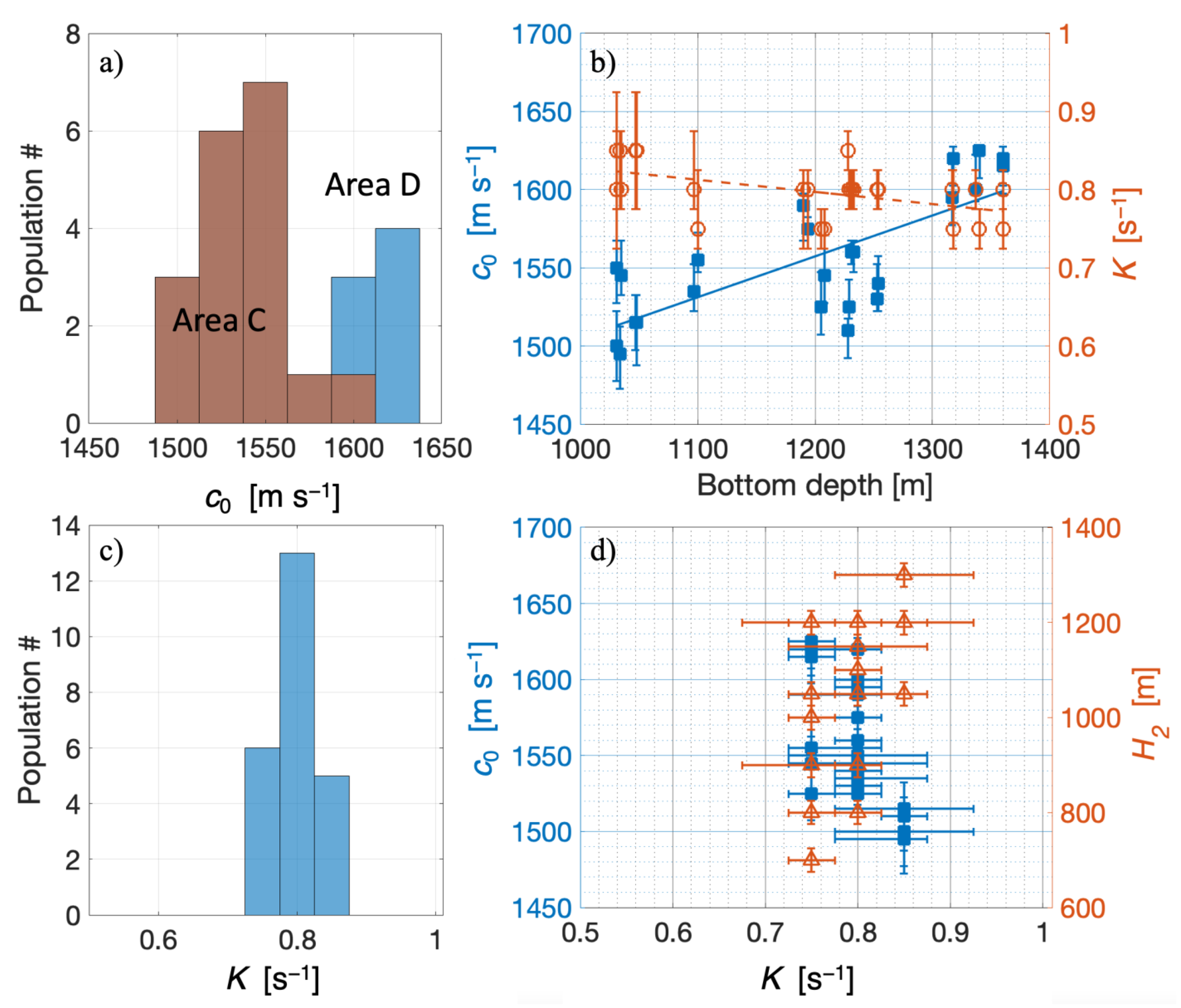
3. Inversion Results

In total, the bottom parameters, including $c_0$, $K$, and $H_2$, were examined in 24 locations, distributed in the regions of our study area that had relatively simple geology (Figure 1; red dashed lines). These were composed of 12 adjacently located pairs in order to verify the consistency of the results. The results of our geoacoustic inversion are summarized in

Table 1. The parameters estimated in the study area. The range of the geoacoustic parameters $(c_0,K)$ in which the normalized $F\left(c_0,K,H_2\right)$ is >0.95 of its maximum level, F_0.95, represents the estimation error. FFID is a Field File Identification Number, i.e., the source gather number.

Line Name	FFID #	x [m]	y [m]	${\mathit{H}}_1$ [m]	${\mathit{c}}_0$ [m s−1]	${\mathit{c}}_0 \mathbf{for} {\mathit{F}}_{0.95}$ [m s−1]	$\mathit{K}$ [s−1]	$\mathit{K} \mathbf{for} {\mathit{F}}_{0.95}$ [s−1]	${\mathit{H}}_2$ [m]
EMED-00-003	2670	649,974	3,623,866	1035	1545	1535–1565	0.8	0.8–0.85	1150
	2674	650,043	3,624,054	1031	1550	1530–1565	0.8	0.75–0.85	1150
	2750	651,373	3,627,613	1031	1500	1480–1520	0.85	0.8–0.9	1200
	2754	651,441	3,627,801	1034	1495	1475–1510	0.85	0.8–0.85	1200
	2792	652,106	3,629,580	1047	1515	1500–1530	0.85	0.8–0.9	1300
	2796	652,173	3,629,769	1048	1515	1490–1530	0.85	0.8–0.9	1300
	2853	653,171	3,632,438	1097	1535	1525–1550	0.8	0.8–0.85	1200
	2857	653,239	3,266,326	1100	1555	1550–1570	0.75	0.75–0.8	1200
EMED-00-054	351	649,245	3,633,347	1190	1590	1570–1595	0.8	0.75–0.8	1200
	355	649,059	3,633,419	1194	1575	1565–1580	0.8	0.75–0.8	1200
	401	646,906	3,634,230	1231	1560	1555–1565	0.8	0.8–0.8	1100
	405	646,720	3,634,302	1233	1560	1550–1565	0.8	0.8–0.8	1100
ISEM-2073-108	2290	652,744	3,638,304	1205	1525	1510–1545	0.75	0.75–0.75	1000
	2294	652,650	3,638,335	1208	1545	1530–1560	0.75	0.75–0.75	1050
	2360	651,076	3,638,831	1228	1510	1495–1515	0.85	0.85–0.85	1050
	2364	650,980	3,638,859	1229	1525	1520–1540	0.8	0.8–0.8	1050
	2433	649,333	3,639,371	1253	1530	1525–1550	0.8	0.8–0.8	1100
	2437	649,238	3,639,400	1254	1540	1525–1555	0.8	0.8–0.8	1100
ISEM-2073-109	2650	644,018	3,641,039	1317	1595	1580–1620	0.8	0.8–0.8	900
	2654	643,922	3,641,067	1318	1620	1605–1625	0.75	0.75–0.8	900
	2700	642,825	3,641,410	1337	1600	1595–1620	0.8	0.8–0.8	800
	2704	642,730	3,641,441	1340	1625	1610–1625	0.75	0.75–0.75	800
	2800	640,444	3,642,168	1360	1615	1600–1625	0.75	0.75–0.75	700
	2804	640,348	3,642,197	1360	1620	1605–1625	0.8	0.8–0.8	800

, and the distributions of these parameters is investigated in Figure 11 and Figure 12.

The constrained seafloor-velocity $c_0$ values show a bi-modal distribution (Figure 11a,b) that is associated with two main parts of the study area (C and D in Figure 12). These two areas correspond to bottom depths of 1030–1250 m and 1320–1360 m, respectively. In area C, sound speed was distributed between 1500 and 1600 m s⁻¹, with an average of 1537 $\pm$ 13 m s⁻¹. In area D, sound speed was markedly higher and was distributed between 1595 and 1625 m s⁻¹, with an average of 1613 $\pm$ 12 m s⁻¹ (Figure 11a,b)_. The average sound speed over the whole studied area was 1556 $\pm$13 m s⁻¹. Thus, $c_0$ seems to increase with the bottom depth $H_1$ (Figure 12a).

$K$ was normally distributed over the whole study area between 0.75 and 0.85 m s⁻¹ with an average of 0.80 $\pm$ 0.035 s⁻¹ (Figure 11c) and seems to slightly decrease with bottom depth $H_1$ (Figure 11b and Figure 12b).

The thickness of the sub-bottom layer $H_2$ varied from 700 to 1300 m and decreased with bottom depth, which agrees with the depth-migrated seismic section crossing the study area (Figure 4a).

Neither the seafloor velocity $c_0$ nor the depth of the salt layer $H_2$ seemed to correlate to the velocity gradient $K$ (Figure 11c,d). This reinforces our assumption that there is no inter-dependence on the geoacoustic estimations. The spatial distribution of the estimated values (Figure 12) demonstrates the consistency of the parameters and their variations between the different seismic lines.

4. Discussion

This paper is focused on the cost-effective, measurement-based geoacoustic characterization of the seafloor at a relatively large water depth (1000–1350 m), in a compacting passive-margin-basin setting, which is globally common. The characterization was achieved by applying a geoacoustic inversion procedure to commonly acquired commercial 2D multichannel seismic-reflection-profiling data. A practical methodology is presented here for using such data for the estimation of the compressional sound speed in the seafloor and compacting sub-bottom, which is characterized by a significant sound-speed gradient.

4.1. Advantages and Constraints of Our Estimation Methodology

The geoacoustic characterization of the seafloor at large water depths requires the use of several kilometer-scale acoustic arrays, the implementation of which is difficult and costly. Our utilization of commercial 2D multichannel seismic-profiling data offset the need for extensive designated acoustic measurement layouts, utilizing instead the standard seismic streamer as an HLA. As a rule, conventional marine seismic acquisition utilizes air-gun arrays as energy sources [66,67]. These are normally tuned to provide sharp- and high-power, downward-propagating signals, which provide deep penetration into the seafloor and high signal-to-noise ratios of reflected and refracted phases over ranges of many kilometers. However, with their primary frequency content being in the tens of Hz, seismic-profiling data provide unusually low-frequency measurements with respect to common acoustic applications. Thus, our results are low-frequency estimates of the geoacoustic parameters. Indeed, the actual velocity at the seafloor, where water content in the sediments is high, is not expected to depend on the frequency, suggesting the general validity of our estimated values. In turn, the estimated gradient may represent the average trend of multiple velocity layers.

Our geoacoustic estimation methodology is a practical extension of Stephen’s [35] simplistic analytic formulation for interpreting the sound-speed structure of the upper oceanic crust from data on the wide-angle reflections and the travel times of the head waves of bending rays from sonobuoy and ocean-bottom reflection experiments. Both approaches are based on the theoretical formulation of Nettleton [56]. However, our modeling was based on the precise numerical calculations of ray travel times, which were carried out here with BELLHOP [57] and MATLAB software. Moreover, we presented a conceptual integration of recursive modeling with an organized geoacoustic inversion, which provided a simultaneous estimation of both the seafloor velocity $c_0$ and the sub-bottom velocity gradient $K$. Importantly, this estimation correctly accounted for a realistic velocity profile in the water column, which may have a significant impact on the calculations at the higher angles of incidence, thereby improving the accuracy of the geoacoustic estimations. The estimations were further constrained by the modeling of a prominent reflection from the base of the sub-bottom constant-velocity-gradient layer, which is the top-salt reflection, constraining its sub-seafloor depth $H_2$.

Here we applied our methodology to a relatively simple case, considering only the vertical variation of the velocity structure and a constant-velocity gradient beneath the seafloor. Such an approximation is generally accepted to represent sediment compaction and is often confirmed by measurements of clay or silt clastic sediments [44]. In reality, the velocity gradient is not necessarily linear. However, building on a standard set of modeling tools, our procedure is directly expandable to allow for a more complex velocity structure. Such structures may be incorporated into the other sub-bottom trends, such as (1) exponential [42], (2) parabolic [40], (3) Faust law [68], (4) using slowness [46], (5) quadratic law, (6) instantaneous velocity [69], or (7) exponential asymptotically bounded velocity model [44]. Moreover, our procedure allows for the relatively simple integration of the lateral variability of the seafloor and the sub-seafloor structure.

The results of the travel-time-based estimation were validated here through caustic amplitude modeling. An analytical expression (Equation (7)) for estimating velocity gradients based on the position of caustics was suggested, for instance, by [36,70], and can be used for rough preliminary estimations. However, our work suggests a conceptual procedure for the combined geoacoustic inversion of both the position and intensity of the caustics, matching the experimental data with wide-band synthetic-source-gather modeling.

The normalized weight function, which was produced by our geoacoustic inversion procedure, had a well-defined single maximum, implying that the estimates obtained are unique. This implication is subject to the assumptions embedded in our modeling, namely the presence of a generally increasing velocity gradient below the seafloor that formed a single caustic in the recorded data. Moreover, the investigation of the normalized weight function allowed us to assess the uncertainties associated with our estimates. Our suggested measure of uncertainty, the 95% level of the normalized weight function, implied accuracies of ±5 to ±27.5 m s⁻¹ (0.3 to 1.8 %) for the seafloor sound speed $c_0$ estimations and up to ±0.075 s⁻¹ (~9%) for the velocity gradient $K$ estimations (Figure 11). These accuracies are comparable to those that were obtained in laboratory and in situ direct-measurement approaches.

For our study site, at the base of the southeastern Mediterranean Sea continental margin, the estimated $c_0$ values seemed to increase from 1495 to 1625 m s⁻¹ with the increase in bottom depth $H_1$ from 1000 to 1350 m. The estimated $K$ values varied between 0.75 to 0.85 and showed a slight increase with bottom depth (Table 1, Figure 12). These trends may be associated with the presumed decreasing sedimentation rates and increasing clay content away from the margin. Notably, the spatial distribution of the estimated values (Figure 12) demonstrates the consistency of the parameters and their variations between the different seismic lines. This consistency supports our estimation approach and our estimates of uncertainty.

To examine the validity of our geoacoustic inversion results, a depth-migration velocity analysis procedure was performed for the seismic line ISEM-2073 (Figure 1), using Emerson-Paradigm Coherency Inversion analysis [71] (Figure S1 in supplementary information). This commercially standard, reflection-travel-time-analysis procedure was applied in a layer-cake manner in order to create a laterally varying, piecewise-constant-layered velocity model of the sedimentary overburden across the study area. Cross-plotting the modeled velocities vs. the depth of the modeled layers between the seafloor and the top salt reveals a general increase in the velocity with depth. Fitting these data with a linear trend estimates the velocity at the seafloor, $c_0$_, as 1539 m s^-1 and the gradient, $K,$ as 0.84 s⁻¹ with a correlation factor $r^2$ = 0.93 (Figure 13). Thus, although a layered model was assumed, the results of this reflection-travel-time-based velocity analysis are consistent with the estimations presented in this paper based on the analysis of the travel times of the head waves of bending rays.

Kim et al. [12] estimated, in the laboratory, the sound speed of silty-clay sediments from six 1–3.5 m-long cores, which were obtained from the South Sea of Korea (~50 m bottom depth) using the pulse transmission technique (frequency of 1MHz). They reported sound-speed estimates ranging from 1503 to 1604 m s⁻¹, and the measurement accuracy was approximately 1%. The results of sound-speed estimations using other approaches by Yang et al. [20] (SAMS) and Buckingham and Richardson [19] (ISSAMS) showed similar accuracies, but their estimates were performed in areas with a sandy bottom. Thus, the absolute values of their estimates are not directly comparable with our estimates.

Hamilton and Bachman [10] performed laboratory measurements of sediment properties in cores from the Bering Sea, North Sea, Mediterranean Sea, equatorial Pacific, and other areas. They presented measurements from three general environments: a continental terrace (shelf and slope), an abyssal hill, and an abyssal plain. Most of the samples in their report came from the upper 30 cm of the seafloor. The compressional sound speed $c_0$ was measured in the laboratory using the pulse technique, which operates at about 200 kHz, and has margins of error of about $\pm$3–5 m s⁻¹. They reported that the measurements were performed in three main environments: (1) a continental margin (shelf and slope), (2) an abyssal plain, and (3) an abyssal hill. At the continental margin, the average $c_0$ for silty clay, clayey silt and silt was 1517, 1546 and 1615 m s⁻¹, respectively. At the abyssal plain, the average $c_0$ for clay, silty clay, and clayey silt was 1503, 1515 and 1528 m s⁻¹, respectively, whereas for the abyssal hill they were 1493, 1508 and 1522 m s⁻¹, respectively. These results are in good agreement with our results, considering the silty-clay composition of the seafloor in the study area.

4.2. Effect of Sediment Porosity on Sound Speed and Density

Akal [13] analyzed data obtained from 8287 samples from 456 2-to-12 m-long sediment cores, which were obtained from various regions of the Pacific and Atlantic Oceans and the Norwegian, Mediterranean and Black Seas, and derived empirical formulas for calculating the density and the sound speed at the bottom. He also showed that the sound speed has a non-linear dependence on porosity P, noting that at some levels of P, the sound speed can be even less than that in water. Let us calculate the bottom sound speed and density using Akal’s empirical formulas. We assume that the bottom sediment is a two-component medium, and it consists of water and rigid particles only. The density ${\rho }_b$ and the compressional sound speed $c_b$ of such a media is

$${\rho }_b={\rho }_w\left(2.604-0.01606P\right),$$

(11)

$$c_b=c_w\left(1.631-0.0178P+0.00012P^2\right),$$

(12)

where ${\rho }_w$ and $c_w$ are the density and the sound speed of the water near the seafloor, respectively, and $P$ is the porosity of the sediment in terms of percent. $P$ is limited in this model between 25% to 90%.

Figure 14 shows the dependence of $c_b$ and ${\rho }_b$ on the porosity $P$ (i.e., volume fraction of water), which is calculated here for water-saturated sediment with $P$ varying from 0.3 to 1 for a 1000 m bottom depth and a sound speed of water near the bottom of 1527 m s⁻¹ [54]. A comparison with our results implies that the water content in the seafloor sediments of the study area is generally in the range of 50 to 60%.

5. Conclusions

In this paper we demonstrated a method for estimating the sound speed at the seafloor, $c_0$, and the sub-bottom velocity gradient, $K$, at relatively deep (~1000 m) water depths, based on standard commercial 2D seismic-profile data.

The method proposed was especially useful for the characterization of low-sound-speed seafloor compositions (silts and clays), suggesting a cost-effective and convenient alternative to the conventional reflection- and refraction-based methods.

A geoacoustic travel-time-modeling and inversion procedure is presented here, which allows for the unique, simultaneous estimation of the seafloor and sub-seafloor parameters and the explicit quantification of the uncertainties, subject to the basic modeling assumptions of a constant sound-speed gradient below the seafloor.

For the base of the southeastern Mediterranean Sea continental margin, the seafloor sound speed $c_0$ that was estimated at bottom depths of 1030–1250 m, was distributed between 1495 and 1590 m s⁻¹ with an average of 1537 $\pm$ 13 m s⁻¹. $c_0$ that was estimated at bottom depths of 1320–1360 m was distributed between 1595 and 1625 m s⁻¹ with an average of 1613 $\pm$ 12 m s⁻¹_. The average sound speed over the whole studied area was 1556 $\pm$ 13 m s⁻¹. The estimated $c_0$ values were consistent with the clay-to-silt content of the sediments in the study area.

The results constrained the existence of a sub-seafloor velocity gradient, 𝐾, which was distributed between 0.75 and 0.85 m s⁻¹ with an average of 0.80 $\pm$ 0.035 s⁻¹. Such a gradient is consistent with sedimentary compaction at the passive-margin setting of the study area.

The consistent spatial distribution of the estimated values and parallel depth-migration-velocity analysis demonstrated the validity of our estimates.

The proposed method allowed us to estimate the sound speed at the water-sediment interface where its contrast with the sound speed of the bottom water is low (at the order of 1%).

References

1. Rajan, S.D.; Frisk, G.V. Seasonal variations of the sediment compressional wave-speed profile in the Gulf of Mexico. J. Acoust. Soc. Am. 1992, 91, 127–135. [Google Scholar] [CrossRef]
2. Fu, S.S.; Wilkens, R.H.; Frazer, L.N. Acoustic lance: New in situ seafloor velocity profiles. J. Acoust. Soc. Am. 1996, 99, 234–242. [Google Scholar] [CrossRef]
3. Katsnelson, B.; Katsman, R.; Lunkov, A.; Ostrovsky, I. Acoustical methodology for determination of gas content in aquatic sediments, with application to Lake Kinneret, Israel, as a case study. Limnol. Oceanogr. Methods 2017, 15, 531–541. [Google Scholar] [CrossRef]
4. Katsnelson, B.; Lunkov, A.; Ostrovsky, I.; Uzhansky, E. Estimation of gassy sediment parameters from measurements of angular and frequency dependencies of reflection coefficient. Proc. Meet. Acoust. 2018, 33, 005004. [Google Scholar] [CrossRef]
5. Katsnelson, B.; Lunkov, A.; Ostrovsky, I.; Uzhansky, E. Characterization of gassy layer of sediment in shallow water using acoustical method. Lake Kinneret as a case study. Environ. Sci. Technol. Sumbitted.
6. Lunkov, A.A.; Katsnelson, B.G. Using discrete low-frequency components of shipping noise for gassy sediment characterization in shallow water. J. Acoust. Soc. Am. 2020, 147, EL428–EL433. [Google Scholar] [CrossRef]
7. Uzhansky, E.; Katsnelson, B.; Lunkov, A.; Ostrovsky, I. Spatial and temporal variability of free gas content in shallow sediments: Lake Kinneret as a case study. Geo-Marine Lett. 2020, 40, 491–505. [Google Scholar] [CrossRef]
8. Haque, K.F.; Kabir, K.H.; Abdelgawad, A. Advancement of routing protocols and applications of Underwater Wireless Sensor Network (UWSN)-A survey. J. Sens. Actuator Netw. 2020, 9, 19. [Google Scholar] [CrossRef] [Green Version]
9. Alfouzan, F.A. Energy-efficient collision avoidance mac protocols for underwater sensor networks: Survey and challenges. J. Mar. Sci. Eng. 2021, 9, 741. [Google Scholar] [CrossRef]
10. Hamilton, E.L.; Bachman, R.T. Sound velocity and related properties of marine sediments. J. Acoust. Soc. Am. 1982, 72, 1891–1904. [Google Scholar] [CrossRef]
11. Birch, F. Seismology and Earth Structure, 1952. Available online: https://csim.kaust.edu.sa/files/ErSE210/Refraction.pdf (accessed on 2 November 2021).
12. Kim, D.-C.; Kim, G.-Y.; Jung, J.-H.; Seo, Y.-K.; Wilkens, R.H.; Yoo, D.-G.; Lee, G.-H.; Kim, J.-C.; Yi, H.-I.; Cifci, G. Laboratory/In Situ Sound Velocities of Shelf Sediments in the South Sea of Korea. Fish. Aquat. Sci. 2008, 11, 103–112. [Google Scholar] [CrossRef]
13. Biot, M.A. Theory of Propagation of Elastic Waves in a Fluid-Saturated Porous Solid. I. Low-Frequency Range. J. Acoust. Soc. Am. 1956, 28, 168–178. [Google Scholar] [CrossRef]
14. Stoll, R.D. Marine sediment acoustics. J. Acoust. Soc. Am. 1985, 77, 1789–1799. [Google Scholar] [CrossRef]
15. Chotiros, N.P.; Isakson, M.J. A broadband model of sandy ocean sediments: Biot-Stoll with contact squirt flow and shear drag. J. Acoust. Soc. Am. 2004, 116, 2011–2022. [Google Scholar] [CrossRef] [Green Version]
16. Buckingham, M.J. On pore-fluid viscosity and the wave properties of saturated granular materials including marine sediments. J. Acoust. Soc. Am. 2007, 122, 1486–1501. [Google Scholar] [CrossRef] [Green Version]
17. Robb, G.B.N.; Best, A.I.; Dix, J.K.; White, P.R.; Leighton, T.G.; Bull, J.M.; Harris, A. Measurement of the in situ compressional wave properties of marine sediments. IEEE J. Ocean. Eng. 2007, 32, 484–496. [Google Scholar] [CrossRef]
18. Buckingham, M.J.; Richardson, M.D. On tone-burst measurements of sound speed and attenuation in sandy marine sediments. IEEE J. Ocean. Eng. 2002, 27, 429–453. [Google Scholar] [CrossRef] [Green Version]
19. Yang, J.; Tang, D.; Williams, K.L. Direct measurement of sediment sound speed in Shallow Water’06. J. Acoust. Soc. Am. 2008, 124, EL116–EL121. [Google Scholar] [CrossRef] [Green Version]
20. Kim, D.; Kim, G.; Seo, Y.; Ha, D.; Ha, I.; Yoon, Y.; Kim, J. Automated Velocity Measurement Technique for Unconsolidated Marine Sediment. Sea 1999, 4, 400–404. [Google Scholar]
21. Akal, T. The relationship between the physical properties of underwater sediments that affect bottom reflection. Mar. Geol. 1972, 13, 251–266. [Google Scholar] [CrossRef]
22. Ostrovsky, I.; Tegowski, J. Hydroacoustic analysis of spatial and temporal variability of bottom sediment characteristics in Lake Kinneret in relation to water level fluctuation. Geo-Marine Lett. 2010, 30, 261–269. [Google Scholar] [CrossRef]
23. van Walree, P.A.; Tęgowski, J.; Laban, C.; Simons, D.G. Acoustic seafloor discrimination with echo shape parameters: A comparison with the ground truth. Cont. Shelf Res. 2005, 25, 2273–2293. [Google Scholar] [CrossRef]
24. Godin, O.A.; Chapman, N.R.; Laidlaw, M.C.A.; Hannay, D.E. Head wave data inversion for geoacoustic parameters of the ocean bottom off Vancouver Island. J. Acoust. Soc. Am. 1999, 106, 2540–2551. [Google Scholar] [CrossRef]
25. Holland, C.W.; Osler, J. High-resolution geoacoustic inversion in shallow water: A joint time- and frequency-domain technique. J. Acoust. Soc. Am. 2000, 107, 1263–1279. [Google Scholar] [CrossRef] [PubMed]
26. Li, Z.; Li, F. Geoacoustic inversion for sediments in the South China Sea based on a hybrid inversion scheme. Chin. J. Oceanol. Limnol. 2010, 28, 990–995. [Google Scholar] [CrossRef]
27. Baggeroer, A.B.; Kuperman, W.A.; Mikhalevsky, P.N. An overview of matched field methods in ocean acoustics. IEEE J. Ocean. Eng. 1993, 18, 401–424. [Google Scholar] [CrossRef]
28. Siderius, M.; Harrison, C.H.; Porter, M.B. A passive fathometer technique for imaging seabed layering using ambient noise. J. Acoust. Soc. Am. 2006, 120, 1315–1323. [Google Scholar] [CrossRef] [Green Version]
29. Godin, O.A.; Katsnelson, B.G.; Qin, J.; Brown, M.G.; Zabotin, N.A.; Zang, X. Application of time reversal to passive acoustic remote sensing of the ocean. Acoust. Phys. 2017, 63, 309–320. [Google Scholar] [CrossRef]
30. Qin, J.X.; Katsnelson, B.; Godin, O.; Li, Z.L. Geoacoustic Inversion Using Time Reversal of Ocean Noise. Chin. Phys. Lett. 2017, 34, 094301. [Google Scholar] [CrossRef]
31. Tõth, Z.; Spiess, V.; Mogollõn, J.M.; Jensen, J.B. Estimating the free gas content in Baltic Sea sediments using compressional wave velocity from marine seismic data. J. Geophys. Res. 2014, 119, 8577–8593. [Google Scholar] [CrossRef] [Green Version]
32. Cerveny, V.; Ravindra, R. Theory of Seismic Head Waves; University of Toronto Press: Toronto, ON, Canada, 1971; ISBN 9789896540821. [Google Scholar]
33. Hall, M.V. Measurement of seabed sound speeds from head waves in shallow water. IEEE J. Ocean. Eng. 1996, 21, 413–422. [Google Scholar] [CrossRef]
34. Ewing, J.I.; Purdy, G.M. Upper crustal velocity structure in the ROSE area of trh east pacific rise. J. Geophys. Res. 1982, 87, 8397. [Google Scholar] [CrossRef]
35. Stephen, R.A. Travel-time curves for a simple sea floor model. Mar. Geophys. Res. 1982, 5, 315–326. [Google Scholar] [CrossRef]
36. Brekhovskikh, L.; Lysanov, Y. Fundamentals of Ocean Acoustics; Springer: Berlin, Germany, 1991; ISBN 3540113053. [Google Scholar]
37. Holland, C.W.; Hollett, R.; Troiano, L. Measurement technique for bottom scattering in shallow water. J. Acoust. Soc. Am. 2000, 108, 997. [Google Scholar] [CrossRef]
38. Holland, C.W.; Neumann, P. Sub-bottom scattering: A modeling approach. J. Acoust. Soc. Am. 1998, 104, 1363–1373. [Google Scholar] [CrossRef]
39. Jensen, F.; Kuperman, W.; Porter, M.B.; Schmidt, H. Computational Ocean Acoustics; Springer: Berlin, Germany, 2011; ISBN 9781441986771. [Google Scholar]
40. Al-Chalabi, M. Parameter nonuniqueness in velocity versus depth functions. Geophysics 1997, 62, 970–979. [Google Scholar] [CrossRef]
41. Dix, C.H. Seismic velocities from surface measurements. Geophysics 1955, 20, 68–86. [Google Scholar] [CrossRef]
42. Slotnick, M.M. On seismic computations, with applications, I. Geophysics 1936, 1, 9–22. [Google Scholar] [CrossRef]
43. Hamilton, E.L. Sound velocity gradients in marine sediments. J. Acoust. Soc. Am. 1979, 65, 909–922. [Google Scholar] [CrossRef]
44. Ravve, I.; Koren, Z. Exponential asymptotically bounded velocity model: Part I—Effective models and velocity transformations. Geophysics 2006, 71, T53–T65. [Google Scholar] [CrossRef]
45. Hamilton, E.L. Geoacoustic modeling of the sea floor. J. Acoust. Soc. Am. 1980, 68, 1313–1340. [Google Scholar] [CrossRef]
46. Al-Chalabi, M. Instantaneous slowness versus depth functions. Geophysics 1997, 62, 270–273. [Google Scholar] [CrossRef]
47. Garfunkel, Z. Origin of the Eastern Mediterranean basin: A reevaluation. Tectonophysics 2004, 391, 11–34. [Google Scholar] [CrossRef]
48. Meilijson, A.; Hilgen, F.; Sepúlveda, J.; Steinberg, J.; Fairbank, V.; Flecker, R.; Waldmann, N.D.; Spaulding, S.A.; Bialik, O.M.; Boudinot, F.G.; et al. Chronology with a pinch of salt: Integrated stratigraphy of Messinian evaporites in the deep Eastern Mediterranean reveals long-lasting halite deposition during Atlantic connectivity. Earth-Sci. Rev. 2019, 194, 374–398. [Google Scholar] [CrossRef]
49. Zucker, E.; Gvirtzman, Z.; Granjeon, D.; Garcia-Castellanos, D.; Enzel, Y. The accretion of the Levant continental shelf alongside the Nile Delta by immense margin-parallel sediment transport. Mar. Pet. Geol. 2021, 126, 104876. [Google Scholar] [CrossRef]
50. Tibor, G.; Ben-Avraham, Z.; Steckler, M.; Fligelman, H. Late Tertiary subsidence history of the southern Levant Margin, eastern Mediterranean Sea, and its implications to the understanding of the Messinian Event. J. Geophys. Res. 1992, 97, 17593–17614. [Google Scholar] [CrossRef]
51. Buchbinder, B.; Zilberman, E. Sequence stratigraphy of Miocene-Pliocene carbonate-siliciclastic shelf deposits in the eastern Mediterranean margin (Israel): Effects of eustasy and tectonics. Sediment. Geol. 1997, 112, 7–32. [Google Scholar] [CrossRef]
52. Hecht, A.; Pinardi, N.; Robinson, A.R. Currents, Water Masses, Eddies and Jets in the Mediterranean Levantine Basin. J. Phys. Oceanogr. 1988, 18, 1320–1353. [Google Scholar] [CrossRef] [Green Version]
53. Uzhansky, E.; Gadol, O.; Lang, G.; Katsnelson, B.; Copel, S.; Kazaz, T.; Makovsky, Y. Using a kilometers-long horizontal multichannel array for estimating seafloor sound speed in a passive margin setting. Proc. Meet. Acoust. 2021, 44, 005002. [Google Scholar]
54. Reich, T.; Ben-Ezra, T.; Belkin, N.; Tsemel, A.; Aharonovich, D.; Roth-Rosenberg, D.; Givati, S.; Bialik, O.; Herut, B.; Berman-Frank, I.; et al. Seasonal dynamics of phytoplankton and bacterioplankton at the ultra-oligotrophic southeastern Mediterranean Sea. bioRxiv 2021. [Google Scholar] [CrossRef]
55. Chen, C.T.; Millero, F.J. Speed of sound in seawater at high pressures. J. Acoust. Soc. Am. 1977, 62, 1129–1135. [Google Scholar] [CrossRef]
56. Nettleton, L.L. Geophysical Prospecting for Oil; McGraw Hill Education: New York, NY, USA, 1940. [Google Scholar]
57. Porter, M.B. The BELLHOP Manual and User’s Guide: Preliminary Draft; Heat, Light, and Sound Research, Inc: La Jolla, CA, USA, 2011; pp. 1–57. [Google Scholar]
58. Collins, M.D.; Lingevitch, J.F.; Calvo, D.C. Fast and Accurate Seismic Computations in Laterally Varying Environments. IEEE Access 2021, 9, 103258–103265. [Google Scholar] [CrossRef]
59. Collins, M.D.; Siegmann, W.L. Parabolic Equation Techniques for Seismology, Seismo-Acoustics, and Arctic Acoustics. J. Theor. Comput. Acoust. 2021, 29, 1–21. [Google Scholar] [CrossRef]
60. Ricker, N. Wavelet functions and their polynomials. Geophysics 1944, 9, 314–323. [Google Scholar] [CrossRef]
61. Ricker, N. The form and laws of propagation of seismic wavelets. Geophysics 1953, 18, 10–40. [Google Scholar] [CrossRef]
62. Hosken, J.W.J. Ricker wavelets in their various guises. First Break 1988, 6. [Google Scholar] [CrossRef]
63. Wang, Y. Frequencies of the Ricker wavelet. Geophysics 2015, 80, A31–A37. [Google Scholar] [CrossRef] [Green Version]
64. Collins, M.D. User’s Guide for RAM Versions; Naval Research Laboratory: Washington, DC, USA, 1999. [Google Scholar]
65. Collins, M.D. The stabilized self-starter. J. Acoust. Soc. Am. 1999, 106, 1724–1726. [Google Scholar] [CrossRef]
66. Dragoset, B. Introduction to air guns and air-gun arrays. Lead. Edge 2000, 19, 892–897. [Google Scholar] [CrossRef]
67. Caldwell, J.; Dragoset, W. A Brief Overview of Seismic air-gun arrays. Lead. Edge 2000, 19, 898–902. [Google Scholar] [CrossRef] [Green Version]
68. Faust, L.Y. A velocity function including lithologic variation. Geophysics 1953, 18, 271–288. [Google Scholar] [CrossRef]
69. Robein, E. Velocities, Time-Imaging and Depth-Imaging in Reflection Seismics: Principles and Methods; EAGE Publications: Houten, The Netherlands, 2003. [Google Scholar]
70. Brekhovskikh, L. Waves in Layered Media; Academic Press: New York, NY, USA, 1980. [Google Scholar]
71. Landa, E.; Thore, P.; Sorin, V.; Koren, Z. Interpretation of velocity estimates from coherency inversion. Geophysics 1991, 56, 1377–1383. [Google Scholar] [CrossRef]
Figure 1. A bathymetric map of the studied area, overlaid with the outlines of the seismic lines (yellow lines). The analysis was carried out for areas with simple geological structures (red dashed lines). The location of source #2290 is depicted as a white star.
Jmse 09 01423 g001
Figure 3. A frequency spectrum of the direct arrival in ISEM-2073-108 source #2290 records (red solid line). The frequency band (as defined by the half-amplitude taper A 1 / 2 ; blue dashed lines) is 20 to 70 Hz, with the peak frequency at 35 Hz.
Jmse 09 01423 g003
Figure 4. (a) A depth-migrated section of TGS line ISEM-2073-108 and ISEM-2073-109, showing the seafloor to salt layer structure from the continental shelf to the studied area, and the geometrical configuration of the experiment. A yellow dashed line depicts the Horizontal Line Array (HLA) of 576 hydrophones used in the experiment. The position of sound source #2290 is depicted by a red triangle. The stretch of the bottom, which was insonified through the recording of source #2290 by the HLA (their footprint), is highlighted with a red dashed line. (b) A zoomed section of the area of the studied source #2290. Red dashed and dash-dot lines approximate the reflection footprint stretch of this source for the seafloor and the top salt, respectively. (c) A reduced time vs. offset display for source #2290, overlaid with the chosen seafloor reflection (red), top salt reflection (blue), and sub-bottom layer refraction (orange). The reduction velocity is 2000 m s−1.
Jmse 09 01423 g004
Figure 5. The critical distance R c as a function of bottom depth H 1 and sound speed at the seafloor c 0 calculated with Equation (2) for the sound speed in water c w = 1527 m s−1 (color scale). This critical distance determines the minimum lengths of an HLA that would be required to record the upwardly traveling seafloor interface head wave at the sea surface. Inversely, it defines the minimal seafloor velocities that can be defined with a given length of HLA, such as the 7.2 km-long cable used in this work (solid line). In practice, such a cable can only define higher minimal velocities, as some length would be required for an adequate identification of the arrivals. This extra distance is estimated in this work to be ~500 m (dashed line). Sound-speed values used for sediment classification in this figure are based on [45].
Jmse 09 01423 g005
Figure 6. A schematic representation of rays propagating through our model with a linear velocity gradient in the sub-bottom layer down to the top salt, and a winter-oceanic-sound-velocity profile. (a) The sound-speed profile in the water and bottom that is used in the model. (b) A set of modeled rays (black curves), propagating through a multilayered medium that represents the velocity profile in (a). Blue dotted arrows schematically represent, for a comparison, the outline of a head wave propagating through a constant-velocity water model at the critical angle of incidence θ c and the critical distance R c . L is the length of the horizontal line array of hydrophones. Red dashed curves represent rays reflected from the top-salt interface.
Jmse 09 01423 g006
Figure 7. (a) The normalized weight function F n o r m vs. varying c 0 and K with H 2 b e s t = 1000 m. The white area represents arrival of the bending refracted rays beyond the bounds of the HLA used. The weight function has a single prominent maximum at c 0 = 1525 m s−1 and K = 0.75 s−1. (b) The arrival times simulated for three combinations of c 0 , K , and H 2 ( b o t t o m   r i g h t ) , overlaid with the experimentally chosen arrival times from source gather #2290. The reduction sound speed is 2000 m s−1. When c 0 and K are low (blue dashed line), the bending refraction is not observed within the offset range used. Normalized offset Xn and normalized reduced time Tn were used for calculations in Equation (5).
Jmse 09 01423 g007
Figure 8. A demonstration of the sensitivity of the geoacoustic inversion to each of the three parameters, c 0 (top row), K (middle row), or H 2 (bottom row), with the two remaining parameters kept constant at the estimated best-match values between the modeled and the experimental data (i.e., F ( c 0 , K , H 2 ) = 1) (ac). The normalized weight functions F (df). The respective simulated reduced arrival times (color coded as labeled on the right), overlaid with the experimentally chosen travel times (white circles). The points used in the calculation of F are depicted as red rectangles (gi). Zoomed views of the parts are framed in dashed rectangles (df).
Jmse 09 01423 g008
Figure 9. (a) The Ricker wavelet used in the modeling of a synthetic source gather and (b) its corresponding frequency spectrum. The peak frequency of this wavelet is 35 Hz.
Jmse 09 01423 g009
Figure 10. A reduced time vs offset plot of the amplitude envelope of the experimental source gather #2290 (a) and its zoomed portion (b); and the amplitude envelope of the simulated source gather #2290 for c 0 = 1525 m s−1, K = 0.75, and H 2 = 1000 m (c), and its zoomed portion (d). The measured times are reduced with a velocity of 2000 m s−1. A is a possible caustic that is found both in the experiment (a,b) and model (c,d) data. B is another arrival of strong intensity that can possibly be another caustic or a reflection from sub-bottom layering.
Jmse 09 01423 g010
Figure 11. The distribution and dependencies of the estimated bottom parameters: (a) a histogram of the distribution of the seafloor sound speed c 0 values, color coded in correspondence to the shallower C (red) and deeper D (blue) parts of the study area (see Figure 12); (b) a cross plot of K (red circles) and c 0 (blue squares) vs. bottom depth; Solid and dashed lines represent the respective first degree polynomial fit for c 0   and K values; (c) a histogram of the distribution of the sound-speed gradient K values; (d) a cross plot of H 2 (red triangles) and c 0 (blue squares) vs. K. The vertical bars in (c,d) correspond to the range of the parameters associated with the normalized probability F > 0.95 of the maximum value.
Jmse 09 01423 g011
Figure 12. The spatial distribution of the estimated (a) seafloor sound speed c 0 , (b) sound-speed gradient K , and (c) depth of the top salt H 2 , overlayed with the seafloor bathymetry (black contours) and the studied seismic lines (yellow lines). Letters C and D represent the shallower and deeper parts of the study area, respectively.
Jmse 09 01423 g012
Figure 13. A cross plot of the sound speed (blue circles), constrained by depth migration of seismic line ISEM-2073 for the sediment overburden layers between the top salt and the seafloor across the study area vs. the mid-layer depth below the seafloor (Figures S1 and S2 in supplementary information). A first-degree linear trend fit of these values (black line) yields c 0 = 1539 m s−1, and K = 0.84 s−1, with a correlation factor r 2 = 0.93.
Jmse 09 01423 g013
Figure 14. The sound speed c b (left axis, blue solid line) and the bottom density ρ b (right axis, red dashed line) vs. the porosity P , calculated with the empirical Akal formula [13] for 1200 m bottom depth and the sound speed of water near the bottom of 1527 m s−1 (black dotted line). Sound speed profile in the water is after [54].
Jmse 09 01423 g014