Horizontal Refraction of Acoustic Waves in Shallow-Water Waveguides Due to an Inhomogeneous Bottom Structure

Abstract

Three-Dimensional (3-D) sound propagation in a shallow-water waveguide with a constant depth and inhomogeneous bottom is studied through numerical simulations. As a model of inhomogeneity, a transitional region between an acoustically soft and hard bottom is considered. Depth-averaged transmission loss simulations using the “horizontal rays and vertical modes” approach and mode parabolic equations demonstrate the horizontal refraction of sound in this region, even if the water column is considered homogeneous. The observed wave effect is prominent at low frequencies, at which the water depth does not exceed a few acoustic wavelengths. The obtained results within the simplified model are verified by the simulations for a real seabed structure in the Kara Sea.

1. Introduction

Studying the sound propagation in shallow water with different kinds of inhomogeneities is still an actual problem in underwater acoustics. The most important part of it today is the investigation of 3-D effects [1], which restrict the applicability of the N × 2-D approximation when calculating the sound pressure field. One of these effects is the horizontal refraction.

The effect of horizontal refraction is observed in shallow water waveguides with inhomogeneous seafloor or sloping bottom. It also occurs in the presence of intense internal waves or temperature fronts. This wave effect is strongly dependent on the parameters of inhomogeneities. Its manifestation is not limited by the bending of the sound propagation path, but also includes the spatial redistribution of acoustic intensity in the horizontal plane, e.g., sound focusing and defocusing. More detailed description of the horizontal refraction effect due to the bottom or water column inhomogeneities can be found in [2,3,4,5,6,7,8,9,10].

Although the horizontal refraction has been studied extensively in different environments, there is one more possible scenario that needs to be examined. The scenario suggests the presence of volume inhomogeneities in the upper layer of bottom sediments [11]. Probably, the first mention of this factor is given by Ballard et al. in [12]. However, the effect of horizontal refraction due to inhomogeneous bottom sediments appeared to be negligible in comparison with the bottom roughness factor. The conclusion was supported by the results of numerical modelling for the New Jersey shelf and cannot be extended to other regions. In particular, the areas with a rather smooth seafloor and a highly inhomogeneous seabed can be encountered on the Arctic shelf, where the bottom sediments are usually unconsolidated and have the sound speed close to that in water. In this region, new 3-D effects of sound propagation, including horizontal refraction associated solely with an inhomogeneous bottom structure, can be expected.

This paper studies the effect of horizontal refraction due to an inhomogeneous seabed structure in shallow water within numerical simulations employing the mode parabolic equation approach [13]. One after another, two models of inhomogeneous seabed are considered:

• A simplified model, where the sound speed is only dependent on one spatial coordinate (in the horizontal plane);
• A realistic model, based on the velocity analysis of 3-D seismic survey data from the Kara Sea [11].

Because of the lack of knowledge on spatial distribution of bottom density and sound attenuation coefficient, these parameters are assumed to be constant in both models. Moreover, shear waves are neglected owing to the fluid nature of the sediments in the region.

2. Acoustic Pressure Field in an Inhomogeneous Waveguide

Complex amplitude of the 3-D pressure field $P\left(x,y,z\right)$ in a waveguide with a range- and depth-dependent bottom sound speed structure $c_b\left(x,y,z\right)$ is calculated by solving the mode parabolic equations. In simulations, the scenarios of a negligible mode coupling are selected. It also means that horizontal gradients of bottom parameters along the acoustic track is much smaller than those across the track. The water column is assumed to be a homogeneous layer of a constant depth $H$, with a sound speed $c_w$ and density ${\rho }_w$.

To analyze possible 3-D effects, adiabatic normal modes are considered either separately or as a superposition. The total pressure field at a given point $\left(x,y,z\right)$ can be written as a sum of M local normal modes ${\mathsf{\Psi }}_l\left(z;x,y\right)$ [14]

$$P\left(x,y,z\right)={\displaystyle \sum }_{l=1}^M{A}_l\left(x,y\right){\mathsf{\Psi }}_l\left(z;x,y\right).$$

(1)

The l-th mode amplitude $A_l\left(x,y\right)$ satisfies the equation

$$\frac{{\partial }^2{A}_l}{\partial x^2}+\frac{{\partial }^2{A}_l}{\partial y^2}+{\xi }_l^2\left(x,y\right)A_l\left(x,y\right)=0,$$

(2)

where ${\xi }_l\left(x,y\right)=q_l\left(x,y\right)+i{\alpha }_l\left(x,y\right)$ is the horizontal wavenumber of the l-th mode. Note that both the real and imaginary parts of eigenvalues are range-dependent.

To obtain the local horizontal wavenumbers ${\xi }_l\left(x,y\right)$ and mode profiles ${\mathsf{\Psi }}_l\left(z;x,y\right)$, the following Sturm–Liouville problem is solved numerically

$$\begin{gathered} \frac{d^2{\mathsf{\Psi }}_{\mathrm{l}}}{d{z}^2}+\left[k_w^2-{\xi }_l^2\left(x,y\right)\right]{\mathsf{\Psi }}_l\left(z;x,y\right)=0, \\ {\mathsf{\Psi }}_l\left(z;x,y\right){|}_{z=0}=0,\left(\mathrm{free}\mathrm{surface}\right) \\ {\left[{\mathsf{\Psi }}_l\left(z;x,y\right)+g\left({\xi }_l;x,y\right)\frac{d{\mathsf{\Psi }}_l}{dz}\right]}_{z=H}=0,\left(\mathrm{water}-\mathrm{bottom}\mathrm{interface}\right). \end{gathered}$$

(3)

Here, $k_w=\omega /c_w$ is the wavenumber in water, $\omega =2\pi f$ is the sound source frequency, $g\left({\xi }_l;x,y\right)=i{Z}_1\left({\xi }_l;x,y\right)/\omega {\rho }_w$, $Z_1\left({\xi }_l;x,y\right)$ is the total effective impedance of the bottom, which is defined by the bottom sound speed distribution $c_b\left(x,y,z\right)$, density ${\rho }_b,$ and attenuation coefficient ${\beta }_{\lambda }$. To calculate the total effective impedance, one can use Equation (3.3.12) in [15] for the layered bottom.

Following the derivation by Collins et al. [16], by assuming outgoing waves only (no backscattering) and using Padé approximation of the operator square root, Equation (2) can be reduced to the parabolic equation in the form

$$\frac{\partial A_l}{\partial x}=i{q}_l^0\left(1+{\sum }_{j=1}^n\frac{a_{j,n}{X}_l}{1+b_{j,n}{X}_l}\right)A_l.$$

(4)

The coefficients $a_{j,n}$ and $b_{j,n}$ are selected to provide accuracy and stability constraints; $X_l=q_l^0{}^{-2}\left({\partial }^2/\partial y^2+{\xi }_l^2-q_l^0{}^2\right)$, where $q_l^0$ is the real part of the l-th mode horizontal wavenumber at the sound source location. Numerical solution of Equation (4) is found by employing the split-step Padé algorithm implemented in the RAM code [17], which can be carefully configured and adapted for calculations in the horizontal plane.

The acoustic propagation direction is primarily along the x-axis. The gradients of bottom parameters are oriented mainly along the y-axis. At an initial range, the modal excitation is proportional to the amplitude of the mode at the sound source location $\left(0,0,z_s\right)$, $A_l\left(0,y\right)~{\mathsf{\Psi }}_l\left(z_s;0,0\right)$, where $z_s$ is the source depth.

Sound attenuation in the horizontal plane is characterized by two-dimensional (2-D) transmission loss of individual modes

$$T{L}_l\left(x,y\right)=-20\lg \frac{\left|A_l\left(x,y\right)\right|}{\left|A_l\left(x_1,0\right)\right|}$$

(5)

and by 2-D depth-averaged transmission loss of the total acoustic field $P\left(x,y,z\right)$

$$TL\left(x,y\right)=-10\lg \frac{{{\displaystyle \int }}_0^H{\left|P\left(x,y,z\right)\right|}^{2}dz}{{{\displaystyle \int }}_0^H{\left|P\left(x_1,0,z\right)\right|}^{2}dz},$$

(6)

where $x_1=$ 1 m.

3. Numerical Simulations within a Simplified Model

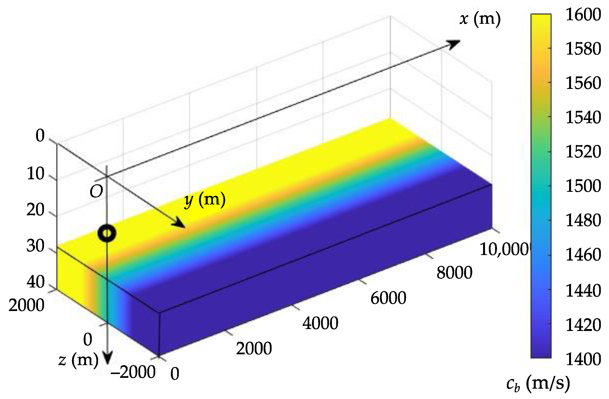
Consider the idealized shallow-water waveguide shown in Figure 1, which represents a homogeneous water layer of a constant depth $H$ over an inhomogeneous bottom halfspace. The waveguide parameters are given in

Table 1. Waveguide parameters.

Parameter	Value
Water depth $H$	28 m
Sound speed in water $c_w$	1470 m/s
Water density ${\rho }_w$	1000 kg/m3
Bottom density ${\rho }_b$	1850 kg/m3
Bottom attenuation ${\beta }_{\lambda }$	0.33 dB/λ
Transitional region width $\mathsf{\Delta }y$	2000 m

.

Let us examine sound propagation in the transitional region between an acoustically soft ($c_b<c_w$) and hard ($c_b>c_w$) bottom, as depicted in Figure 1. The bottom density ${\rho }_b$ and attenuation coefficient ${\beta }_{\lambda }$ are constant. Sound speed in the bottom varies as a piecewise-linear function of y,

$$c_b\left(y\right)=\left\{\begin{array}{c}1400\mathrm{m}/\mathrm{s},ify<-1000\mathrm{m},\left(\mathrm{soft}\mathrm{bottom}\right)\\ \left(1500+0.1·y\right)\mathrm{m}/\mathrm{s},if\left|y\right|<1000\mathrm{m},\left(\mathrm{transitional}\mathrm{region}\right)\\ 1600\mathrm{m}/\mathrm{s},ify>1000\mathrm{m},\left(\mathrm{hard}\mathrm{bottom}\right).\end{array}\right.$$

(7)

To prevent undesirable reflections, artificial absorbing layers are placed on the sides of the model domain at $\left|y\right|>2000$ m.

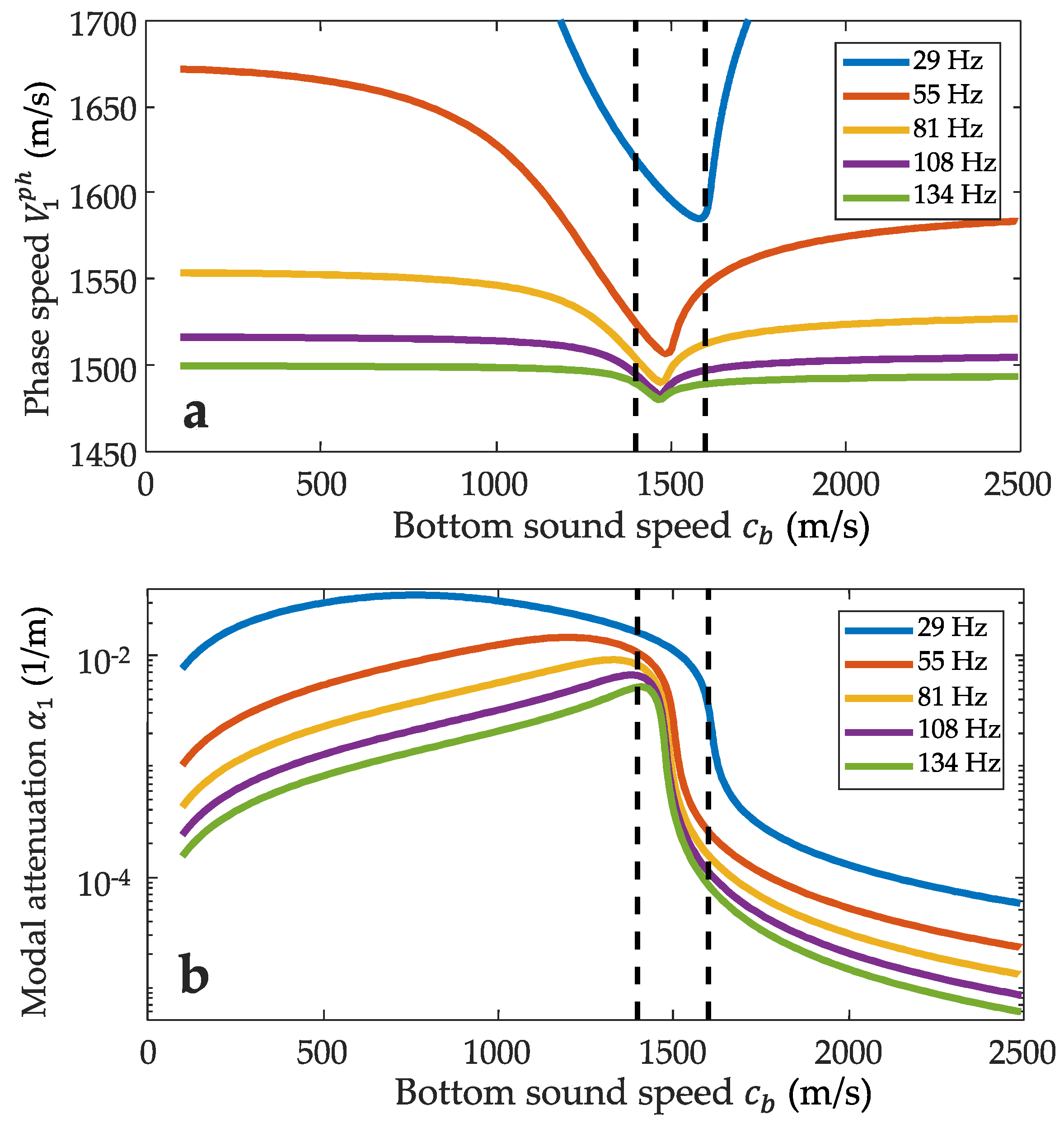
Figure 2 shows the phase speed $V_l^{ph}=\omega /q_l$ and attenuation coefficient ${\alpha }_l$ of the first mode ($l=1$) plotted vs. sound speed in the bottom $c_b$ for frequencies of 29, 55, 81, 108, and 134 Hz. For the purpose of illustration, we choose the bottom sound speed variation from 100 to 2500 m/s, which exceeds the interval of $c_b$ in the transitional region. Vertical dashed lines in Figure 2 demonstrate the boundaries of the region. Note that the phase speed $V_1^{ph}$ has a distinct minimum between these lines. The relative “depth” of the minimum is lower at a higher frequency. By placing a low-frequency sound source in the transitional region in the vicinity of the modal phase speed minimum, one can expect the effect of horizontal refraction to be pronounced. It is also important that the modal attenuation coefficient for the soft bottom is two orders of magnitude greater than for the hard bottom. The imaginary part of ${\xi }_l$ can have a large value, comparable to the real part. This feature should be carefully treated when solving Equation (4). All these remarks are also true for other normal modes ($l>1$).

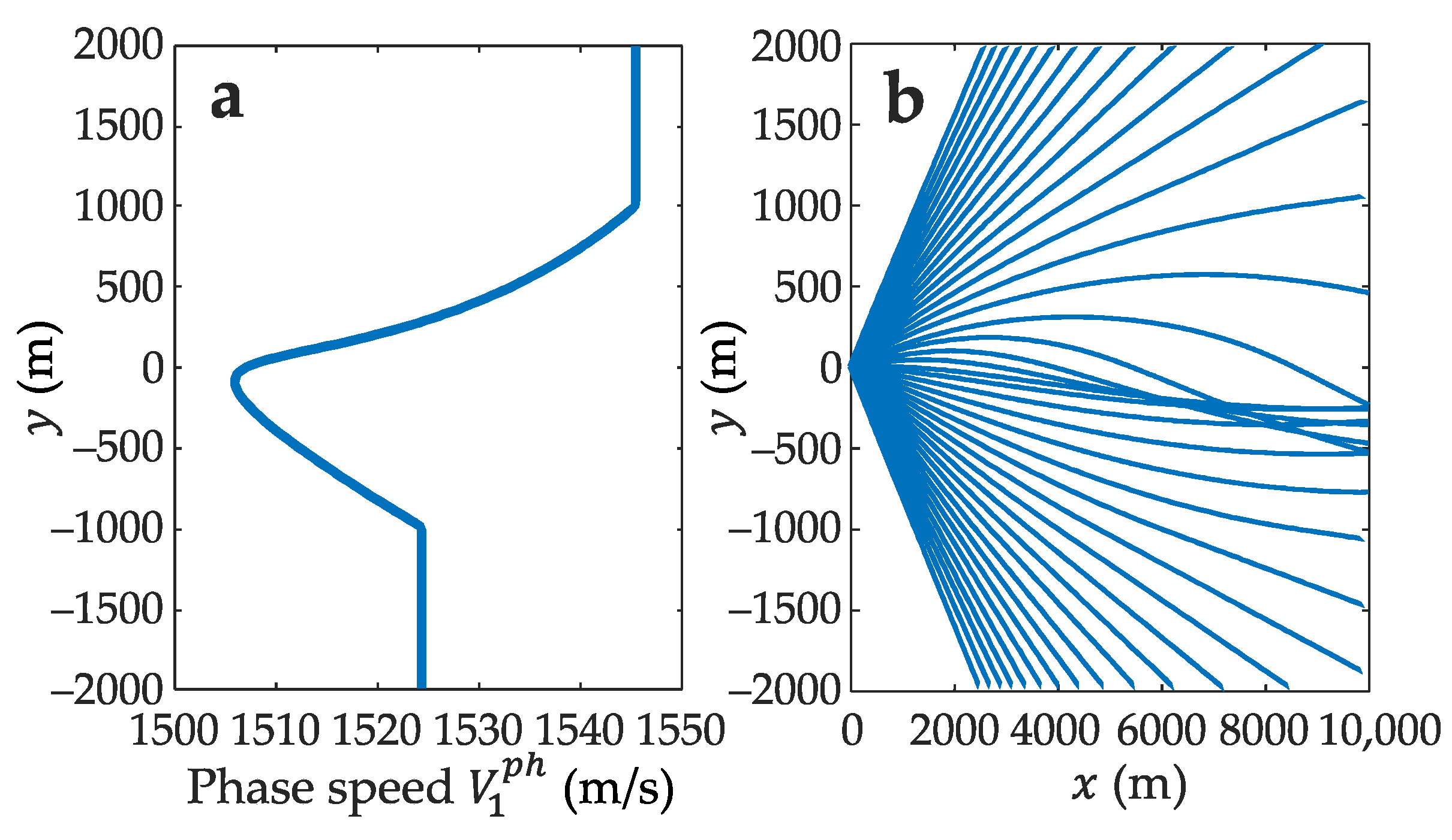
Acoustic field is calculated for a single sound source placed at the depth of $z_s=$ 15 m in the center of the transitional region, i.e., near the phase speed minimum. To demonstrate possible 3-D effects, sound propagation is simulated for a frequency of 55 Hz, at which the first mode dominates the total field. Figure 3 shows the modal phase speed $V_1^{ph}$ along the y-axis and the corresponding trajectories of modal rays calculated by a ray tracing code, BELLHOP [18], in the horizontal plane. The bending of the rays is clearly seen, which reveals the effect of horizontal refraction. The maximum angle of refraction is 7.5°. (The angle of refraction is defined as the angle between the source-receiver direction and the actual ray trajectory at the receiver.)

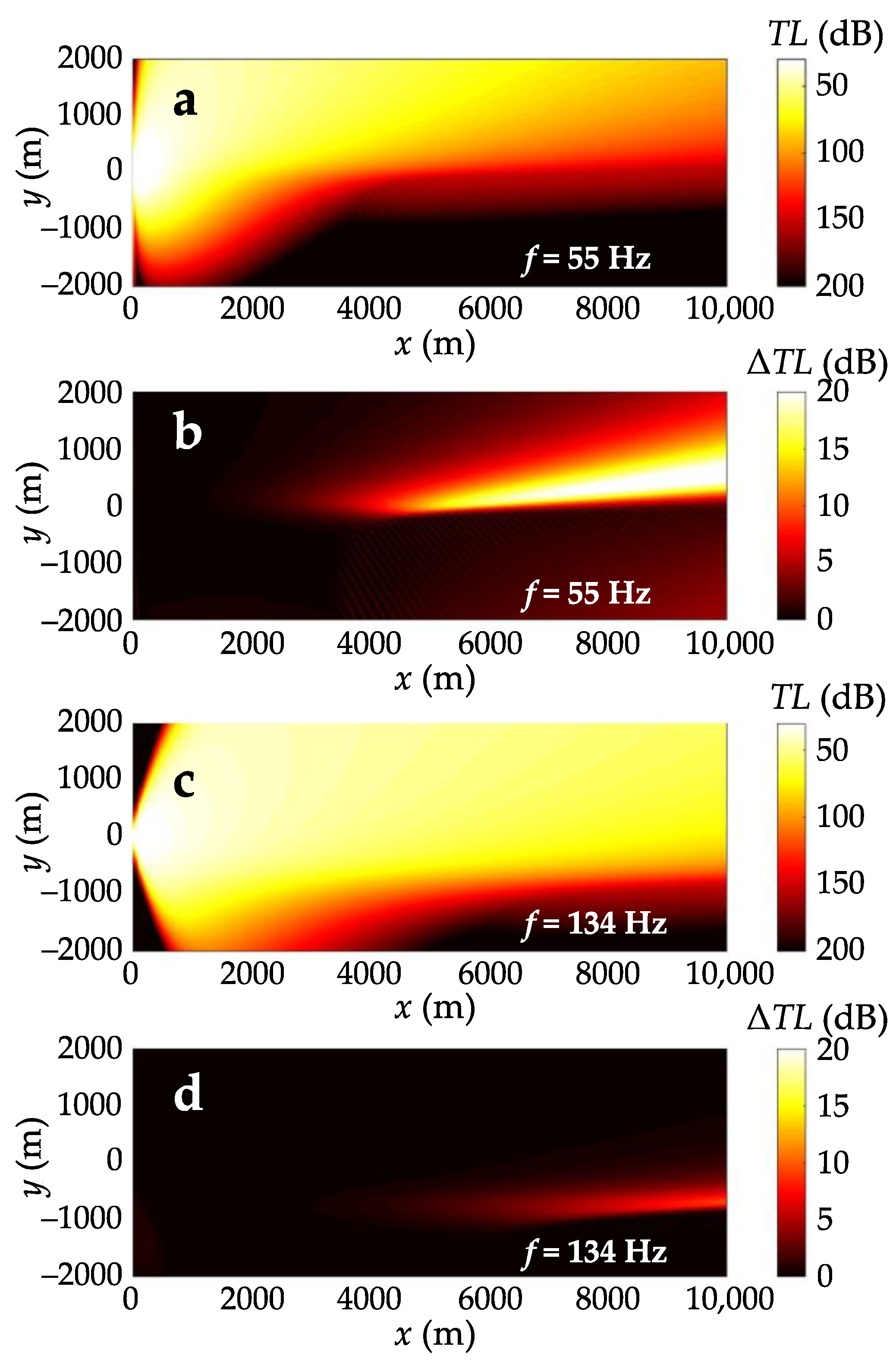
Now we estimate the effect of the refraction on the acoustic intensity distribution in the horizontal plane. Figure 4a shows the calculated 2-D transmission loss $TL$ at 55 Hz. (In this case, transmission loss of the first mode approximates the total transmission loss, $TL\approx T{L}_1$). We notice a strong azimuthal anisotropy of $TL$, that is explained by a significant spatial variability of modal attenuation, but not by the horizontal refraction itself. To highlight the effect of horizontal refraction, the transmission loss $TL$ is compared to the transmission loss $T{L}^0$ calculated using the N × 2-D approximation. As $TL$, $T{L}_0$ can also be defined by Equation (6) and Equation (1), but the modal amplitude $A_l$ in Equation (1) is found from Equation (4) with the complex wavenumber ${\xi }_l\left(x,y\right)=q_l\left(x,y\right)+i{\alpha }_l\left(x,y\right)$ replaced by $\widetilde{{\xi }_l}\left(x,y\right)=q_l^0+i{\alpha }_l\left(x,y\right)$, i.e., by keeping the spatial variability only in the imaginary part. In fact, it means that we use the adiabatic N × 2-D approximation, where mode coupling is neglected. (The proposed approach is valid only for the depth-averaged intensity estimates.) According to [12], the effects of mode coupling are secondary to those of horizontal refraction even at higher frequency, 300 Hz, in a ~80 m deep waveguide with a rough seafloor. In [19], the applicability of adiabatic approximation to depth-averaged transmission loss calculations is demonstrated for a single source in shallow water with a range-dependent bottom structure.

The spatial distribution of the transmission loss difference $\mathsf{\Delta }TL=T{L}^0-TL$ at a frequency of 55 Hz is shown in Figure 4b, which exhibits an additional insonification of the transitional region due to the horizontal refraction effect. This is explained by the fact that a curved ray, despite its longer trajectory, travels a shorter distance in the region of strong attenuation compared to a straight ray. The maximum increase in amplitude under given conditions reaches $\mathsf{\Delta }TL=$ 22 dB at 10-km range from the sound source.

In the multimodal regime at higher frequencies, the effect of horizontal refraction weakens for the first mode, but can still be exhibited in the acoustic field of other modes. However, the amplitudes of those modes are attenuated with range more rapidly than the amplitude of the first mode. Figure 4c shows the 2-D transmission loss $TL$ at 134 Hz, at which the acoustic field is effectively formed by the first three normal modes. Owing to the dominance of the first mode in the full field, the maximum difference in propagation loss between the three-dimensional case and the N × 2-D approximation does not exceed $\mathsf{\Delta }TL=$ 12 dB at 10-km range (see Figure 4d). Additional calculations for other positions of the sound source along the y-axis show that the transmission loss difference $\mathsf{\Delta }TL$ decreases to 6 dB, if the source is shifted by ±500 m relative to the initial location.

Note that the indicated effect of horizontal refraction, in principle, can be observed not only in the transitional region between an acoustically soft and hard bottom, but also, for example, in a region of hard bottom with a variable sound speed, which is close to the sound speed in water.

4. Numerical Simulations for a Real Seabed Model in the Kara Sea

The results of the previous section show the effect of horizontal refraction in an idealized waveguide of a constant depth, having the “soft bottom-hard bottom” transitional region. The key remaining question is, do such environments exist in a real ocean? Indeed, in order to observe horizontal refraction, the transitional region must be sufficiently long (at least several kilometers in length) and have a fairly regular structure.

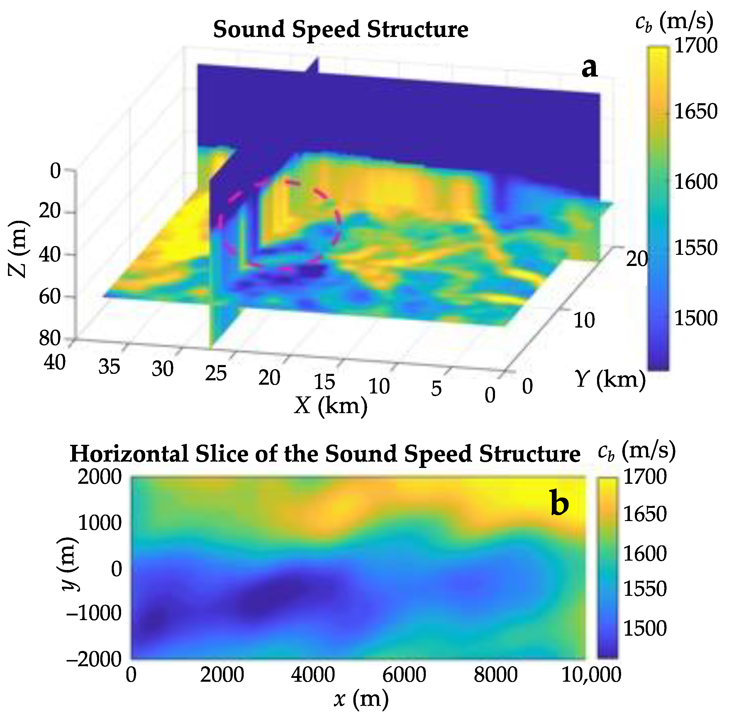
An example of a shallow-water waveguide with an inhomogeneous bottom and almost constant water depth is presented in Figure 5, which shows the sound speed structure in one of the regions of the Kara Sea. This complicated range- and depth-dependent structure is obtained by the velocity analysis of 3-D seismic survey data [11]. To study three-dimensional acoustic effects, we choose a rectangular area of the bottom, marked in Figure 5a by the dashed ellipse and shown separately in Figure 5b. The selected area is characterized by strong horizontal gradients of the sound speed in the seabed. The water depth there is equal to 28 m over the whole area.

As shown in Figure 5, the sound speed in the seabed $c_b$ varies from 1460 m/s (blue areas) to 1700 m/s (yellow areas). It is important that there exist some extended zones, where the sound speed $c_b$ in the upper sediments is approximately equal to the sound speed in water $c_b\approx c_w=$ 1460 m/s. The existence of such zones can be explained by the presence of gas-saturated or water-saturated silty sediments. The bottom density ${\rho }_b$ is assumed to be constant and equal to 1850 kg/m³, which is supported by the core sample analysis results [11]. Due to the lack of information on the sound attenuation coefficient in the seabed, its value is taken equal to 0.33 dB/λ.

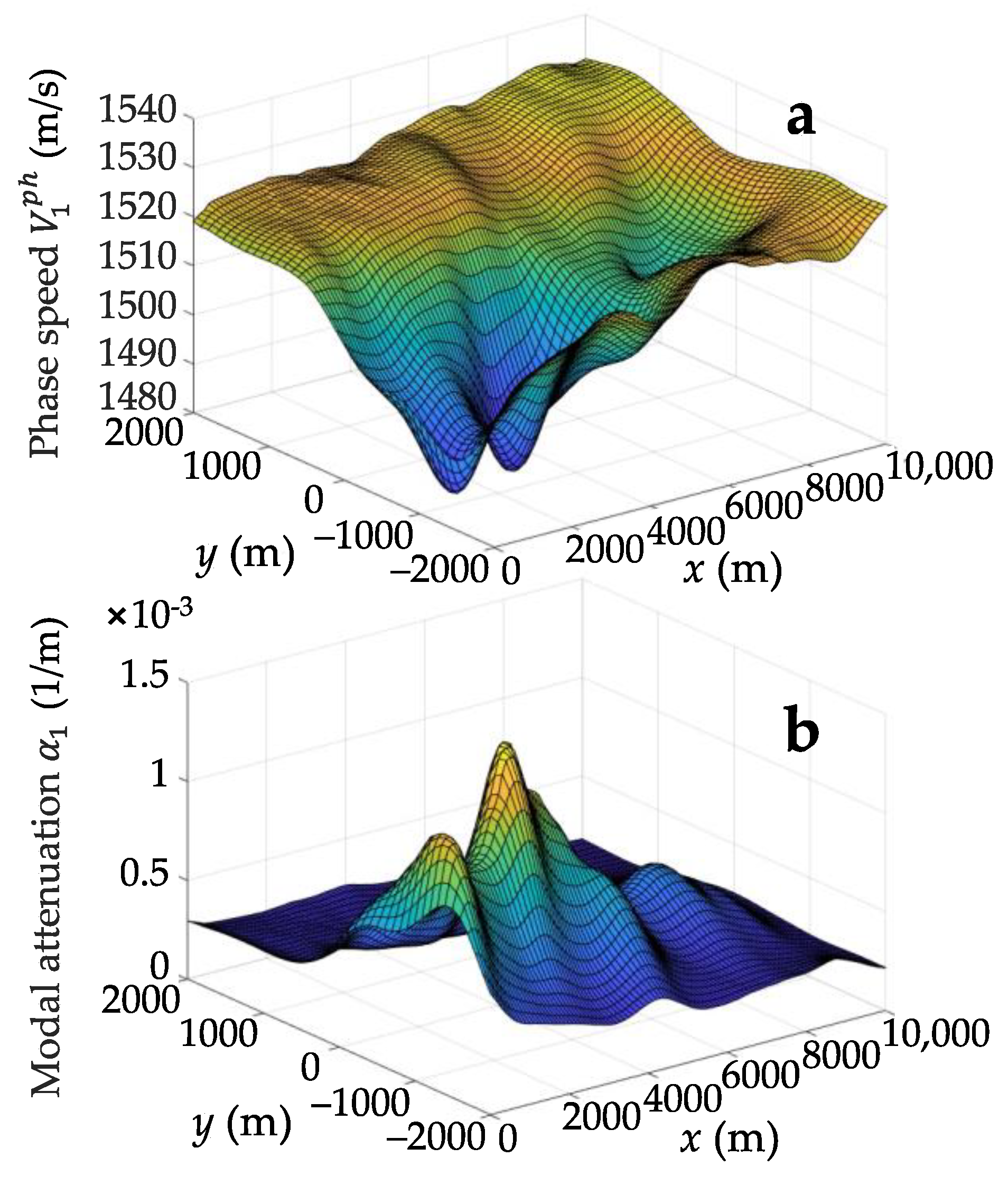
Figure 6 shows the distributions of the phase speed $V_l^{ph}$ and attenuation coefficient ${\alpha }_l$ of the first mode at a frequency of 55 Hz in the selected region. One can see a strong variability of the modal phase speed in the zone of a low sound speed in the seabed, −2000 m < y < 0 m. The maximum phase speed gradient is equal to 0.06 (m/s)/m. The same zone is also characterized by the largest values of modal attenuation ${\alpha }_l$ (up to 1.5 × 10⁻³ 1/m or 13 dB/km).

The presence of a canyon-like distribution of the phase speed shown in Figure 6a, leads to the effect of horizontal refraction, which is demonstrated in Figure 7 for a 55-Hz sound source located at (0, 0, 15 m). As in the case of the idealized waveguide model, we note the curvature of modal rays in the horizontal plane (the modal rays are depicted by white lines in Figure 7a). The maximum angle of refraction is 6°. The maximum difference in the transmission loss $\mathsf{\Delta }TL$ between the mode parabolic equation solution and N × 2-D solution, is observed in the zone of a low sound speed in the sediments, and equals to 7 dB. If the sound source is moved along the y-axis to the point (0, −1000 m, 15 m), which is in the middle of the “canyon”, the transmission loss difference increases up to 10 dB. The corresponding results at 134 Hz show the maximum difference of 4 dB. The main factor leading to the decrease of $\mathsf{\Delta }TL$ in the real simulation with respect to the simplified model is that the modal phase speed gradient is not constant along the x-axis, and its mean value is less than that in the idealized waveguide.

5. Discussion and Conclusions

The simulated depth-averaged intensity and transmission loss demonstrate the effect of horizontal refraction due to an inhomogeneous bottom structure, which can be significant even if the water column has a constant sound speed and depth. This effect is most pronounced at low frequencies in the zones, where the bottom sound speed is close to that in water.

For the realistic model of a shallow-water waveguide in the Kara Sea, the horizontal refraction at 55 Hz and 10-km range leads to the decrease in the depth averaged transmission loss by 7 dB relative to the N × 2-D approximation. In this case, the maximum angle of refraction is 6°. This value is of the same order of magnitude as in environments with a typical sloping bottom (the slope angle is ~0.5°) or intense internal waves (the amplitude is ~10 m).

The horizontal refraction associated with an inhomogeneous bottom is characterized by the following features:

• The redistribution of sound intensity in the horizontal plane is determined not only by the modal phase speed structure, but also by the modal attenuation;
• The interference of a refracted and direct modal ray is weakly exposed due to the strong difference in the modal attenuation coefficient along the rays;
• The degree of horizontal refraction strongly depends on the sound source location; the maximum effect is observed for a sound source placed above the bottom, where the sound speed is close to that in water.

The results of this work can be important, for example, for more accurate estimates of safety zone boundaries introduced for marine mammals on the Arctic shelf in the areas with a high level of anthropogenic noise. Another possible application is an array-performance prediction when estimating source bearing and range in shallow water with inhomogeneous bottom, since their estimates can be affected by horizontal refraction.