Joint Tracking of Source and Environment Using Improved Particle Filtering in Shallow Water

Abstract

Shallow water is a complex sound propagation medium, which is affected by the varying spatial–temporal ocean environment. Taking this complexity into account, the classical processing techniques of source localization and environmental inversion may be improved. In this work, a joint tracking approach for the moving source and environmental parameters of the range-dependent and time-evolving environment in shallow water is presented. The tracking scheme treats both the source parameters (e.g., source depth, range, and speed) and the environmental parameters (e.g., water column sound speed profile (SSP) and sediment parameters) at the source location as unknown variables that evolve as the source moves. To counter sample impoverishment and robustly characterize the evolution of the parameters, an improved particle filter (PF), which is an extension of the standard PF, is proposed. Two examples with simulated data in a slowly changing environment and experimental data collected during the ASIAEX experiment are utilized to demonstrate the effectiveness of the joint approach. The results show that we were able to track the source and environmental parameters simultaneously, and the uncertainties were evaluated in the form of time-evolving posterior probability densities (PPDs). The performance comparison confirms that the improved PF is superior to the standard PF, as it can reduce the parameter uncertainties. The tracking capabilities of the improved PF were verified with high accuracy in real-time source localization and well-estimated rapidly varying parameters. Moreover, the influence of different particle numbers on the improved PF tracking performance is also illustrated.

1. Introduction

Both source localization and environmental inversion are crucial issues in underwater acoustics [1,2,3,4]. Matched-field processing (MFP) combines ocean acoustics and signal processing to solve the problem of passive source localization and/or environmental inversion, yielding excellent results [5,6,7]. Despite its success, MFP is limited in certain practical applications because of its sensitivity to the mismatch between model-predicted replica fields and measurements [8]. Ideally, one class of environments can be categorized as largely range-independent and time-invariant to mitigate the disparity [2], while an environment is selected and replicas are calculated for the properties of the chosen medium. However, there is uncertainty due to fluctuations in the ocean medium, which leads to the environmental mismatch and seriously degrades the MFP performance. Typically, sound waveguide propagation in shallow ocean areas is restricted and significantly influenced by environmental parameters, such as water-column SSP [9] and seafloor parameters [10,11], including sediment sound speed, density, and attenuation, etc. Inaccurate data concerning these parameters may result in biased source localization errors.

This class of environment is significantly range-dependent and time-varying, mainly due to oceanographic variabilities and dynamics that cause the environmental parameters to evolve in time and space [2,12]. Long-term observation and wide-scale sampling is not realistic to observe all these evolving processes. For a moving source, however, the path and the ocean environment between the source and receivers change with time. These temporal variability characteristics can be merged into a tracking problem. Therefore, developing a joint tracking approach allows the environment to be estimated in real time and the source of our interest to be accurately located.

Once a tracking problem is defined as a state-space model with appropriate state and measurement equations, a suitable filter must be identified. Tracking filters, for example, the Kalman Filter family, PFs, and their extensions, have been successfully used in various tasks, such as source localization and tracking [13,14,15], environmental parameter estimation [4,16,17], geo-acoustic inversion [18,19,20], and spatial arrival time tracking [21,22]. These sequential Bayesian filters combine information on the evolution of parameters, functions that relate acoustic measurements to unknown quantities, and statistical models of random perturbations in the measurements [19]. Practical applications in ocean acoustics frequently involve complicated and fast-changing environments, the probability densities of the parameters estimated in nonstationary dynamical systems are usually non-Gaussian, and the measurement equation is thus highly nonlinear. Although the PF is an ideal algorithm for handling nonlinear/non-Gaussian systems, the well-known problem of sample impoverishment results in poor filter performance. To prevent sample impoverishment, we propose an improved PF to ensure tracking effectiveness.

The main purpose of this work was to track both source and environmental parameters simultaneously. Moreover, the goal was to both estimate the parameter values and to determine their underlying uncertainty distributions. The variations in SSP and sediment parameters were estimated jointly with source locations, rather than being calculated separately as in the existing two-step approach. To verify the feasibility of the joint tracking approach, two examples with slowly and fast-changing environments were employed.

The paper is organized as follows. In Section 2, the joint tracking approach, the state-space model, and the improved PF algorithm are described in detail. In Section 3, the standard and improved PFs source and environmental parameters tracking performance and their evolving PPDs are described using two examples. The influence of different particle numbers on the tracking performance of the improved PF is also explored. Finally, Section 4 concludes this work.

2. Particle Filter for Joint Tracking

In this section, the theory behind the joint tracking approach is summarized. Moreover, a state-space model is constructed, and the state and measurement equations are introduced. Thereafter, the steps in the improved PF algorithm are described.

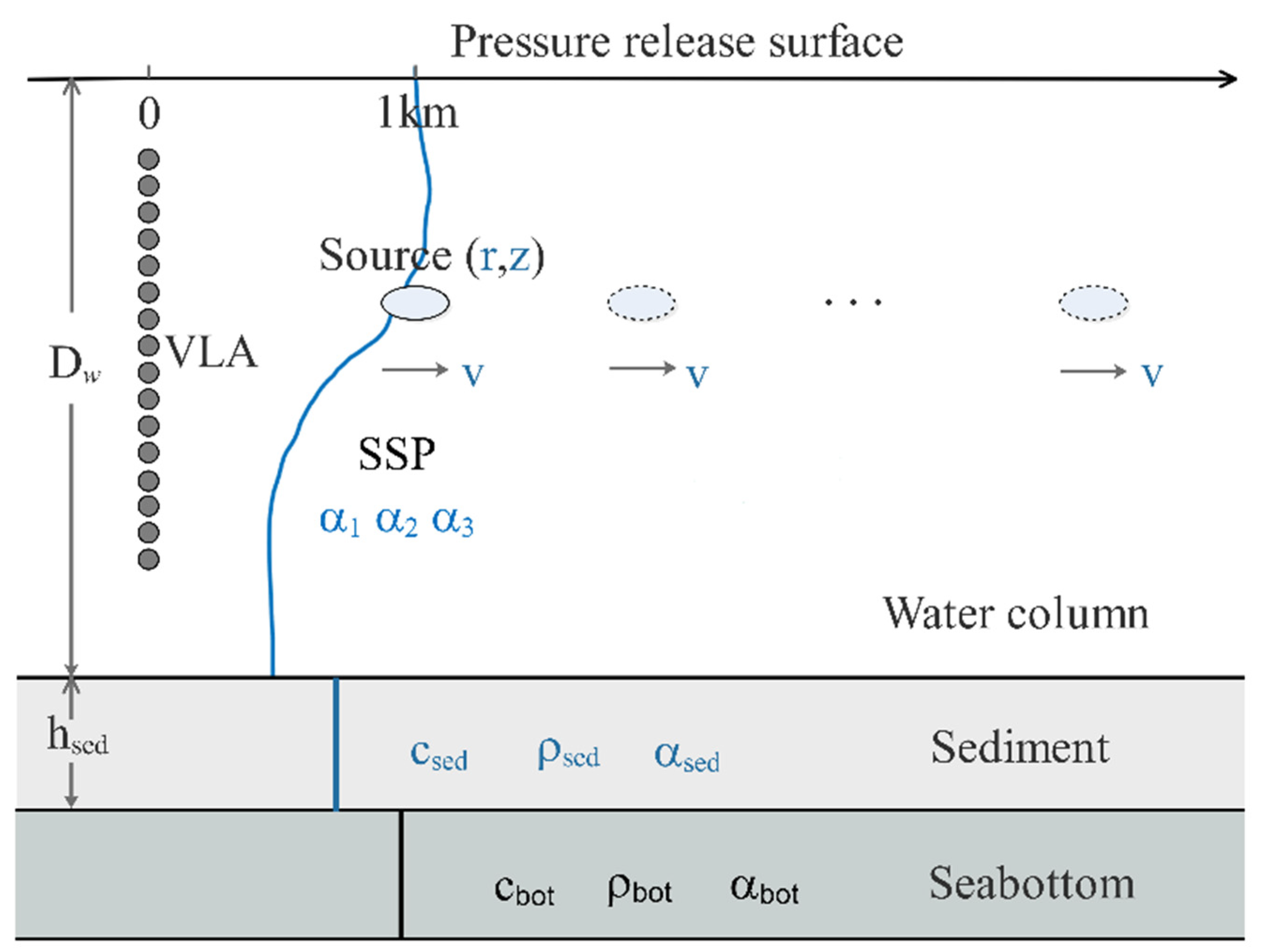
2.1. State-Space Modeling

Joint tracking of the moving source and environmental parameters requires two dynamic equations: a state equation that models both the movement of the source and the evolution of the underwater environment, and a measurement equation that relates the source location and the environmental parameters to the received acoustic data. Considering the frame $k$, two equations that define a state-space model are given as:

$$x_k=f(x_{k-1})+v_{k-1}$$

(1)

$$y_k=h(x_k)+w_k$$

(2)

where $f(\cdot )$ denotes the state transition function, and $h(\cdot )$ is the nonlinear function that relates the source and environmental parameters $x_k$ to the acoustic measurement vector $y_k$. $v_k$ and $w_k$ are the state and measurement noise vectors, respectively. The state and measurement noise covariances $Q_k$ and $R_k$ are:

$$\begin{array}{l}\mathrm{E}\left\{v_k{v}_i^T\right\}=Q_k{\delta }_{ki}\\ \mathrm{E}\left\{w_k{w}_i^T\right\}=R_k{\delta }_{ki}\\ \mathrm{E}\left\{v_k{w}_i^T\right\}=0\hspace{1em}\hspace{1em}\forall i,k.\end{array}$$

(3)

2.2. The State Equation: Moving Source and Environment Parameter Modeling

The state equation is merged from three blocks. The first is required for source tracking, and is represented as $s_k$ It is formed by the three source parameters (i.e., the source depth, the range, and the radial speed). Using a constant velocity (CV) track model for the moving source, the first block in the state equation is given by:

$$s_k={\left[\begin{array}{c}{Z}_s\\ R_s\\ v_s\end{array}\right]}_k=\left[\begin{array}{ccc}1& 0& 0\\ 0& 1& \Delta t\\ 0& 0& 1\end{array}\right]{\left[\begin{array}{c}{Z}_s\\ R_s\\ v_s\end{array}\right]}_{k-1}+\left[\begin{array}{cc}1& 0\\ 0& \Delta t^2/2\\ 0& \Delta t\end{array}\right]{\left[\begin{array}{c}{v}_d\\ v_a\end{array}\right]}_{k-1}$$

(4)

where $\Delta t$ is the update time increment (i.e., the time interval between two measurements); the random variables, $v_d$ and $v_a$, represent variations in the source depth and acceleration, respectively, which are taken as Gaussian.

The environmental parameter element is formed by SSP and sediment parameters. To limit the degrees of freedom, the SSP is often represented in terms of the empirical orthogonal function (EOF) coefficients [9], which can be obtained from the multiple conductivity–temperature–depth (CTD) measurements. As a multidimensional tracking problem, the computational complexity and estimation accuracy often depend on the number of estimated variables. In practice, the number of EOF representations can be reduced. In our previous work, it was shown that the first three EOFs are capable of representing SSP [23]. The second block is given by:

$$a_k={\left[\begin{array}{c}{a}_1\\ a_2\\ a_3\end{array}\right]}_k=\left[\begin{array}{ccc}1& 0& 0\\ 0& 1& 0\\ 0& 0& 1\end{array}\right]{\left[\begin{array}{c}{a}_1\\ a_2\\ a_3\end{array}\right]}_{k-1}+v_{k-1}$$

(5)

The third block is the state equation for the sediment parameters, including the sound speed $c_{\mathrm{sed}}$, density ${\rho }_{\mathrm{sed}}$, and attenuation ${\alpha }_{\mathrm{sed}}$, and is given as:

$$b_k={\left[\begin{array}{c}{c}_{sed}\\ {\rho }_{sed}\\ {\alpha }_{sed}\end{array}\right]}_k=\left[\begin{array}{ccc}1& 0& 0\\ 0& 1& 0\\ 0& 0& 1\end{array}\right]{\left[\begin{array}{c}{c}_{sed}\\ {\rho }_{sed}\\ {\alpha }_{sed}\end{array}\right]}_{k-1}+v_{k-1}$$

(6)

The state vector in Equation (1) includes both the source and the environmental parameters and is given by merging the three blocks mentioned above as $x_k^T=\left[s_k^T a_k^T b_k^T\right]·$$s$, $a$, and $b$ denote the parameters source, SSP, and sediment, respectively. $v$ is the state noise matrix.

2.3. The Measurement Equation: Normal Mode Propagation Model

Let $y_k$ be the acoustic pressure measured at the $k\mathrm{th}$ time frame. In Equation (2), the measurement equation is used to characterize the signal of acoustic pressure, which is received by a VLA. According to the normal mode theory, the synthetic acoustic pressure can be expressed as a general nonlinear function of the depth $Z$, horizontal range $R$, sound speed $c$ in the water column, sediment parameters, and sea bottom boundary condition (BCs).

$$y_k=h(Z, R, c_1,\cdots c_k, c_{\mathrm{sed}},{\rho }_{\mathrm{sed}},{\alpha }_{\mathrm{sed}},B{C}_S)+w_k$$

(7)

Considering the SSP is parameterized in terms of the first three EOFs, the resulting measurement equation becomes:

$$y_k=h(Z, R, {\alpha }_1,\cdots {\alpha }_k, c_{\mathrm{sed}},{\rho }_{\mathrm{sed}},{\alpha }_{\mathrm{sed}},B{C}_S)+w_k$$

(8)

where $\alpha ={\left[{\alpha }_1 {\alpha }_2 {\alpha }_3\right]}^T$, $y_k$ is the acoustic pressure measured at $k\mathrm{th}$ time frame, $h$ is the normal mode propagation model, and $w_k$ contains the measurement noise and receiver signal-to-noise ratio (SNR) in the VLA.

As mentioned above, a state–space model is formulated to track the evolving parameters.

2.4. Steps of the Improved Particle Filter Algorithm

As a result of the high nonlinearity of the measurement equation and the non-Gaussian underlying PPDs in our problem, the KF family is not feasible. As a numerical sequential Monte Carlo (MC) method, PF is suitable for tracking desired parameters and is capable of characterizing their PPDs as they evolve in time and space. Sequential importance resampling (SIR) is the most commonly used type of PF. The popularity of the SIR lies in the simplicity of the selection of transition prior as the sampling density, i.e., $p\left(x_k|x_{k-1},y_k\right)=p\left(x_k|x_{k-1}\right).$ Although resampling has the ability to reduce degeneracy, it causes sample impoverishment, which can be a problem for the standard SIR PF algorithm and results in poor filter performance, especially for low process noise systems. Because the resampling stage creates many exact replicas of high likelihood particles, it is possible to lose sample diversity and validity as the filter progresses [24].

To prevent sample impoverishment, an improved SIR PF is proposed. The algorithm uses the likelihood optimization function to guide the importance sampling particles to the high likelihood regions, which ensures resampling diversity. Hence, the key step of the improved algorithm is the likelihood calculation.

Following Equation (2), i.e., the additive complex Gaussian noise for step k, the likelihood function is of the form:

$$\begin{array}{l}L\left(x_k\right)=e^{L_0^{\prime }\left(x_k\right)-\max L_0^{\prime }\left(x_k\right)}\\ L_0\left(x_k\right)=\ln \frac{1}{{\left(\pi w_j\right)}^{n_h}}-\frac{{\Vert y_k-h\left(x_k\right)\Vert }^2}{w_j}\end{array}$$

(9)

where $n_h$ is the hydrophone number of VLA and $w_j$ is the noise variance.

A single iteration at step $k$ of the SIR has three stages:

Prediction: starting with a set of particles from the previous state ${\left\{x_{k-1}^i\right\}}_{i=1}^{n_p}$, where $n_p$ is the particle number, a new set of predictions ${\left\{x_k^i\right\}}_{i=1}^{n_p}$ is created by sampling from the transitional density $p\left(x_k|x_{k-1}\right)$. This is achieved by propagating each particle through the state Equation (1) together with the random state noise $v_k$.

Updating: the predictions in the previous step are updated using the acoustic pressure data $y_k$ at the current step $k$, and the normalized weight $w_k^i$ of each particle is computed via:

$$w_k^i=L\left(x_k^i\right)/{\displaystyle \sum {}_{j=1}^{N_p}}L\left(x_k^j\right)$$

(10)

where the likelihood function $L\left(x_k\right)$ is calculated by Equation (9). Let the set of particles and their weights ${\left\{x_k^i, w_k^i\right\}}_{i=1}^{N_p}$ characterize the posterior density, and we have:

$$p\left(x_k|y_1\cdots y_k\right)\approx {\displaystyle \sum _{i=1}^{n_p}{w}_k^i\delta \left(x_k-x_k^i\right)}$$

(11)

Resampling: this stage redistributes samples so that the number of samples in a region of state space is proportional to the posterior density of that region. Resampling generates particles according to the weights of the parent particles $w_k^i$, with more particles generated from high probability particles than low ones. All particle weights are now equal to $1/N_p$. The PPD is given by:

$$p\left(x_k|y_k\right)=\frac{1}{N_p}{\displaystyle \sum _{i=1}^{n_p}\delta \left(x_k-x_k^i\right)}$$

(12)

The minimum mean square error (MMSE) estimate that calculates the expected value of the state vector is given as:

$${\widehat{x}}_k=\frac{1}{N_p}{\displaystyle \sum _{i=1}^{N_p}{x}_k^i}$$

(13)

More details can be found in [24]. The improved SIR PF algorithm is used throughout this work. Hereafter, “the improved PF” refers to the improved SIR PF.

3. Examples and Discussion

This section is composed of two examples. The first is a synthetic tracking simulation in a slowly changing shallow water environment with small variations in environmental parameters. In the simulation, the standard and improved PFs are not only compared with each other, but ways to track parameter uncertainties as PPDs are also demonstrated. The second tracking example analyzes data collected during the ASIAEX experiment. In this example, both the source and environmental parameters in various time intervals changed fast, which was used to test the performance of the improved PF in the case of a fast-changing environment.

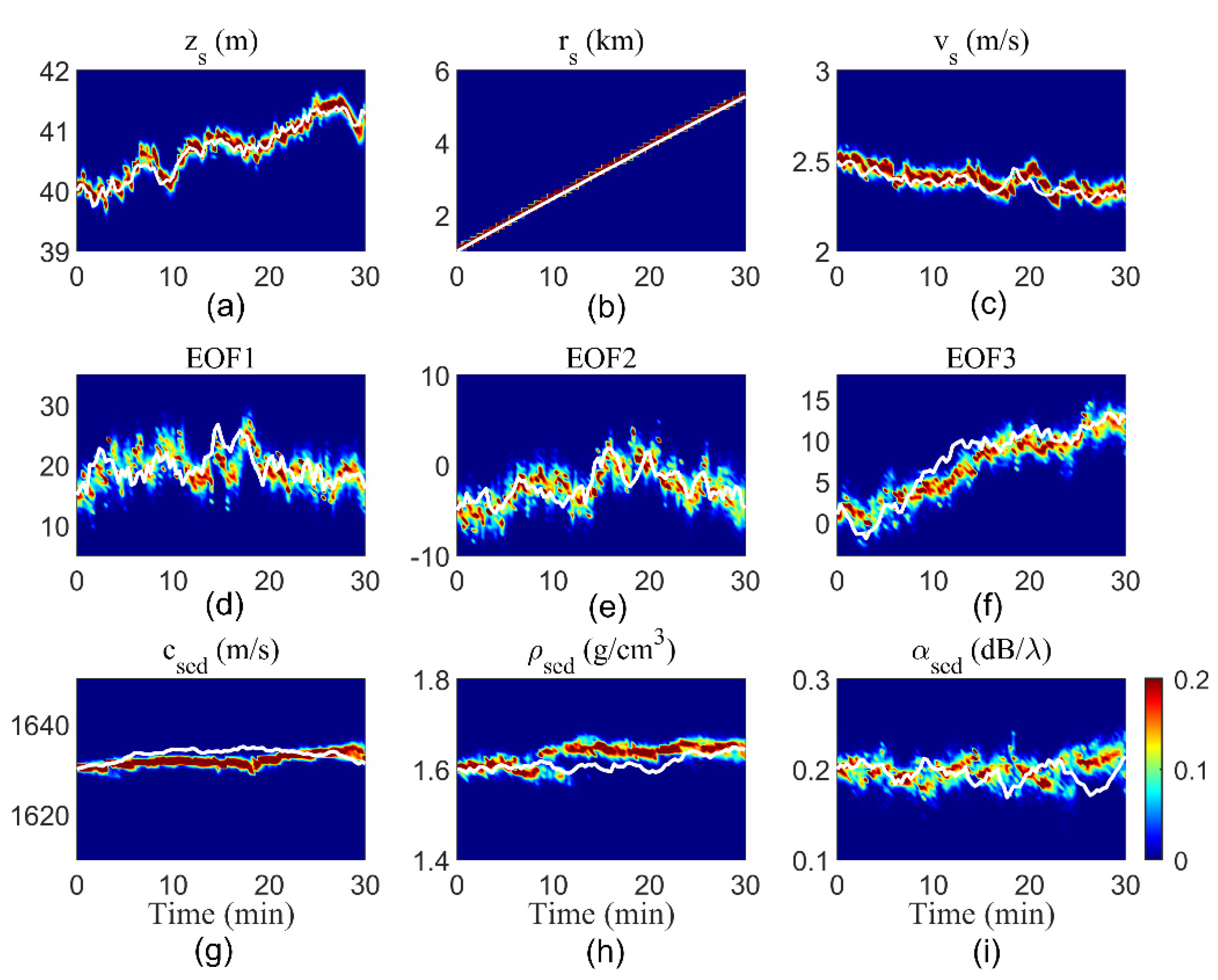
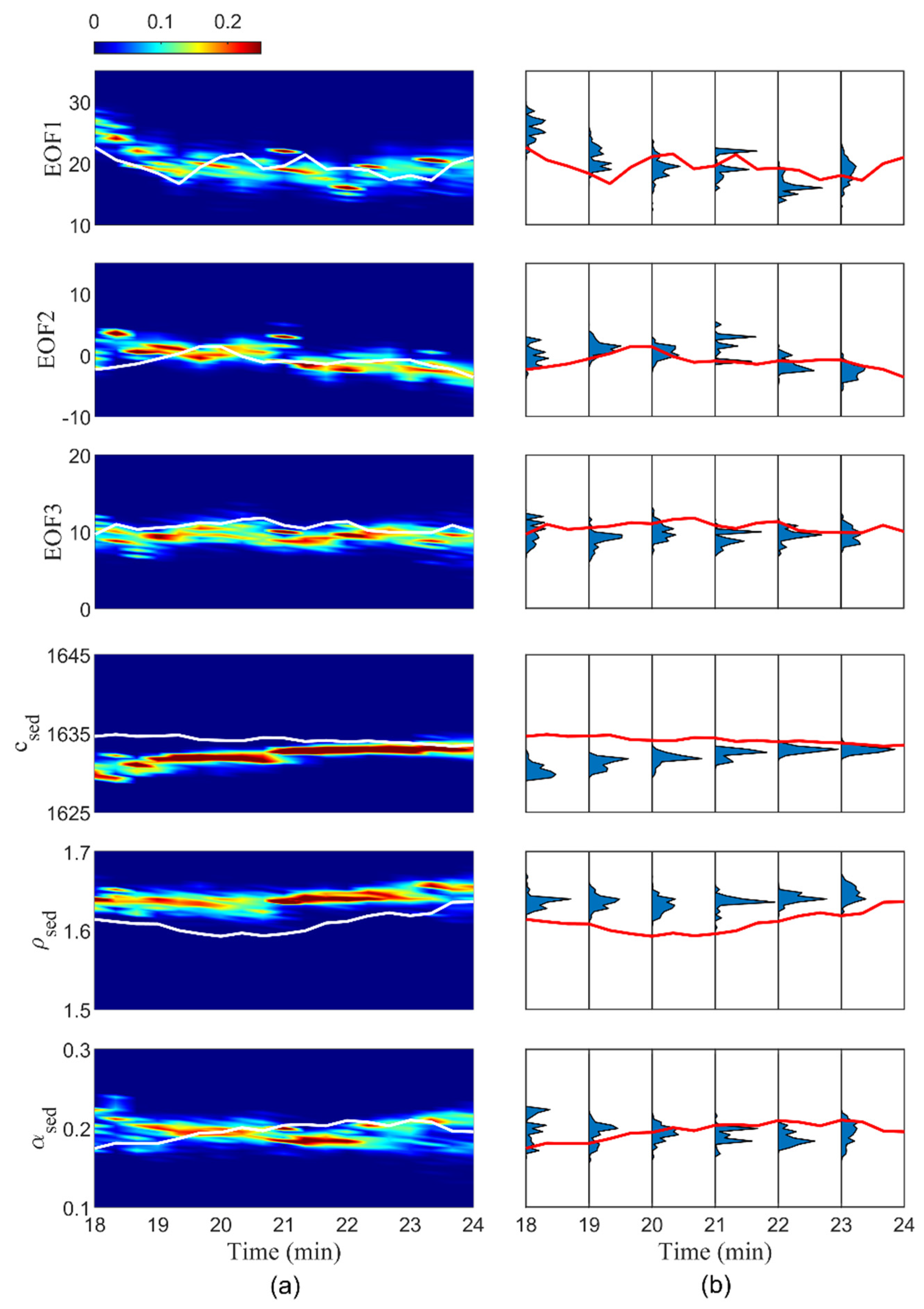
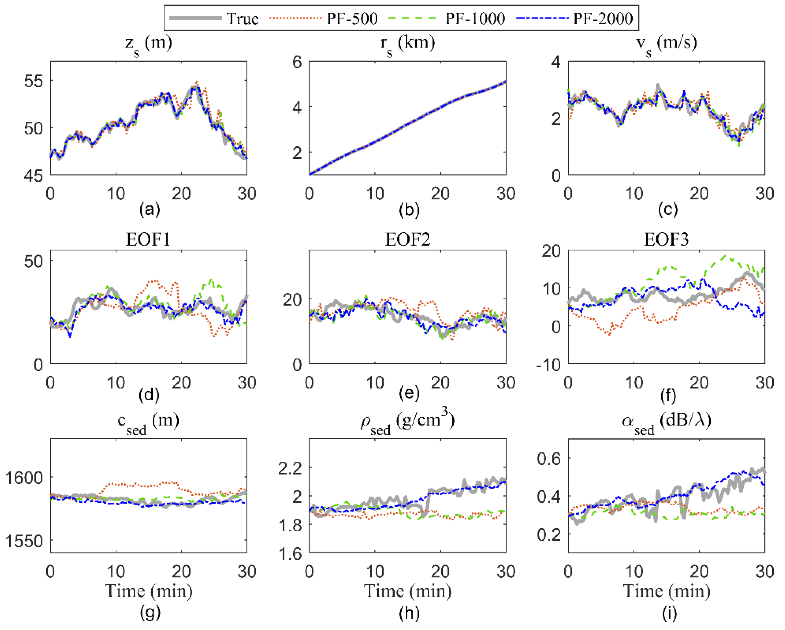
3.1. Simulated Data in a Slowly Changing Environment

To synthesize the acoustic pressure data used in the measurement equation, a forward propagation model was used, as is shown in Figure 1. It consisted of 106 m deep water, a 3 m thick sediment layer, and a bottom layer. The bottom was assumed to be a homogenous half space with a constant sound speed of 1887 m/s, a density of 2.17 g/cm³, and an attenuation of 0.05 dB per wavelength. The simulation was set up with a fixed VLA and a moving source in the range-dependent shallow water. The VLA was configured with 16 elements deployed from 15 to 75 m in depth, paced 4 m apart. The initial position of the source was at 40 m in depth and 1 km in range. A frequency of 400 Hz was selected. The source was towed and had a 90-step (k = 1, 2…, 91) movement at a speed of 2.5 m/s, resulting in a total track length of 30 min. The SSP and sediment parameters changed with time as the source moved, representing the changing average values of SSP and sediment parameters between VLA and the new source position.

In this tracking simulation, the sediment parameters did not vary much. The largest variation came from the water column SSP, which is known to fluctuate significantly with time. As mentioned in Section 2.3, the SSP was tracked by three tracking EOFs. All the simulation parameters, constants, nine state variables, and their start values $x_0$ (prior standard deviations $P_0^{1/2}$ and state noise deviations $Q_k{}^{1/2}$) are given in

Table 1. Environmental and simulation parameters for Example 1.

Environmental Parameters
		State Variables
Constants			$\mathbf{x}$	${\mathbf{x}}_0$	${\mathbf{P}}_0^{1/2}$	${\mathbf{Q}}_{\mathit{k}}^{1/2}$
$D_{\mathrm{w}}$	106 m	Source	$z_s$ (m)	40	0.1	0.1
$h_{\mathrm{sed}}$	3 m		$r_s$ (m)	1000	2	0.0134
$c_{\mathrm{bot}}$	1887 m/s		$v_s$ (m/s)	2.5	0.2	0.0024
${\rho }_{\mathrm{bot}}$	2.17 g/cm3	Water	EOF1	15	1.5	1.5
${\alpha }_{\mathrm{bot}}$	0.05 dB/${\lambda }^{}$		EOF2	−5	0.9	0.9
			EOF3	1	0.6	0.6
		Sediment	$c_{\mathrm{sed}}$ (m/s)	1630	0.2	0.2
			${\rho }_{\mathrm{sed}}$ (g/cm3)	1.6	0.005	0.005
			${\alpha }_{\mathrm{sed}}$ (dB/$\lambda$)	0.2	0.005	0.005
Simulation parameters
Source frequency		400 Hz	SNR		29 dB
Receiver type		16-VLA	Tracking length		30 min (k = 91)
First/last hydrophone depth		15/75 m	Sampling interval $\Delta t$		20 s

. For the convenience of calculation, we assumed that both additive noise terms $Q_k$ and $R_k$ were represented by the Gaussian PDFs. The adiabatic normal mode propagation model was selected to adequately compute the acoustic field by inputting the source and environmental parameters into KRAKENC [25].

According to the state–space model formulated in Section 2, the state consisted of nine variables (including source depth, range, and speed), three EOFs of the water column SSP, and sediment sound speed, density, and attenuation coefficient. Two PFs were used to simultaneously track these nine parameters. It is known that a higher approximation accuracy can be obtained for the posterior distribution with a larger number of particles. To ensure the tracking accuracy, the number of particles was set to n_p = 500. All particles were propagated through the state equation, updated via the measurement equation, resampled, and then the evolution of state variables was estimated.

First, the standard PF was used for tracking. The evolution of the 1-D marginal posterior densities for the nine parameters is given in Figure 2. The evolving PPDs were obtained in terms of the normalized histograms of particles; hence, they contained information about uncertainty in the estimation of the source and environmental parameters. Here, using the same settings, the improved PF was implemented, and the tracking results are shown in Figure 3.

The plots in the first row belong to the source parameters. Along the 30 min trajectory, the source depth oscillated between 39 and 42 m, while the source moved from 1 to 5.5 km in the horizontal range. For all three source parameters, the 1-D marginal PPDs followed the true trajectories. The depth and range of the source were tracked accurately with small deviations. The variation in the radial speed was also well tracked. Both PFs were able to track the source parameters successfully.

The environmental parameter tracks are in rows 2–3. The SSP and sediment parameters were taken as range-dependent and they changed with time as the source moved. For the three EOFs, PF roughly tracked the evolution of the true trajectories. However, the sample impoverishment and blind prediction of PF resulted in large tracking errors in certain rapidly changing regions. Although SSPs in the water column were expected to evolve slowly in general, there were rapid perturbations in sound speed in certain regions of the true environment. The perturbations resulted in larger variations in the EOFs, which exceeded the statistical values assumed for the random walk, and resulted in a model mismatch. As a result of the combination of a large state variation and inadequate particle number, a sample impoverishment problem may have occurred in several iterations. Along with the tracking in the third row, the sediment sound speed remained between 1628–1636 m/s, a density of 1.59–1.65 g/cm³, and an attenuation of 0.16–0.22 dB/${\lambda }^{}$. The PPDs became non-Gaussian, and the plots $c_{\mathrm{sed}}$, ${\rho }_{\mathrm{sed}}$, and ${\alpha }_{\mathrm{sed}}$ were less well-tracked than other parameters. The main reason for the tracking results was the lower sensitivity of the sediment parameters to the acoustic field. This is in agreement with the sensitivity analysis in [14].

As expected, the improved PF is superior to standard PF in terms of joint tracking performance. For the improved PF, the parameters were tracked accurately with small deviations from the true values. This is especially obvious from the tracking trajectories when the state variables change rapidly.

The joint tracking errors can be evaluated by the root mean square error (RMSE) metric, which essentially calculates the difference between the true values and the estimated parameters from the PFs. To quantify the average tracking performance and integrate across these errors to provide a single number, the following time-averaged RMSE is defined as:

$$\mathrm{TARMSE}=\frac{1}{k_2-k_1+1}{\left[{\displaystyle \sum _{k=k_1}^{k_2}\frac{{\left({\widehat{x}}_k-x_k\right)}^2}{k_2-k_1+1}}\right]}^{1/2}$$

(14)

where $t$ is the time interval; ${\widehat{x}}_k$ and $x_k$ denote the true and estimated parameters at time index k, respectively; and TARMSE is the time-averaged RMSE calculated for the time interval $\left(k_1, k_2\right)$. The total track length was 30 min, and the time interval was set as (1, 91) for computations. Equation (15) was used to calculate the performance improvement of the improved PF with respect to the PF, and to compare the performance metrics in

Table 2. Performance comparison for Example 1.

Parameter	zs (m)	rs (m)	vs (m/s)	EOF1	EOF2	EOF3	csed (m/s)	ρsed (g/cm3)	αsed (dB/λ)
TARMSEPF	0.0091	0.1994	0.0029	0.244	0.1537	0.2123	0.3490	0.0035	0.0020
TARMSEimpro.-PF	0.0076	0.1378	0.0026	0.2076	0.116	0.1558	0.2042	0.0018	0.0012
% Impro.	16	31	10	15	25	27	42	49	40

. It was confirmed that the improved PF did well in terms of error variance reduction in terms of tracking all nine parameters. It exhibited an average of a 28.3% improvement over the PF. Note that the sediment parameters exhibited more than a 40% improvement and were closer to the evolution of the true values than the PF tracking results.

$$\mathrm{Impro}.=\frac{{\mathrm{TARMSE}}_{\mathrm{PF}}{-\mathrm{TARMSE}}_{\mathrm{improved}-\mathrm{PF}}}{{\mathrm{TARMSE}}_{\mathrm{PF}}}$$

(15)

In the above simulations, the standard and improved PFs simultaneously tracked the source and environmental parameters and their uncertainties were evaluated in the form of time-evolving marginal PPDs. This ability enabled the moving source to be located in real time.

For moving source localization, we investigated the performance of the filters by computing and plotting the posterior source depth-range probabilities. Both PFs tracked the source depth and range for all t. The evolutions of the 2-D PPD of the source at three time steps are shown in Figure 4. The source localization results at 3.3, 13.3, and 28 min are given in

Table 3. Source localization results.

$\mathit{t}$ (min)	Method	${\mathit{z}}_{\mathit{s}} \left(\mathbf{m}\right)$	${\mathit{r}}_{\mathit{s}} \left(\mathbf{m}\right)$	${\mathit{v}}_{\mathit{s}} (\mathbf{m}/\mathbf{s})$
3.3	True value	40.03	1492.8	2.45
	PF	40.19	1493.4	2.44
	Improve-PF	40	1492.2	2.46
13.3	True value	40.79	2933.2	2.42
	PF	40.55	2934.2	2.40
	Improve-PF	40.72	2933.4	2.41
28	True value	41.35	4997.5	2.32
	PF	41.37	5001.0	2.28
	Improve-PF	41.33	4999.2	2.31

.

It was clearly observed that the improved PF enabled the source to be tracked accurately in terms of range and depth with reduced errors. The improved PF only exhibited errors of 0.02–0.07 m, 0.2–1.7 m, and 0.01 m/s in the three mid-tracks for the source depth, range, and speed, respectively. Even after the full track length of 30 min, the error terms remained at 0.07 m, 1.4 m, and 0.004 m/s. Therefore, the real-time location was realized at any given t, and, thus, the improved PF is a significant improvement over the standard PF in terms of source localization accuracy.

As the tracking time progresses, the PFs utilize both current data and the estimated previous parameter results to update the parameter in the next step. This enabled us to obtain histograms of particles that represent the marginal PPDs of the parameters estimated in any period of time. Although the environmental parameters change gradually between the source and receiver, there are sudden jumps in certain periods. A representative 6-min tracking duration was selected, in which the parameters changed rapidly. The results from 18 to 24 min are given in Figure 5 and Figure 6 for the standard PF and improved PF, respectively. The marginal PPDs with six-time-step increments are plotted at every 1-min interval on the right.

The PPDs of the standard PF demonstrate a larger uncertainty as compared to the improved PF. Furthermore, the EOFs and sediment parameters had non-Gaussian PPDs, and the peak values did not coincide with the true trajectories at the corresponding time intervals. For the improved PF, all the estimated parameters generally followed the true trajectories. The variations in three EOFs were captured throughout the track, and each has a sharp PPD with a high probability of the true value. The estimations of sediment sound speed, density, and attenuation were similarly improved, closely following the true values. Therefore, the comparison results again show that the improved PF outperformed the standard PF, especially in the rapidly varying environment.

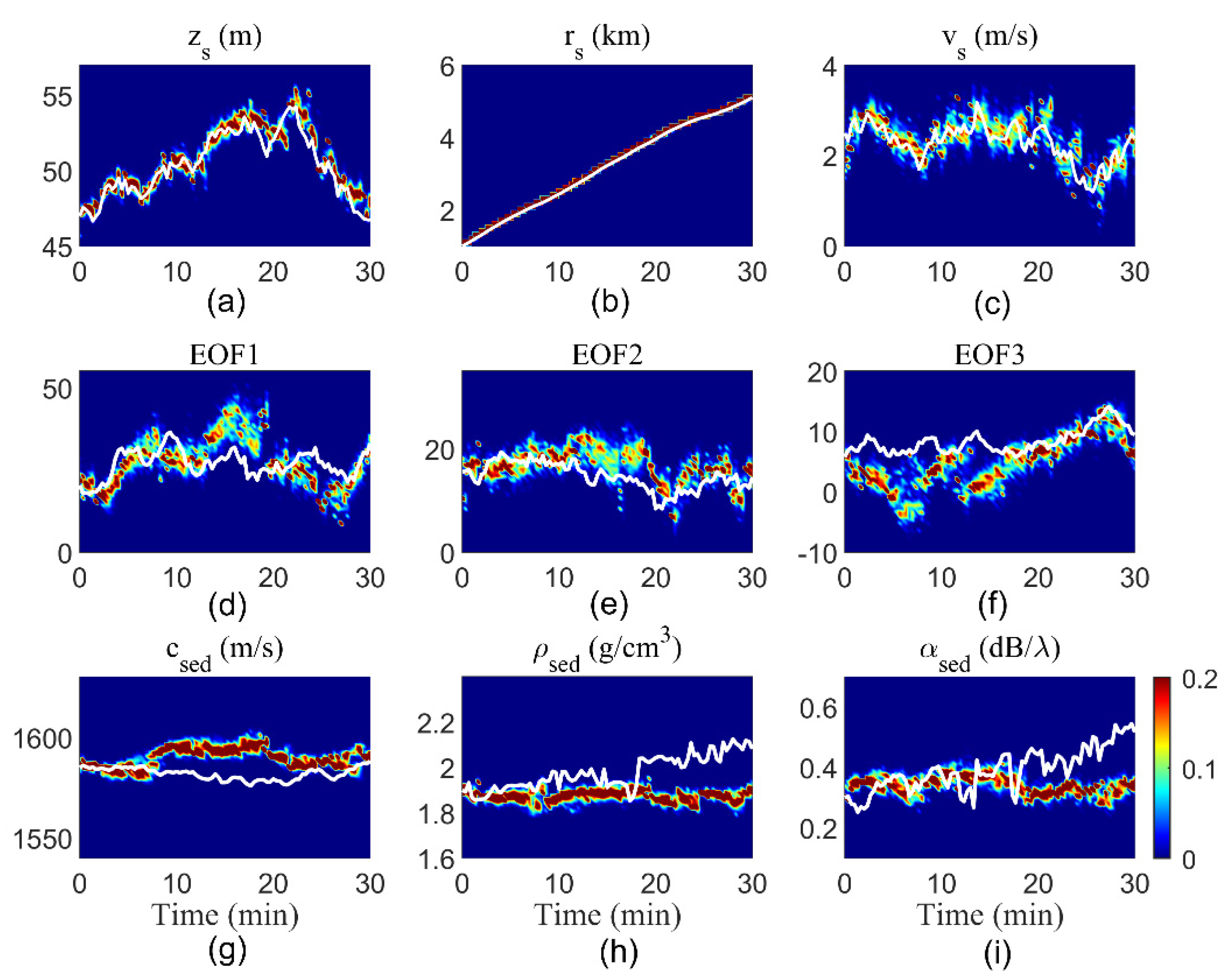
3.2. ASIAEX Experiment Data in the Fast-Changing Environment

As mentioned above, the improved PF is illustrated to capture the rapid variation in environmental parameters. To test the performance of the improved PF in the case of a fast-changing environment, the data obtained from the core measurements of the ASIAEX 2001 Experiment were used [26]. The ASIAEX consisted of two major experiments; in this work, we concentrate on the ECS part, which helps contribute to a deeper understanding of ocean acoustic propagation and geo-acoustic inversion in shallow water. A key phase in the experiment was from 2–6 June 2001. During this phase, variation caused by the fast-changing waves was evident, and high winds resulted in increased water column mixing. In view of this variability, the measurements were specifically designed to capture the acoustic effects of changing sea state conditions. The experimental site is depicted in [26]. The EOFs were calculated from the measured SSPs. Within a 30-km radius, sediment cores were collected. The seabed was relatively flat, with an approximate depth of 105 m. Since the acoustic field has little sensitivity to bottom parameters, their influence on the measured field was negligible; therefore, herein, the seabed was modeled as a fluid. The source was initially placed at a depth of 50 m and a range of 1 km, and then moved away from the VLA at a rough speed of 2.5 m/s. Unlike the towed source in the first example, the source used here could also move in the depth plane. A signal frequency of 400 Hz and a lower SNR of 22 dB were used to calculate the acoustic field. The environmental model given in Figure 1 was adopted here, with the same VLA configuration.

Before implementing joint tracking, the signal at time index k = 0 was used to carry out matched-field inversion to obtain prior information about the environmental parameters, and the results were used as initial vectors in joint tracking [6]. The prior standard deviations $P_0^{1/2}$ and state noise deviations $Q_k{}^{1/2}$ of these parameters are given in

Table 4. ASIAEX: improved-PF initiation.

$\mathbf{x}$	${\mathbf{P}}_0^{1/2}$	${\mathbf{Q}}_{\mathit{k}}^{1/2}$
$z_s$ (m)	2	0.5
$r_s$ (m)	50	2
$v_s$ (m/s)	0.8	0.2
EOF1	4	2
EOF2	2.4	1.2
EOF3	1.6	0.8
$c_{\mathrm{sed}}$ (m/s)	2	1
${\rho }_{\mathrm{sed}}$ (g/cm3)	0.02	0.02
${\alpha }_{\mathrm{sed}}$ (dB/${\lambda }^{}$)	0.02	0.02

. The selection of suitable noise covariances is essential in order to tune the PF performance. It can be seen from [14] that the selection of $Q_k$ is a trade-off between how much we trust the evolution model given in the state equation and how noisy an estimate we want. Note that the greater the prior and state noise deviation, the more likely the filter is qualified for tracking rapid changes in the state parameters, and, the greater the risk of divergence. Therefore, in this example, the initial parameters were selected to have a larger $Q_k$ and a relatively broad Gaussian distribution with $P_0^{}$. The improved PF was used throughout the following work. To simplify the expression, all the PFs mentioned below refer to the improved PF. The initial default number of particles was still 500.

The tracking results of the ASIAEX experiment are shown in Figure 7. Although the evolution of the source changed rapidly, it was accurately captured. However, the divergence phenomenon inevitably occurred, especially for the evolutions of EOFs and three sediment parameters. As the parameters started to evolve rapidly, the PF was unable to follow, and larger errors began to appear in the corresponding PPDs. There are many causes of tracking divergence, such as filter limitations, errors in the forward model, and incorrect assumptions about the state and measurement noise [18]. The rapidly varying environment is an important factor, as the parameter values of the current measurement may change significantly from the previous values. A large $Q_k$ can capture sudden changes in the state, but a large noise term will make the tracking diverge. A PF of 500 particles performs poorly due to the insufficient number of particles used in tracking. Therefore, the number of particles needs to be increased; if more sampling particles cover the high-likelihood area of parameters, a more accurate PPD characterization can be obtained.

Each of these nine parameters was tracked by the PFs using 500, 1000, and 2000 particles designated by PF-500, PF-1000, and PF-2000, respectively. The PFs tracking results are given in Figure 8 along with the true trajectories. Increasing the number of particles initially provided a large PF performance improvement. Although the tracking results of PF-1000 improved, the divergence still existed. The third filtering strategy was performed using a PF-2000. It was confirmed that PF-2000 outperformed the PF-500 and PF-1000 over the whole tracking period. However, no matter which kind of PF was used, the source parameter tracking results were always robust. Since the acoustic field was not that sensitive to the sediment sound speed, density, or attenuation, the PF-500 failed to track them, and they were relatively poorly estimated. The PF-2000 was able to maintain tracking, albeit with some errors.

After the quantitative comparison, PF-2000 outperformed the two other PFs in terms of TARMSEs for all the parameters (see

Table 5. TARMSE of improved-PFs for ASIAEX tracking results.

Filter	zs (m)	rs (m)	vs (m/s)	EOF1	EOF2	EOF3	csed (m/s)	ρsed (g/cm3)	αsed (dB/λ)
PF-500	0.0534	0.5956	0.0204	0.589	0.2707	0.4218	0.8018	0.0082	0.0119
PF-1000	0.0304	0.2608	0.0171	0.4217	0.1867	0.4027	0.2874	0.0055	0.0098
PF-2000	0.0244	0.1838	0.0161	0.263	0.171	0.3374	0.2722	0.0045	0.0028

). The desired accuracy in tracking results is one of the major factors in selecting the number of particles. However, for a tracking algorithm, it is necessary to take the computational cost into account. An upper limit for the particle number is determined by the maximum number that can be processed with limited computational resources, which is especially important for real-time filtering algorithms. Although not given here, the influence of different particle numbers on PF tracking accuracy and computational cost is demonstrated and evaluated in our previous work [27].

In practice, sea state conditions are complicated and changeable. This causes the state variable to vary in a way that is not consistent with the state model, with rapid changes occurring. Under such circumstances, successful tracking requires a filtering algorithm to be able to capture the state variations in time. The state noise, particle number, and computational cost need to be carefully selected. These tradeoffs can make selection a practical challenge.

4. Conclusions

In this paper, a joint tracking approach for a moving source and environmental parameters in shallow water is presented. The source (e.g., source depth, range, and speed) and environmental (e.g., water column SSP and sediment parameters) parameters were simultaneously tracked by assimilating the measurements of the acoustic field on a VLA into standard and improved PFs. The simulated slowly changing environment and the ASIAEX ECS 2001 experiment were used to test the efficiency of the tracking schemes.

Both PFs were able to provide real-time, continuously updated tracking of the parameters and their underlying probability densities in the form of a time-evolving PPD. A comparison of the simulation results confirmed that the improved PF was superior to the PF. The tracking capabilities of the improved PF are demonstrated in its higher source localization accuracy and robust environment tracks in the period when the parameters changed rapidly.

The influence of different particle numbers on the improved PF tracking performance was also illustrated. It should be noted that increasing the particle number provides a large tracking improvement, whereas the computational cost is greatly increased. Additionally, larger state noise improves sample diversity to enable the filtering to capture state variables in a fast-changing environment, but this increases the risk of divergence. Therefore, the selection of state noise, particle number, and computational cost is always a tradeoff and should be further explored.

Our approach has practical value in ocean acoustic applications. It enables spatial–temporal tracking of parameters and their underlying uncertainties, making the approach a natural extension of target localization and geo-acoustic inversion techniques. For signal processing in complex and variable sea states, the introduction of the improved PF may be a promising technique for nonlinear, non-Gaussian, and nonstationary problems.

Additionally, the sea bottom was modeled as fluid in this work. In reality, the sea bottom is elastic and supports not only compressional waves but also shear waves and surface waves. Wave scattering and interaction processes will affect the acoustic field distribution. Therefore, the treatment of an elastic bottom should be considered in the follow-up research.

References

1. Collins, M.D.; Kuperman, W.A. Focalization: Environmental focusing and source localization. J. Acoust. Soc. Am. 1991, 90, 1410–1422. [Google Scholar] [CrossRef]
2. Yang, T.C. Source localization in range-dependent and time-varying shallow water: The shallow water 2006 experimental results. J. Acoust. Soc. Am. 2019, 146, 4740–4753. [Google Scholar] [CrossRef] [PubMed] [Green Version]
3. Yang, K.D.; Xiao, P.; Duan, R.; Ma, Y.L. Bayesian inversion for geoacoustic parameters from ocean bottom reflection loss. J. Comput. Acoust. 2017, 25, 1750019. [Google Scholar] [CrossRef]
4. Michalopoulou, Z.H.; Aunsri, N. Environmental inversion using dispersion tracking in a shallow water environment. J. Acoust. Soc. Am. 2018, 143, EL188–EL193. [Google Scholar] [CrossRef] [PubMed] [Green Version]
5. Baggeroer, A.B.; Kuperman, W.A.; Mikhalevsky, P.N. An overview of matched-field methods in ocean acoustics. IEEE J. Ocean. Eng. 1993, 18, 401–424. [Google Scholar] [CrossRef]
6. Huang, C.F.; Hodgkiss, W.S. Matched-field geoacoustic inversion of low-frequency source tow data from the asiaex east china sea experiment. IEEE J. Ocean. Eng. 2004, 29, 952–963. [Google Scholar] [CrossRef]
7. Michalopoulou, Z.-H.; Gerstoft, P.; Caviedes-Nozal, D. Matched field source localization with gaussian processes. JASA Express Lett. 2021, 1, 064801. [Google Scholar] [CrossRef]
8. Niu, H.Q.; Reeves, E.; Gerstoft, P. Source localization in an ocean waveguide using supervised machine learning. J. Acoust. Soc. Am. 2017, 142, 1176–1188. [Google Scholar] [CrossRef] [Green Version]
9. Xu, W.; Schmidt, H. System-orthogonal functions for sound speed profile perturbation. IEEE J. Ocean. Eng. 2006, 31, 156–169. [Google Scholar] [CrossRef]
10. Stoll, R.D. Measuring parameters that control acoustic propagation in granular sediments near the seafloor. J. Acoust. Soc. Am. 1998, 103, 2932–2933. [Google Scholar] [CrossRef]
11. Li, Z.; Zhang, R. Hybrid geoacoustic inversion method and its application to different sediments. J. Acoust. Soc. Am. 2017, 142, 2558. [Google Scholar] [CrossRef]
12. Constable, A.J.; Nicol, S.; Strutton, P.G. Southern ocean productivity in relation to spatial and temporal variation in the physical environment. J. Geophys. Res. -Ocean. 2003, 108. [Google Scholar] [CrossRef] [Green Version]
13. Lin, T.; Michalopoulou, Z.H. Sound speed estimation and source localization with linearization and particle filtering. J. Acoust. Soc. Am. 2014, 135, 1115–1126. [Google Scholar] [CrossRef] [PubMed] [Green Version]
14. Yardim, C.; Gerstoft, P.; Hodgkiss, W.S. Geoacoustic and source tracking using particle filtering: Experimental results. J. Acoust. Soc. Am. 2010, 128, 75–87. [Google Scholar] [CrossRef] [PubMed] [Green Version]
15. Duan, R.; Yang, K.D.; Ma, Y.L.; Yang, Q.L.; Li, H. Moving source localization with a single hydrophone using multipath time delays in the deep ocean. J. Acoust. Soc. Am. 2014, 136, EL159–EL165. [Google Scholar] [CrossRef] [Green Version]
16. Li, J.L.; Zhou, H. Tracking of time-evolving sound speed profiles in shallow water using an ensemble kalman-particle filter. J. Acoust. Soc. Am. 2013, 133, 1377–1386. [Google Scholar] [CrossRef]
17. Michalopoulou, Z.H.; Gerstoft, P. Multipath broadband localization, bathymetry, and sediment inversion. IEEE J. Ocean. Eng. 2020, 45, 92–102. [Google Scholar] [CrossRef]
18. Yardim, C.; Gerstoft, P.; Hodgkiss, W.S. Tracking of geoacoustic parameters using kalman and particle filters. J. Acoust. Soc. Am. 2009, 125, 746–760. [Google Scholar] [CrossRef] [Green Version]
19. Yardim, C.; Gerstoft, P.; Hodgkiss, W.S. Particle smoothers in sequential geoacoustic inversion. J. Acoust. Soc. Am. 2013, 134, 971–981. [Google Scholar] [CrossRef]
20. Bo, L.K.; Xiong, J.Y.; Ma, S.Q. Sequential inversion of self-noise using adaptive particle filter in shallow water. J. Acoust. Soc. Am. 2018, 143, 2487–2500. [Google Scholar] [CrossRef] [PubMed]
21. Duan, R.; Yang, K.D.; Wu, F.Y.; Ma, Y.L. Particle filter for multipath time delay tracking from correlation functions in deep water. J. Acoust. Soc. Am. 2018, 144, 397–411. [Google Scholar] [CrossRef] [PubMed]
22. Michalopoulou, Z.H.; Jain, R. Particle filtering for arrival time tracking in space and source localization. J. Acoust. Soc. Am. 2012, 132, 3041–3052. [Google Scholar] [CrossRef]
23. Dai, M.; Li, Y.; Yang, K.D. Joint inversion for sound speed field and moving source localization in shallow water. J. Mar. Sci. Eng. 2019, 7, 295. [Google Scholar] [CrossRef] [Green Version]
24. Yardim, C.; Michalopoulou, Z.H.; Gerstoft, P. An overview of sequential bayesian filtering in ocean acoustics. IEEE J. Ocean. Eng. 2011, 36, 71–89. [Google Scholar] [CrossRef]
25. Porter, M.B. The Kraken Normal Mode Program; SACLANT Undersea Res. Centre: La Spezia, Italy, 1991. [Google Scholar]
26. Dahl, P.H.; Zhang, R.H.; Miller, J.H.; Bartek, L.R.; Peng, Z.H.; Ramp, S.R.; Zhou, J.X.; Chiu, C.S.; Lynch, J.F.; Simmen, J.A.; et al. Overview of results from the asian seas international acoustics experiment in the east china sea. IEEE J. Ocean. Eng. 2004, 29, 920–928. [Google Scholar] [CrossRef] [Green Version]
27. Dai, M.; Li, Y.A.; Ye, J.Y.; Yang, K.D. An improved particle filtering technique for source localization and sound speed field inversion in shallow water. IEEE Access 2020, 8, 177921–177931. [Google Scholar] [CrossRef]
Figure 1. Environment model used for both two examples.
Jmse 09 01203 g001
Figure 2. PF tracking results of nine parameters: time-evolving 1-D marginal PPDs for (a) depth, (b) range, and (c) speed of the source; (df) three EOFs; and sediment (g) sound speed, (h) density, and (i) attenuation. The solid lines represent the true trajectories.
Jmse 09 01203 g002
Figure 3. The improved SIR PF tracking results of nine parameters: time-evolving 1-D marginal PPDs for the (a) depth, (b) range, and (c) speed of the source; (df) three EOFs; and sediment (g) sound speed, (h) density, and (i) attenuation. The solid lines represent the true trajectories.
Jmse 09 01203 g003
Figure 4. Two-dimensional depth-range marginal PPDs of (a) PF and (b) improved PF for the moving source at 3.3, 13.3, and 28 min. represents the true source location. Values are in terms of probability.
Jmse 09 01203 g004
Figure 5. PF results: (a) variation in marginal PPDs for three EOFs and sediment parameters from 18 to 24 min, (b) vertical slices of the PPDs are given at every 1 min interval. Solid lines represent the true values.
Jmse 09 01203 g005
Figure 6. Improved PF results: (a) variation in marginal PPDs for three EOFs and sediment parameters from 18 to 24 min, (b) vertical slices of the PPDs are given at every 1 min interval. Solid lines represent the true values.
Jmse 09 01203 g006
Figure 7. ASIAEX improved PF tracking results of nine parameters: time-evolving 1-D marginal PPDs for (a) depth, (b) range, and (c) speed of the source; (df) three EOFs; and the sediment (g) sound speed, (h) density, and (i) attenuation. The solid line represents the true trajectory.
Jmse 09 01203 g007
Figure 8. Improved PF tracking results of different particle sizes: (ac) for source parameters, (df) for three EOFs, (gi) for sediment parameters True trajectories (thick solid line) are provided along with the PF estimates (dashed, dotted, and dashed–dotted lines).
Jmse 09 01203 g008