An Improved Dueling Deep Double-Q Network Based on Prioritized Experience Replay for Path Planning of Unmanned Surface Vehicles

Abstract

Unmanned Surface Vehicle (USV) has a broad application prospect and autonomous path planning as its crucial technology has developed into a hot research direction in the field of USV research. This paper proposes an Improved Dueling Deep Double-Q Network Based on Prioritized Experience Replay (IPD3QN) to address the slow and unstable convergence of traditional Deep Q Network (DQN) algorithms in autonomous path planning of USV. Firstly, we use the deep double Q-Network to decouple the selection and calculation of the target Q value action to eliminate overestimation. The prioritized experience replay method is adopted to extract experience samples from the experience replay unit, increase the utilization rate of actual samples, and accelerate the training speed of the neural network. Then, the neural network is optimized by introducing a dueling network structure. Finally, the soft update method is used to improve the stability of the algorithm, and the dynamic $ϵ$-greedy method is used to find the optimal strategy. The experiments are first conducted in the Open AI Gym test platform to pre-validate the algorithm for two classical control problems: the Cart pole and Mountain Car problems. The impact of algorithm hyperparameters on the model performance is analyzed in detail. The algorithm is then validated in the Maze environment. The comparative analysis of simulation experiments shows that IPD3QN has a significant improvement in learning performance regarding convergence speed and convergence stability compared with DQN, D3QN, PD2QN, PDQN, PD3QN. Also, USV can plan the optimal path according to the actual navigation environment with the IPD3QN algorithm.

1. Introduction

As the global population and economy continue to rise and the energy available on land becomes less exploitable, countries around the world are turning their attention to the oceans, which account for approximately two-thirds of the planet [1]. The rich resources of the ocean and its indispensable importance in the transportation process have led to the development of the ocean business to an unprecedented level, becoming one of the most important strategic goals for countries to pay close attention to. Unmanned Surface Vehicle (USV), as a kind of surface vessel with high autonomy, has great development prospects in the field of civil, military, and marine environment exploration and development due to its advantages such as high endurance and intelligence. Based on the practical information provided by the navigation system, the guidance system of the USV continuously generates and updates one or more smooth and feasible trajectory instructions, which are then fed to the control system of the USV. The USV can then reach the target location safely under various environmental constraints while completing the required tasks. The path planning of USV faces many challenges, including an uncertain environment, insufficient power, restricted steering angle, and perceptual uncertainty. The automatic generation of a feasible path is the key to improve the autonomy of USV. Therefore, the automatic generation and optimization of routes have long been a critical technology that experts worldwide are constantly exploring for optimization.

In recent decades, the rapid development of artificial intelligence, especially reinforcement learning, has opened up new possibilities for path planning problems. With the continuous optimization of reinforcement learning theory and algorithms, the application of reinforcement learning algorithms for path planning has gradually become a research hotspot for solving path planning problems. Reinforcement learning does not require prior knowledge of complex environment models, which helps achieve a high level of human intelligence and becomes an attractive approach for path planning [2,3], unmanned driving [4], video games [5], robot control [6] and USV path planning [7]. Although traditional Q-learning algorithms [8] have better results for path planning, they still have slow convergence speed and cannot solve the real-world problems of large scale and high complexity [9]. There have been work to optimize the traditional Q-learning algorithm to improve the efficiency of path planning by using the prior knowledge. Chen et al. proposed a Q-learning based path planning approach that normalizes distances, obstacles and forbidden areas as rewards or penalties for efficient pathplanning [10]. Results show that the proposed approach can drive a cargo ship without human input. Precup et al. discusses aspects concerning the design of model-based fuzzy controllers for Networked Control Systems (NCSs). The stability of fuzzy NCSs is guaranteed by computing the controller tuning parameters as solutions to linear matrix inequalities [11]. Messinis et al. takes a typical flexible manufacturing system as an example, and introduces the development of an agent-based controller [12]. The Deep Q Networks (DQN) exploit the capability of deep neural networks, avoids the large storage space of Q tables, and improves the stability of the training process by using replay memory and target networks [5].

At present, there are still factors that limit the application of deep reinforcement learning in path planning: (1) The agent cannot generalize between different tasks and needs to be retrained when facing a completely new task. (2) Model stability and convergence are not guaranteed [13]. (3) To adapt to the environment, an intelligent body often needs to interact with the environment a lot, and each interaction increases the time and cost and brings risks.

To address poor stability and slow convergence of the DQN algorithm in path planning problems, this paper proposes an Improved Dueling Double Deep Q-Network Based on Prioritized Experience Replay (IPD3QN). Firstly, IPD3QN uses the Double DQN technique, which uses different neural networks for selection and evaluation to reduce overestimation and improve algorithm stability. Then Prioritized Replay mechanism is used to prioritize the experience that is more helpful to the learning environment so that the intelligence can adapt to the environment faster and reduce the training time. By combining a competing network (dueling network) structure, it is easy to estimate state values and state-independent action advantages separately, eliminating the need to evaluate the effect of each action option for each state and further improves the learning performance when using empirical replay. Lastly, IPD3QN uses soft update and dynamic $ϵ$-greedy method to solve the exploration-exploitation dilemma so that the intelligent body can find the optimal strategy. The experimental results show that IPD3QN improves the quality of training samples and achieves a practical approximation of the value function. In the CartPole and mountain car environments under Open AI Gym, IPD3QN has a faster convergence speed than DQN, D3QN, PD2QN, PDQN, PD3QN. Among them, the standard deviation is reduced by 87.3%, 80.1%, 92.5%, 67.8%, and 54.8% in the CartPole environment and 53.9%, 10.4%, 37.9%, 34.2%, and 15.8% in the mountain car environment, all of which show better performance regarding convergence. In the Maze environment, IPD3QN also has a faster convergence speed compared with DQN, D3QN, PD2QN, PDQN, PD3QN, and the standard deviation is reduced by 59.6%, 53.1%, 54.3%, 61.1%, and 46.2% compared with DQN, D3QN, PD2QN, PDQN, PD3QN, and the performance is more stable. The IPD3QN can solve the problems of convergence speed and convergence stability to a large extent. Compared with other comparison algorithms, using the algorithm proposed in this article, USV can plan the optimal path faster according to the actual navigation environment.

2. Related Work

2.1. Reinforcement Learning

The learning goal of reinforcement learning is to find the optimal strategy that maximizes the cumulative reward. By interacting with the environment, the agent autonomously explores the environment, takes actions according to behavioral strategies to influence the environment, and obtains rewards from the environment to obtain data samples for learning. It eventually learns continuously to obtain the optimal strategy. The learning process of reinforcement learning is modeled using Markov Decision Process (MDP). The agent interacts with the environment in discrete time steps t = 1, 2, 3, ⋯ at each time step t. The agent obtains the representation of the environment state $S_t\in S$, where S is the set of all states, and selects an action based on the current state $A_t\in A\left(S_t\right)$, where $A\left(S_t\right)$ is the set of actions that can be taken by the state $S_t$.

After a time step, the agent gets a scalar reward $R_{t+1}\in R$, and reaches a new state $S_{t+1}$. This process continues until the agent transfers to the terminated state. The series of state transitions of the agent from the initial state to the terminated state can be described as a sequence of $<S_1,A_1,S_2,R_1,\cdots ,S_{t-1},A_{t-1},S_t,R_{t-1}>$. Such a sequence is called an episode in reinforcement learning. Starting at time t and ending at time T, Equation (1) is the cumulative return of the agent in a episode.

$$G_t=\sum _{t^{\prime }=t}^T{\gamma }^{t^{\prime }-t}{R}_{t^{\prime }+1}$$

(1)

Among them, $0\le \gamma \le 1$, is called the discount factor. The function of the discount factor is to assign different weights to the rewards obtained at different time steps so that the rewards further away from the current time step have less weight. The task of reinforcement learning is to find a strategy that maximizes the value of $G_t$, whose action-value function is defined as Equation (2).

$$q(s,a)=E\left[G_t\mid S_t=s,A_t=a,\pi \right]$$

(2)

Equation (2) represents the cumulative expected return that can be obtained by the agent in state s, adopting action a, and then executing policy $\pi$. The update equation of the action value function is defined as Equation (3).

$$q(s,a)\leftarrow q(s,a)+\alpha \left[r+\gamma \underset{a^{\prime }}{max}q\left(s^{\prime },a^{\prime }\right)-q(s,a)\right]$$

(3)

Here $q(s,a)$ is the expected return value of the agent choosing action a in state s. r is the instant return value of choosing action a in state s. $\underset{a^{\prime }}{max}q\left(s^{\prime },a^{\prime }\right)$ represents the maximum expected return value of various actions selected in the state $s^{\prime }$. $\alpha$ is the learning rate. $q(s,a)$ will eventually converge to $q^{*}(s,a)$, the optimal action value function [14], by iterating with Equation (3). This approach of obtaining the optimal action value function through iteration Equation (3) is called Q-learning. In order to make it have generalization ability and expand its application range, deep neural network and Q-learning are combined to form a deep Q-Network [5].

2.2. DEEP Q-Networks

The Q-learning algorithm uses the Q-tables to record the Q-values of each action in each state and update them repeatedly. It is suitable for relatively small-scale problems. However, the state space may be too large or even continuous to be saved in a table in practice. In this case, the value function can be used for approximation. The value function can be a linear function or a non-linear function, such as a neural network called a Q-network. How to learn from high-dimensional sensing data such as video and speech is a long-standing challenge for reinforcement learning [5]. In the past, the performance of systems based on reinforcement learning relied heavily on the quality of artificially designed features, and deep learning offers the possibility of extracting high-level features from raw sensing data. Therefore, it has become a trend to introduce deep learning structures such as convolutional and recurrent neural networks in reinforcement learning. Deep Q-learning takes $r+\gamma \underset{a^{\prime }}{max}q\left(s^{\prime },a^{\prime }\right)$ as the target Q-value, and defines the loss function between the network output Q value and the target Q-value function shown in Equation (4).

$$L\left(w\right)=E\left[{\left(r+\gamma \underset{a^{\prime }}{max}q\left(s^{\prime },a^{\prime }\right)-q(s,a,\omega )\right)}^2\right]$$

(4)

Here $s^{\prime }$, $a^{\prime }$ represents the next state and action after the state s takes action a. $q(s,a,\omega ))$ represents the output value of the Q-Network. Policy gradient descent is used to update the weights of the deep Q-Network.

2.3. Double Deep Q-Networks

Combining neural networks and reinforcement learning techniques brings the problem of overestimation, which causes errors between the valuation function and the actual value function in two ways: the inflexibility of the function model and the noise of the environment. The output of the function evaluation model of the neural network contains an estimation error, so the estimated value of the function evaluation model does not truly reflect the actual value, and there is always an error between them. At the same time, most of the reinforcement learning algorithms use the max operator to select the optimal action in the current state. When the error between the estimated value and the actual value is uniformly distributed, the action chosen by the max operator may not be the optimal action chosen by the intelligence in the current state. The model always tends to choose the action corresponding to the amplified state-action value. Suppose the difference between different state-action values for the same state is slight. In that case, the model may select the non-optimal action for the current state, resulting in the model eventually failing to learn an optimal policy and causing the performance of the intelligence to degrade.

Suppose that at time t, the estimated value of action a is selected in state s as $Q^{estimation}(s,a)$, the target value is $Q^{target}(s,a)$, and the error between the estimated value and the target value in state s as $B_s$, the evaluation error brought by the function evaluation model is represented by $Y_s^a$. Assuming that $Y_s^a$ is uniformly distributed on [−$ϵ$, $ϵ$] and $ϵ$ is the upper bound, we can obtain Equation (5) [15].

$$Q^{estimation}(s,a)=Q^{target}(s,a)+Y_s^a$$

(5)

So it is often the case that the estimated value is greater than the true value, i.e., there is an overestimation problem.

The Double Deep Q-Network (DDQN) [16] addresses the problem of overestimation in DQN by decoupling the selection and evaluation of actions. First, the action corresponding to the largest Q-value is selected by the main network with parameter w, and then the target value corresponding to this action is calculated using the target network with parameter $w^{\prime }$ to calculate the target value corresponding to this action and evaluate the selected action. The loss function $L\left(w\right)$ is then calculated based on the evaluated value $Q(s,a,w)$ and the parameters w of the main network are updated using backward error transfer as shown in Equations (6) and (7).

$$Y^{DDQN}=r_s^a+\gamma \times Q\left(s^{\prime },arg\underset{a^{\prime }}{max}Q\left(s^{\prime },a^{\prime },w\right),w^{\prime }\right)$$

(6)

$$L\left(w\right)=E\left[{\left(Y^{DDQN}-Q(s,a,w)\right)}^2\right]$$

(7)

Here $\gamma$ is the attenuation factor, $r_s^a$ is the reward value, and the loss function $L\left(w\right)$ is calculated according to the Mean Square Error (MSE) of the estimated value and the target value.

2.4. Dueling Deep Q-Networks

In reinforcement learning, it is necessary to estimate the value of each state, but for many states, it is not necessary to estimate the value of each action. Dueling Double Deep Q-Network (D3QN) adds Dueling Network Architecture [17] to the main network and target network based on DDQN. The dueling network structure separates the state value and the state action to evaluate the Q-value more accurately.

The state-action value function $Q^{\pi }(s,a)$ represents the expected return value when the policy $\pi$ selects action a in the state s, and the state value $V^{\pi }\left(s\right)$ represents the expected return generated by the policy $\pi$ in the state s, then the difference between the two represents the advantage of choosing action a in state s, which is defined as $A^{\pi }(s,a)$ in Equation (8).

$$A^{\pi }(s,a)=Q^{\pi }(s,a)-V^{\pi }\left(s\right)$$

(8)

Therefore, there are two streams of data in the dueling network, one stream outputs the state value $V(s;\theta ,\beta )$, and the other stream outputs the action advantage $A(s,a;\theta ,\alpha )$, where $\theta$ denotes the parameters of the network that perform feature processing on the input layer; a and $\beta$ are the parameters of the two streams, respectively. The output of the deep Q-Network using the dueling network structure is Equation (9).

$$Q(s,a;\theta ,\alpha ,\beta )=V(s;\theta ,\beta )+A(s,a;\theta ,\alpha )$$

(9)

Since the network outputs Q-values directly, the state value V and the action A cannot be known. To reflect this identifiability, the action A is centralized to ensure performance while improving the stability of optimization, where $a^{\prime }$ are all possible actions, and $avgA\left(s,a^{\prime };\theta ,\alpha \right))$ is the average value of the advantage function of all actions. The modified Q-values is expressed as Equation (10).

$$\begin{array}{cc}\hfill Q(s,a;\theta ,\alpha ,\beta )=V(s;\theta ,\beta )+\left(A\right(s,a;\theta ,\alpha )& \left.-avgA\left(s,a^{\prime };\theta ,\alpha \right)\right)\hfill \end{array}$$

(10)

2.5. Prioritized Experience Replay Deep Q-Networks

The uniform random sampling used in DQN, DDQN, and Dueling DQN algorithms is not optimal. In interacting with the environment, experience samples are continuously stored in the experience replay unit for model training, such as successful attempts or failed traces, which may be kept in the experience replay unit all the time. A frequent replay of these experiences can make the agent aware of the consequences of correct or improper behaviors and thus continuously correct its behaviors.

However, the importance of different experience samples is different. As the samples in the experience playback unit are continuously updated, if a small number of samples are taken from the experience playback unit as model input by uniform random sampling, then some experience samples with higher importance cannot be fully utilized or even directly overwritten, resulting in lower model training efficiency. To improve the training efficiency of the model, this paper uses a prioritized experience replay [18] to draw samples from the experience replay unit as a way to increase the probability that samples of higher importance are drawn. It uses a proportion-based prioritization mechanism that defines the priority of experience as Equation (11). Here $ϵ$ is a small standard number, which ensures that samples with TD-error almost equal to 0 also have a low probability of being drawn.

$$p_t=\left|{\delta }_t\right|+ϵ$$

(11)

Based on this, the probability of sampling experience t can be defined as Equation (12). In the equation, n is the size of the replay experience unit. $\alpha \in [0,1]$ controls the extentof priority use. $\alpha =0$ means uniform sampling, and $\alpha =1$ means greedy strategy sampling.

$$P_t=\frac{p_t^{\alpha }}{{\sum }_n{p}_n^{\alpha }}$$

(12)

The lack of diversity in experience due to frequent playback of experiences with high timing errors and too frequent access to certain states makes the training of the network prone to overfitting and can therefore be corrected by importance sampling weights w [19] as Equation (13). Here $p_i$ represents the probability of sampling experience i, $p_{\min }$ represents the minimum sampling probability, parameter $\beta$ represents the extent of correction.

$$w_i=1/{\left(\frac{p_i}{p_{min}}\right)}^{\beta }$$

(13)

The loss function $L\left(w\right)$ of the Q-Network is defined as Equation (14). In the equation, $y_t$ represents the target Q-value at time t, $Q\left(S_{t-1},A_{t-1};\theta ,\alpha ,\beta \right)$ represents the output Q-value of the Q-Network.

$$L\left(w\right)=\sum w\left(t\right){\left(y_t-Q\left(S_{t-1},A_{t-1};\theta ,\alpha ,\beta \right)\right)}^2$$

(14)

2.6. Convergence Rate and Convergence Stability

In this paper, we mainly evaluate the convergence rate and convergence stability of the training process. So we borrow Definition 1 from work in [20,21] as the evaluation matrix to evaluate the advantage of the IPD3QN model over other models. In the definition, the training process for some OpenAI gym environments is defined to be convergent when the average reward is greater than or equal to or the number of steps is less than or equal to $\mathcal{M}$ after $\mathcal{N}$ consecutive episodes. Here $\mathcal{M}$ and $\mathcal{N}$ are different for different OpenAI gym environments. Based on the convergence condition, the convergence rate and convergence stability are defined in Definition 1.

Definition 1

(Convergence Rate and Convergence Stability [20,21]). Given the OpenAI gym environment, the training process is defined to be convergent when the average reward is greater than or equal to or the number of steps is less than or equal to $\mathcal{M}$ after $\mathcal{N}$ consecutive episodes. The convergence rate is defined as the number of episodes required to reach the convergence condition for the first time. The smaller the number required, the faster the convergence. The convergence stability is defined as the standard deviation of the average reward or number of steps after the convergence condition is reached for the first time.

3. IPD3QN

3.1. Soft Update of the Target Network

Traditional DQNs usually uses hard update, that is, the target network is updated once within a stable C step. This paper proposes an alternative soft update idea to ensure that the target network is updated in each iteration, which is equivalent to a network update interval of 1. Soft update uses a convex combination of the current network parameters and the target network parameters to update the network, i.e., the parameters $w_i^{\prime }$ of the target network will be updated using the current network parameter $w_i$ based on Equation (15).

$$w_{i+1}^{\prime }=w_i^{\prime }+\epsilon \left(w_i-w_i^{\prime }\right),\mathrm{Where}0<\epsilon \ll 1$$

(15)

In this way, the parameters of the target network do not change much, and the calculated target label value $\mathrm{y}\left(\mathrm{r},{\mathrm{s}}^{\prime }\right)$ changes relatively smoothly. Then the algorithm can maintain a certain degree of stability even if the target network is updated at each iteration. The smaller the soft interval update coefficient $ϵ$, the more stable the algorithm will be. A suitable soft interval update coefficient $ϵ$ can make DQN algorithm training both stable and fast.

3.2. Dynamic $\epsilon$-Greedy Index Decline Method

In this paper, the selection of corresponding actions in the IPD3QN algorithm does not follow the traditional greedy strategy for selection, but uses a dynamic greedy strategy for selection. In the training phase, traditional reinforcement learning algorithms randomly select actions with a probability of $ϵ$, and select the optimal action with a probability of 1 −$ϵ$. The traditional reinforcement learning algorithm uses a fixed greedy coefficient $ϵ$. If it is too small, the environment will not be fully explored in the early training phase, resulting in over-exploitation and under-exploration. If it is too large, it will lead to a significant probability of randomly choosing the action instead of choosing the optimal action even though the agent has fully explored the environment in the late training period, contrary to the principle of finding the optimal strategy. In this paper, we propose an exponential descent dynamic $ϵ$ greedy approach to solve this problem, shown in Equation (16). In the equation, t denotes the number of training episodes, $\delta$ denotes the designed offset, and x is a variable that changes according to the environment. This method solves the exploration-exploitation dilemma faced by deep reinforcement learning by ensuring that more exploration is needed at the beginning of training due to the uncertainty of the environment and that a greater probability of exploitation is needed when the number of training sessions is vast and the value function can already be well approximated.

$$\epsilon =\frac{{(t+\delta )}^3}{x}{e}^{-\sqrt{t+\delta }}$$

(16)

3.3. Algorithm Description

Algorithm 1 shows the algorithm for IPD3QN. When the agent knows nothing about the environment in the early stage of learning, the DQN uses the most favorable action for each iteration, such as the action with the largest value function. Then the agent will be able to find a suboptimal strategy in a short time and has high learning efficiency, but there is an overestimation problem. DQN decouples the two steps of selecting the target Q-value action and calculating the target Q-value to eliminate the problem of overestimation. In this paper, the corresponding actions in the DDQN algorithm are not selected precisely according to the optimal policy. Instead, a dynamic greedy policy based on Equation (16) is used to solve the exploration-exploitation dilemma faced by deep reinforcement learning. For the sample importance selection problem, the prior experience replay method is adopted to draw empirical samples from the empirical replay unit to increase the utilization of essential samples and accelerate the training speed of the neural network. Then Equation (15) is used as a soft update to guarantee that the target network is updated in each iteration, making the DQN algorithm training both stable and fast.

We also use deep neural networks to approximate Q-functions instead of traditional table-valued records, allowing the IPD3QN algorithm to solve large-scale reinforcement learning problems with complex environmental states. The loss function of the deep neural network is shown in Equation (14). The gradient back-propagation of the neural network updates all parameters $\theta$ of the Q-network. Finally, a competitive network structure is introduced to optimize the neural network and thus the algorithm, which is shown in Algorithm 1.

Algorithm 1 Improved Dueling Double Deep Q-Network Based on Prioritized Experience Replay

1.    Input:minibatch m, action advantage parameter $\alpha$, state value parameter $\beta$, budget T, update factor $\epsilon$

2.    Initialize replay memory M, $p_1$=1, Q-Network parameters $\theta$

3.    For $t=1$ to T: (a) Observe $S_t$, and choose $A_t\sim {\pi }_{\theta }\left(S_t\right)$ with dynamic $ϵ-greedy$ (b) Store transition <$S_t$, $A_t$, $R_t$, $S_{t+1}$, done> in M with maximal priority $p_t={max}_{i<t}{p}_i$ (c) update state $S_t$ = $S_{t+1}$ if M  mod  m == 0 (d) For $j=1$ to m: Sample transition $j\sim P\left(j\right)=p_j^{\alpha }/{\sum }_i{p}_i^{\alpha }$ Compute importance-sampling weight $w_j={(N·P\left(j\right))}^{-\beta }/{max}_i{w}_i$ Calculate the current target Q-value $y_j={\widehat{R}}_j+\gamma Q_{\mathrm{target}}\left(S_j,arg{max}_{a}Q\left(S_j,a;\theta ,\alpha ,\beta \right);\theta ,\alpha ,\beta \right)$ Use the mean square error loss function to backpropagate to update the Q-Network parameters Recalculate TD-error ${\delta }_j={\widehat{y}}_j-Q\left(S_{j-1},A_{j-1};\theta ,\alpha ,\beta \right)$ Update transition priority $p_j\leftarrow \left|{\delta }_j\right|$ (e) Soft update target network ${\theta }_{t+1}^{\prime }={\theta }_t^{\prime }+\epsilon \left({\theta }_t-{\theta }_t^{\prime }\right)$

4. Environment Design and Result Analysis

4.1. Environment Describe

In this paper, we firstly use the OpenAI Gym [22] as the experimental environment to pre-validate the effectiveness of the IPD3QN algorithm. The experiment was carried out with TensorFlow 2.4 and Python 3.6 under Ubuntu 18.04 operating system. Moreover, we use two classical control problems in OpenAI Gym as the experiment scenarios, namely the CartPole-v0 and MountainCar-v0 experimental environments [23].

CartPole-v0 problem aims to keep the inverted pendulum in a vertical state by moving the bottom plate of the inverted pendulum from left to right. The state of the environment is composed of the horizontal position x of the inverted pendulum and the offset angle $\theta$. The action of the system has +1 and −1 horizontal thrust, the inverted pendulum starts in the vertical state. The system gives a +1 bonus for maintaining the vertical state for each round, the end of the round is marked by |x| > 2.4 or |$\theta$| > 0.2. |x| > 2.4 indicates that the horizontal movement of the bottom plate of the inverted pendulum has exceeded the maximum horizontal boundary of the system. According to the equation of motion of the system, the transfer function of the angle of the pendulum rod and the external force applied to the system can be deduced. Through the analysis of the transfer function, it is found that when the angle of the inverted pendulum deflection in the vertical direction is greater than 0.2, even if the system applies a force of size 1 in the horizontal direction at the next moment, the inverted pendulum cannot return to the original vertical position [24,25].

The experiment allows the balance bar to interact with the environment 5 times every 20 iterations, and calculates the average reward for the 5 times, iterate a total of 2000 episodes;meanwhile, a threshold value $\Delta =300$ is set for the number of rounds, and the task will automatically end if the inverted pendulum is kept for 300 rounds continuously without falling. In order to make the reward function more reasonable and effective, the reward function is set as:

$$Reward=\left\{\begin{array}{cccc}\hfill -1& ,\hfill & & missionfailed\hfill \\ \hfill 0.1& ,\hfill & & other\hfill \end{array}\right.$$

To compare the convergence performance of the proposed IPD3QN algorithm with other typical algorithms such as DQN, D3QN, PD2QN, PDQN, and PD3QN, we use the convergence condition, convergence rate, and convergence stability in Definition 1. In the CartPole environment, we use $\mathcal{M}=195$ and $\mathcal{N}=100$ as the convergence condition. All the models have three-layer neural network architecture. Also, the number of neurons in the input layer is the environmental state dimension. The number of neurons in the hidden layer is set to 20. The number of neurons in the output layer is set to the environmental action dimension for all the models. ReLU (Rectified Linear Unit) is used as the activation function, and the RMSProp algorithm is selected for gradient descent optimization. In order for the experiment to be comparative, the comparison algorithm and the algorithm in this paper use the same hyperparameters, the hyperparameter settings of the reinforcement learning algorithm are shown in

Table 1. Algorithm Hyperparameter Settings In Cartpole Environment.

Hyperparameter	Value	Remark
Minibatch	32	Participate in the training data set
Replay memory size	10,000	The capacity of the experience replay pool
Discount factor	0.9
Learning rate	0.0001	Adam gradient descent algorithm learning rate
$ϵ$	0.005	Update factor
$\alpha$	0.5	Control the degree of priority use
$\beta$	0.6	Importance sampling correction degree

. The dynamic $ϵ$-greedy Equation is as Equation (17).

$$\epsilon =\frac{{(t/1.5+25)}^3}{180}{e}^{-\sqrt{t/2+25}}$$

(17)

The Mountain Car problem is described as a one-dimensional track of a car between two “mountains”, i.e., the bottom of a valley with a slope, and the goal is to drive the car up the mountain to the right. However, the car cannot pass the mountain in one go due to insufficient power, so the car has to pass the top of the mountain with the inertia of back and forth acceleration. The state of the Mountain Car experiment is two-dimensional, with one dimension representing position and the other dimension representing velocity. Among them, the position range of the trolley is [−1.2, 0.6], and the range of speed is [−0.07, 0.07]. There are three discrete actions in the action space representing leftward, rightward, and no action. At the beginning of the episode, the car is given a random position and speed, and then it is learned in a simulated environment.

The experiment iterated a total of 400 episodes.A threshold value of $\Delta =2000$ was set for the number of rounds. If the car did not reach the target position within 2000 rounds, the task was automatically ended, and a new episode was started. In order to make the reward function more reasonable and practical, the reward function was set as follows:

$$Reward=abs(position-(-0.5))$$

Similar to the Cartpole environment, we use $\mathcal{M}=320$ and $\mathcal{N}=45$ as the convergence condition in the Mountain Car environment. Also, we use the same settings as the Cartpole environment for the six models, except that we set the number of neurons in the hidden layer as 50, because the mountaincar scene is relatively complicated. In order for the experiment to be comparative, the comparison algorithm and the algorithm in this paper use the same hyperparameters, the hyperparameter settings of the reinforcement learning algorithm are shown in

Table 2. Algorithm Hyperparameter Settings In Mountaincar Environment.

Hyperparameter	Value	Remark
Minibatch	32	Participate in the training data set
Replay memory size	3000	The capacity of the experience replay pool
Discount factor	0.99
Learning rate	0.01	Adam gradient descent algorithm learning rate
$ϵ$	0.05	Update factor
$\alpha$	0.3	Control the degree of priority use
$\beta$	0.1	Importance sampling correction degree

. The dynamic $ϵ$-greedy Equation is as Equation (18).

$$\epsilon =\frac{{(t+25)}^3}{120}{e}^{-\sqrt{t+25}}$$

(18)

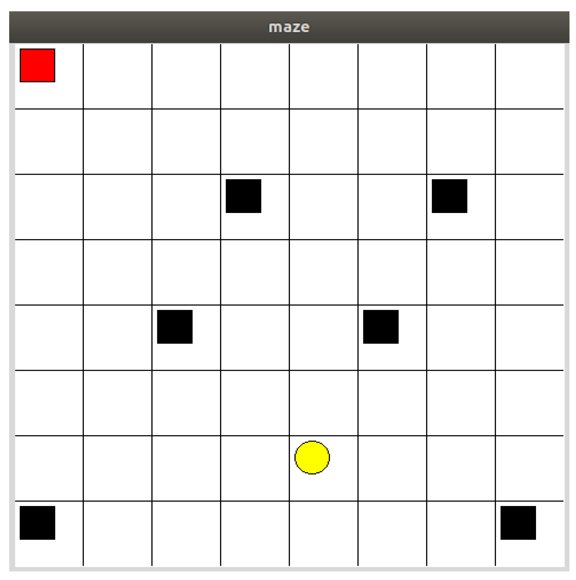
In this work, we use the Maze model to verify the effectiveness of the IPD3QN algorithm for USV path planning. The experimental environment is Python 3.6, Tensorflow 2.4, Ubuntu 18.0, Tkinter, and Maze model (as shown in Figure 1). The environment feature model is represented using the raster method, which divides the environment map into a number of equally sized rasters, with black rasters for obstacles, white rasters for free space, and yellow rasters for target space, each representing a state, so that the complex map environment is divided into feasible and infeasible spaces. The sea environment in which the USV is located is assumed to be a two-dimensional environment [26]. The two-dimensional space is discretized into a grid of 8 × 8 raster lengths. Then the specific element information of the environment is arranged according to the actual sea environment records. The area of the obstacle edge less than one grid area is set according to one grid, and finally, the grid serial number is recorded for the simulated set grid.

The experiment sets up four movements, namely up, down, left, and right, for the USV to explore according to the environmental state space. The environmental model and the moving process should be reasonably specified as follows. (1) To reduce the complexity of the experiment, the USV is regarded as a mass point. The movement of the USV can be treated as the process of pointing into a line, which ensures the implementation ability of the algorithm. (2) The effect on the ocean information factor is neglected. (3) Based on the physical point of view, the obstacles and the USV are mutual references during the navigation, so all obstacles such as reefs in the sea are processed in parallel.

In the experiments, we calculate the average reward every ten episodes for a total of 1000 episodes. The threshold of the termination episode is set to $\Delta =250$. In this case, the task automatically terminates if the USV cannot reach the target point after 250 episodes or encountering obstacles within 250 episodes. Moreover, the reward function is set as:

$$Reward=\left\{\begin{array}{ccc}\hfill 100,& & reachthetargetpoint\hfill \\ \hfill -10,& & reachtheobstaclepoint\hfill \\ \hfill 0,& & other\hfill \end{array}\right.$$

Similar to the Cartpole environment, we use $\mathcal{M}=70$ and $\mathcal{N}=50$ as the convergence condition in the Maze environment. Also, we use the same settings as the Cartpole environment for the six models, except that we set the number of neurons in the hidden layer as 20. The hyperparameter settings of the reinforcement learning algorithm are shown in

Table 3. Algorithm Hyperparameter Settings In Maze Environment.

Hyperparameter	Value	Remark
Minibatch	32	Participate in the training data set
Replay memory size	10,000	The capacity of the experience replay pool
Discount factor	0.9
Learning rate	0.0001	Adam gradient descent algorithm learning rate
$ϵ$	0.005	Update factor
$\alpha$	0.5	Control the degree of priority use
$\beta$	0.6	Importance sampling correction degree

. The dynamic $ϵ$-greedy Equation is as Equation (19).

$$\epsilon =\frac{{(t/1.8+25)}^3}{180}{e}^{-\sqrt{t/2+25}}$$

(19)

4.2. Result Analysis

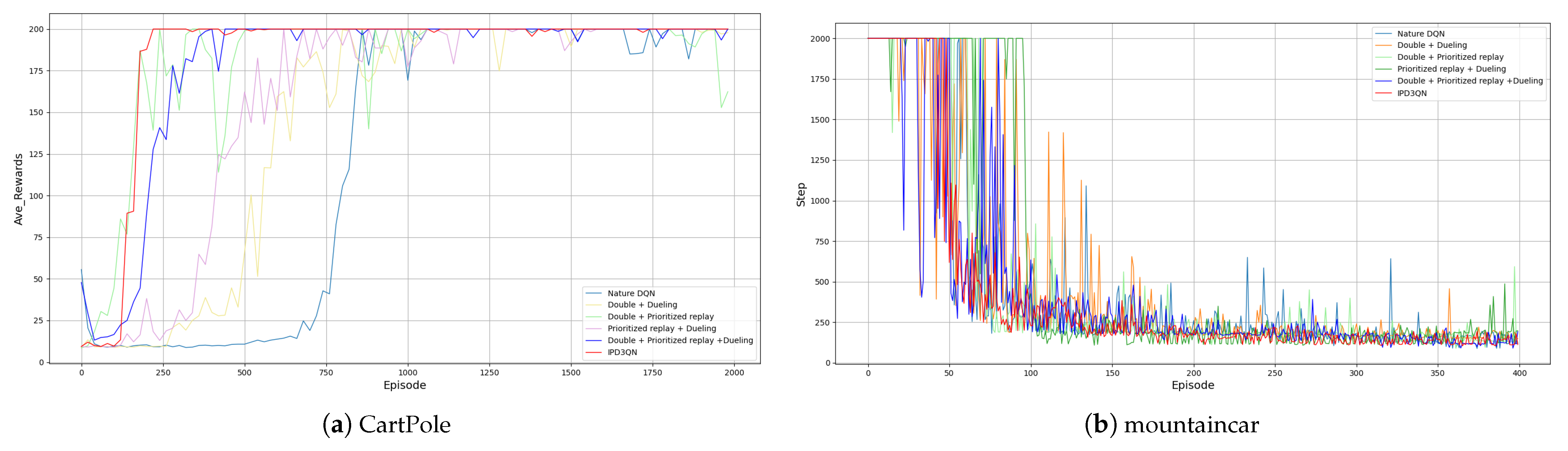
The six algorithms DQN, D3QN, PD2QN, PDQN, PD3QN, and IPD3QN, are compared in the Cartpole and MountainCar scenarios. The experimental results are shown in Figure 2,

Table 4. Comparison of Convergence Speed In Two Environments.

	Cartpole	Mountaincar
Nature DQN	900	187
Double + Dueling DQN	1040	242
Double + Prioritized Replay DQN	500	185
Prioritized Replay + Dueling DQN	1160	216
Double + Dueling +
Prioritized Replay DQN	440	184
IPD3QN	220	163

and

Table 5. Comparison of Convergence Stability In Two Environments.

	Cartpole	Mountaincar
Nature DQN	(197.75636, 5.82318)	(182.10329, 74.3346)
Double + Dueling DQN	(199.0625, 3.88483)	(174.60759, 38.2677)
Double + Prioritized Replay DQN	(197.14933, 9.86685)	(176.34419, 55.17239)
Prioritized Replay + Dueling DQN	(199.3667, 2.29406)	(168.19022, 52.08878)
Double + Dueling +
Prioritized Replay DQN	(199.52436, 1.63458)	(165.2222, 40.68757)
IPD3QN	(199.7827, 0.7394)	(152.37131, 34.27435)

. It can be concluded from the data in Table 4 that IPD3QN converges faster than the rest. It can be concluded from the data in Table 5 that the average reward of IPD3QN is greater than the other algorithms in the Cartpole environment. The standard deviation is reduced by 87.3%, 80.1%, 92.5%, 67.8%, 54.8% compared with DQN, D3QN, PD2QN, PDQN, PD3QN, respectively. In the Mountain Car environment, the convergence rate of IPD3QN is lower than the other algorithms, and the standard deviation is reduced by 53.9%, 10.4%, 37.9%, 34.2%, 15.8% compared with DQN, D3QN, PD2QN, PDQN, PD3QN, respectively. To conclude, the proposed IPD3QN algorithm has significantly improved the convergence speed and stability compared with other algorithms.

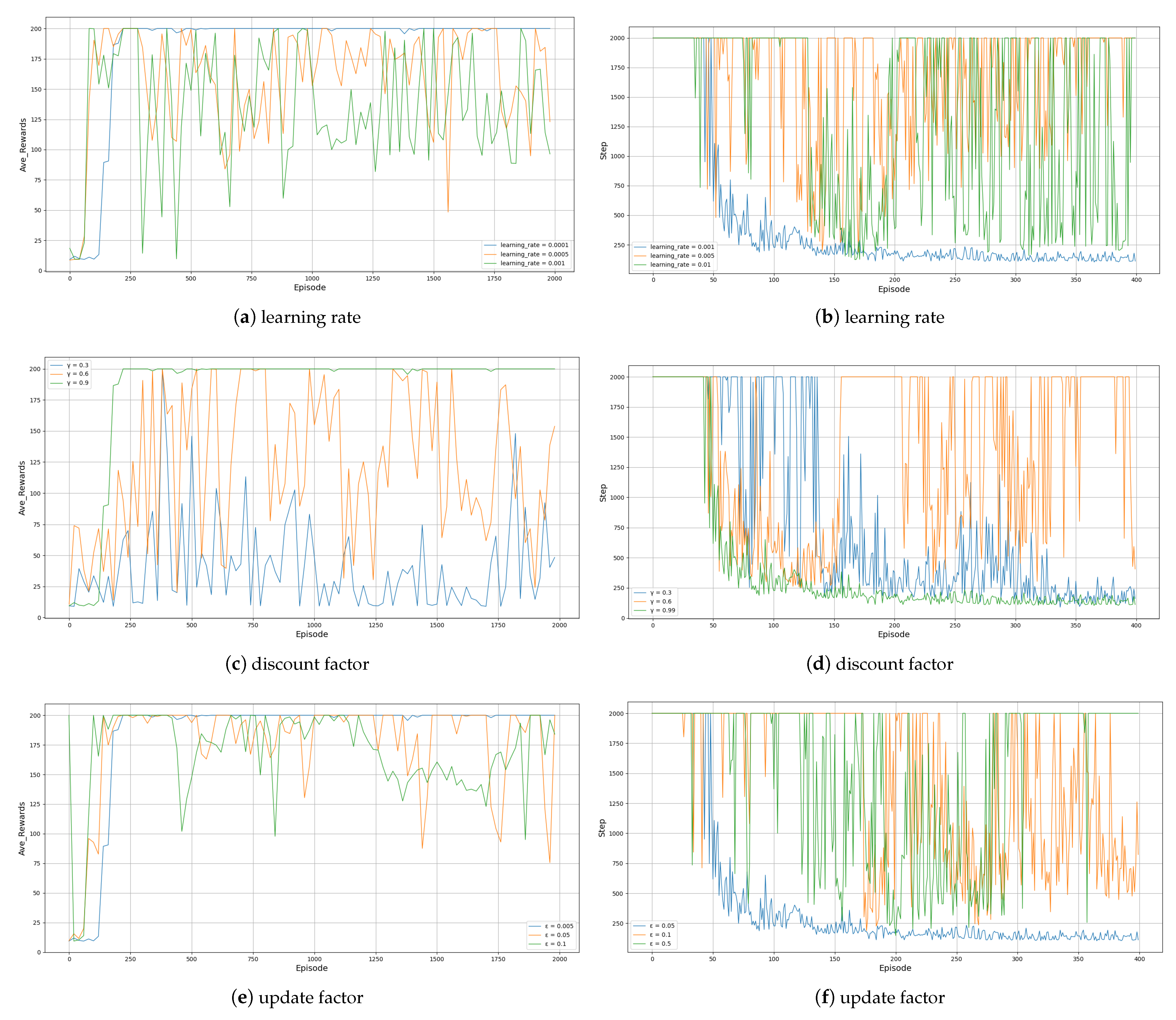
The effects of different learning rates on the convergence rate and convergence stability are given in Figure 3a,b. It can be seen that in the Cartpole and Mountain Car environments, the learning process is more stable when the learning rate is low. When the learning rate is large, although the learning can be accelerated in the early stage, it is persistently oscillating and challenging to converge in the later stage.

Figure 3c,d reflect the effect of the discount factor $\gamma$ on the convergence speed and convergence stability. It can be seen that when $\gamma$ is larger, the greater the influence of future returns on the current expected return value, the higher the proportion of future returns predicted in it when the intelligence calculates the expected return, which is beneficial to the learning environment and uses less training time. So $\gamma$ needs to be set large when the environment has a strong temporal correlation.

The effects of different interval update coefficients on the convergence speed and convergence stability are given in Figure 3e,f. It can be seen that in the Cartpole and Mountain Car environments, the learning process is more stable when the interval coefficient is small. When the interval coefficient is large, although it can be explored faster in the early stage, it is persistently oscillating and challenging to converge in the later stage.

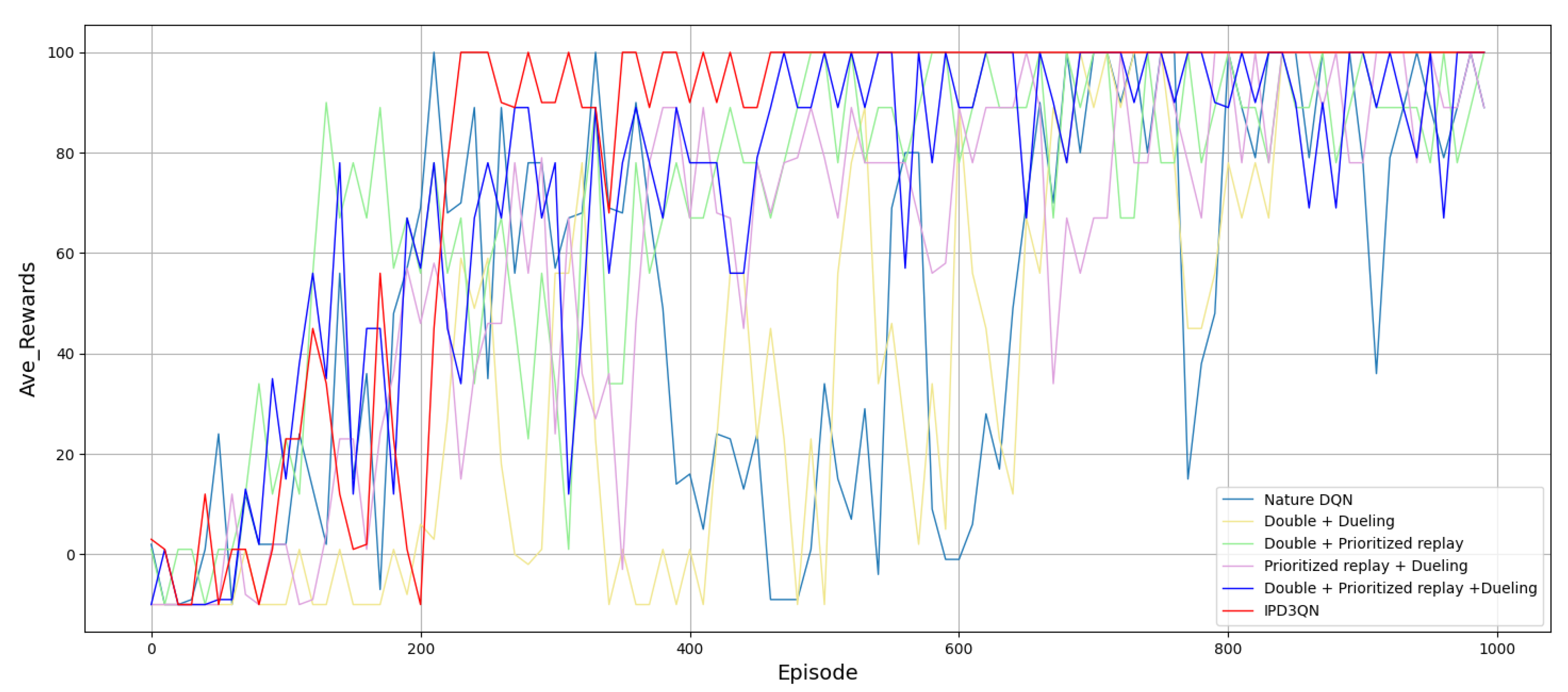
Through pre-verification in CartPole and mountaincar environments, experiments prove that IPD3QN can improve stability and convergence. Compare the six algorithms of DQN, D3QN, PD2QN, PDQN, PD3QN, and IPD3QN in the Maze scenario. The experimental results are shown in Figure 4,

Table 6. Comparison of Convergence Speed In Maze Environments.

	Maze
Nature DQN	650
Double + Dueling DQN	670
Double + Prioritized Replay DQN	470
Prioritized Replay + Dueling DQN	520
Double + Dueling +
Prioritized Replay DQN	450
IPD3QN	220

and

Table 7. Comparison of Convergence Stability In Maze Environments.

	Maze
Nature DQN	(84.4571, 37.3110)
Double + Dueling DQN	(89.6666, 32.1406)
Double + Prioritized Replay DQN	(89, 33.0312)
Prioritized Replay + Dueling DQN	(84, 38.7681)
Double + Dueling +
Prioritized Replay DQN	(92.0545, 28.0508)
IPD3QN	(97.8205, 15.0862)

. The data in Table 6 shows that IPD3QN converges faster than the rest; the data in Table 7 shows that in the maze environment, the average reward of IPD3QN is greater than Other algorithms, and the standard deviation compared with DQN, D3QN, PD2QN, PDQN, PD3QN reduced by 59.6%, 53.1%, 54.3%, 61.1%, 46.2%, performance is more stable.

To sum up, compared with other algorithms, the IPD3QN algorithm in this article has significantly improved convergence speed and convergence stability.

5. Conclusions and Future Work

This paper proposes an Improved Dueling Deep Double-Q Network Based on Prioritized Experience Replay (IPD3QN) to address the slow and unstable convergence of traditional Deep Q Network (DQN) algorithms in autonomous path planning of USV. First, we use the deep double Q-Network to decouple the selection and calculation of the target Q value action to eliminate overestimation. The prioritized experience replay method is adopted to extract experience samples from the experience replay unit, increase the utilization rate of actual samples, and accelerate the training speed of the neural network. Then, the neural network is optimized by introducing a dueling network structure. Finally, the soft update method is used to improve the stability of the algorithm, and the dynamic $ϵ$-greedy method is used to find the optimal strategy. The experiments are first conducted in the Open AI Gym test platform to pre-validate the algorithm for two classical control problems: the Cart pole and Mountain Car problems. The impact of algorithm hyperparameters on the model performance is analyzed in detail. The algorithm is then validated in the Maze environment. The comparative analysis of simulation experiments shows that IPD3QN has a significant improvement in learning performance regarding convergence speed and convergence stability compared with DQN, D3QN, PD2QN, PDQN, PD3QN. Also, USV can plan the optimal path according to the actual navigation environment with the IPD3QN algorithm. However, the IPD3QN algorithm proposed in this paper uses USV as a mass point and can only be simulated in discrete action scenarios. Constructing the USV’s motion model in the complex sea area and solving the problems of the convergence speed and convergence stability of the USV in the path planning under the complex continuous action scene are the focus of the next step of this paper.

References

1. Yuh, J.; Marani, G.; Blidberg, D.R. Applications of marine robotic vehicles. Intell. Serv. Robot. 2011, 4, 221–231. [Google Scholar] [CrossRef]
2. Bae, H.; Kim, G.; Kim, J.; Qian, D.; Lee, S. Multi-robot path planning method using reinforcement learning. Appl. Sci. 2019, 9, 3057. [Google Scholar] [CrossRef] [Green Version]
3. Qu, C.; Gai, W.; Zhong, M.; Zhang, J. A novel reinforcement learning based grey wolf optimizer algorithm for unmanned aerial vehicles (UAVs) path planning. Appl. Soft Comput. 2020, 89, 106099. [Google Scholar] [CrossRef]
4. Holen, M.; Saha, R.; Goodwin, M.; Omlin, C.W.; Sandsmark, K.E. Road detection for reinforcement learning based autonomous car. In Proceedings of the 2020 the 3rd International Conference on Information Science and System, Cambridge, UK, 19–22 March 2020; pp. 67–71. [Google Scholar]
5. Mnih, V.; Kavukcuoglu, K.; Silver, D.; Rusu, A.A.; Veness, J.; Bellemare, M.G.; Graves, A.; Riedmiller, M.; Fidjeland, A.K.; Ostrovski, G.; et al. Human-level control through deep reinforcement learning. Nature 2015, 518, 529–533. [Google Scholar] [CrossRef] [PubMed]
6. Xu, J.; Tian, Y.; Ma, P.; Rus, D.; Sueda, S.; Matusik, W. Prediction-guided multi-objective reinforcement learning for continuous robot control. In Proceedings of the International Conference on Machine Learning, PMLR, New York, NY, USA, 13–18 July 2020; pp. 10607–10616. [Google Scholar]
7. Glimcher, P. Understanding dopamine and reinforcement learning: The dopamine reward prediction error hypothesis. Proc. Natl. Acad. Sci. USA 2011, 108, 15647–15654. [Google Scholar] [CrossRef] [PubMed] [Green Version]
8. Watkins, C.J.; Dayan, P. Q-learning. Mach. Learn. 1992, 8, 279–292. [Google Scholar] [CrossRef]
9. Kober, J.; Bagnell, J.A.; Peters, J. Reinforcement learning in robotics: A survey. Int. J. Robot. Res. 2013, 32, 1238–1274. [Google Scholar] [CrossRef] [Green Version]
10. Chen, C.; Chen, X.Q.; Ma, F.; Zeng, X.J.; Wang, J. A knowledge-free path planning approach for smart ships based on reinforcement learning. Ocean Eng. 2019, 189, 106299. [Google Scholar] [CrossRef]
11. Precup, R.E.; Preitl, S.; Petriu, E.; Bojan-Dragos, C.A.; Szedlak-Stinean, A.I.; Roman, R.C.; Hedrea, E.L. Model-based fuzzy control results for networked control systems. Rep. Mech. Eng. 2020, 1, 10–25. [Google Scholar] [CrossRef]
12. Messinis, S.; Vosniakos, G.C. An agent-based flexible manufacturing system controller with Petri-net enabled algebraic deadlock avoidance. Rep. Mech. Eng. 2020, 1, 77–92. [Google Scholar] [CrossRef]
13. Sutton, R.S.; McAllester, D.A.; Singh, S.P.; Mansour, Y. Policy gradient methods for reinforcement learning with function approximation. NIPs Citeseer 1999, 99, 1057–1063. [Google Scholar]
14. Sutton, R.S. Learning to predict by the methods of temporal differences. Mach. Learn. 1988, 3, 9–44. [Google Scholar] [CrossRef]
15. Thrun, S.; Schwartz, A. Issues in using function approximation for reinforcement learning. In Proceedings of the Fourth Connectionist Models Summer School, Hillsdale, NJ, USA, 13 December 1993; pp. 255–263. [Google Scholar]
16. Van Hasselt, H.; Guez, A.; Silver, D. Deep reinforcement learning with double q-learning. In Proceedings of the AAAI Conference on Artificial Intelligence, Phoenix, AZ, USA, 12–17 February 2016; pp. 2094–2100. [Google Scholar]
17. Wang, Z.; Schaul, T.; Hessel, M.; Hasselt, H.; Lanctot, M.; Freitas, N. Dueling network architectures for deep reinforcement learning. In Proceedings of the International Conference on Machine Learning, PMLR, New York, NY, USA, 19–24 June 2016; pp. 1995–2003. [Google Scholar]
18. Schaul, T.; Quan, J.; Antonoglou, I.; Silver, D. Prioritized experience replay. arXiv 2015, arXiv:1511.05952. [Google Scholar]
19. Hou, Y.; Liu, L.; Wei, Q.; Xu, X.; Chen, C. A novel DDPG method with prioritized experience replay. In Proceedings of the 2017 IEEE International Conference on Systems, Man, and Cybernetics (SMC), Banff, AB, Canada, 5–8 October 2017; pp. 316–321. [Google Scholar]
20. OpenAi-Gym. CartPole-v0. Available online: https://github.com/openai/gym/wiki/CartPole-v0. (accessed on 19 August 2021).
21. Xu, Z. Research on deep reinforcement learning algorithm based on dynamic fusion target. Comput. Eng. Appl. 2019, 55, 162–166. [Google Scholar]
22. Zamora, I.; Lopez, N.G.; Vilches, V.M.; Cordero, A.H. Extending the openai gym for robotics: A toolkit for reinforcement learning using ros and gazebo. arXiv 2016, arXiv:1608.05742. [Google Scholar]
23. Malla, N.; Ni, Z. A new history experience replay design for model-free adaptive dynamic programming. Neurocomputing 2017, 266, 141–149. [Google Scholar] [CrossRef]
24. Barto, A.G.; Sutton, R.S.; Anderson, C.W. Neuronlike adaptive elements that can solve difficult learning control problems. IEEE Trans. Syst. Man Cybern. 1983, SMC-13, 834–846. [Google Scholar] [CrossRef]
25. Cannon, R.H. Dynamics of Physical Systems; Courier Corporation: North Chelmsford, MA, USA, 2003. [Google Scholar]
26. Etemad, M.; Zare, N.; Sarvmaili, M.; Soares, A.; Machado, B.B.; Matwin, S. Using deep reinforcement learning methods for autonomous vessels in 2d environments. arXiv 2020, arXiv:2003.10249. [Google Scholar]
Figure 1. Maze Environmental Diagram.
Jmse 09 01267 g001
Figure 2. Comparison Of Different Algorithms In Two Environments.
Jmse 09 01267 g002
Figure 3. In Two Environments, The Impact Of Different Parameters On IPD3QN.
Jmse 09 01267 g003
Figure 4. Comparison Of Different Algorithms In Maze Environments.
Jmse 09 01267 g004