Estimating the Annual Exceedance Probability of Water Levels and Wave Heights from High Resolution Coupled Wave-Circulation Models in Long Island Sound

Abstract

Accurately estimating the probability of storm surge occurrences is necessary for flood risk assessments. This research models Long Island Sound using a coupled coastal circulation and wave model (FVCOM-SWAVE) to hindcast the 44 highest storms between 1950–2018 and fitted Poisson-GPD distributions to modelled water levels and wave heights. Floodwater elevations and significant wave heights for 10% (1/10), 3% (1/30), 2% (1/50), and 1% (1/100) annual exceedance probabilities are provided for all Connecticut coastal towns. The results show that both water levels and their corresponding return intervals are higher along the western coast of Connecticut than the eastern coast, whereas significant wave heights increase eastward. Comparing our model results with those from the North Atlantic Coast Comprehensive Study (NACCS) shows that the mean NACCS results are higher for water levels and lower for significant wave heights for longer return periods. Likewise, the Federal Emergency Management Agency (FEMA) results in large errors compared to our results in both eastern and western coastal Connecticut regions. In addition to evaluating historical risks, we also added a sea-level height offset of 0.5 m for 2050 estimates in order to examine the effect of rising sea-levels on the analysis. We find that sea-level rise reduces the return period of a 10-year storm to two years. We advise periodically updating this work as improved sea-level rise projections become available.

1. Introduction

Storm flooding is a destructive event that damages infrastructure, especially in coastal areas with low elevations. The state of Connecticut suffered around $360 million in damages after Hurricane Sandy alone [1]. Damages caused by increased water levels from historic storm surges and waves in low-lying areas can be used in order to estimate the potential for future damage from similar events. In addition, because rising sea-levels increase the frequency of storm-induced high water levels, an understanding of the effect of sea-level rise on risk trends is necessary for evaluating future storm and hurricane inundation risk [2,3,4,5]. O’Donnell [6] emphasized that storm-related flood risks would increase as the sea-level rose. Therefore, storm-induced flooding risk assessments should include the effect of sea-level rise, and we use an upper bound of 50 cm sea-level rise by 2050 for Connecticut [6].

The Federal Emergency Management Agency (FEMA) and the North Atlantic Coast Comprehensive Study (NACCS) [7] evaluated the 1% annual chance of flood events in Long Island Sound (LIS). FEMA’s approach for estimating floodplain maps included a regional statistical approach applied to the New London, New Haven, and Bridgeport tide gauge stations to compute probability distributions of the data at the gauges. FEMA computed deep-water wave characteristics using empirical wind-wave growth equations that were applied to Tweed New Haven Regional Airport historical data and then calculated along an inland transect to compute the overland wave propagation using the model WHAFIS [8]. One of the drawbacks of this approach is that storm surges are interpolated over only three stations, and calculated incident wave heights do not consider refraction, diffraction, or bottom dissipation effects.

The NACCS study used observations from extratropical storms using the method described by [9], which was then applied to synthetic tropical storms using the LIS model and analyzed using an optimum sampling of the joint probability method [10,11,12]. The deep-water wave boundary was obtained in 0.083-degree resolution and 0.25-degree wind resolution by solving the action-balance equation in the WAM model [13], which produced nearshore steady-state wave model results using STWAVE [14] and simulated surge and circulation results using ADCIRC [15]. Even though the NACCS study was more sophisticated than the FEMA study, the storm surge model was of coarse resolution to simulate total water levels in the coastal floodplains of the Connecticut coasts [16,17]. Like FEMA, NACCS did not include the effect of sea-level rise on return intervals, which is essential for future risk planning at local scales [18].

Understanding the probability of a flood event influences coastal policy and management. A down-scaled comprehensive understanding of total wave elevations can aid in assessing the risks, consequences of design costs, and environmental impacts of coastal plans [19]. Furthermore, the return period analysis in LIS should be updated at a higher resolution. This study aims to provide storm surge and wave height probabilities to aid the engineers and planners in developing cost-effective design criteria for resiliency projects.

We calibrated and applied a coupled coastal circulation and wave model system to estimate the frequency of occurrences of extreme storms using hindcasts of historical storms with different return periods for each town along the LIS coast in Connecticut. Our work demonstrates a method and technique for enclosed sounds where circulation and wave modeling are challenging due to sparse data availability and unique geomorphologies. We also examined extreme events under both present and future sea-level conditions in order to understand the effect of sea-level rise on the generated wave characteristics.

Section 2 presents the study area, historical storm data, and data collected in Connecticut to build the circulation and wave model. Section 3 describes the wave and circulation models and methodology to obtain statistically independent storm events, the peak-over-threshold method, and error analysis. Section 4 presents our results by town and compares these with previous studies. Finally, Section 5 discusses the results and presents our conclusions.

2. Background

2.1. Study Area and In-Situ Data

LIS is a semi-enclosed estuary that is connected to the Hudson River in the west through East River strait and the Mid Atlantic Bight through Block Island Sound in the east (Figure 1). The primary freshwater source for LIS is the Connecticut River, which provides 75% of the total discharge [20]. The unique geomorphology of LIS was created by the latest glacial period and is formed mostly of marshlands and beach ridges along the 1000-km Connecticut shoreline. The barotropic pressure gradient force generated from wind stress is the main source for subtidal circulation, sea-level fluctuations, and vertical mixing [20]. Extratropical storms called Nor’easters are the dominant storm source and generate large sea level anomalies in the western Sound due to the sea-surface height setup on the adjacent continental shelf [21]. The shelf morphology causes different return periods for similar water level anomalies in the western and eastern LIS. M${}_2$ (lunar semidiurnal) tides are dominant in LIS and have a mean range of 2.2 m [22]. Tidal height amplitudes increase in the western end. Tidal gauge and buoy locations are provided in

Table 1. The locations of the gauge and buoys from [23,24].

Station Name	Agency	Station Number	Latitude (${}^{\circ }$ N)	Longitude (${}^{\circ }$ W)	Record Starting Year
Kings Point	NOAA	8516945	40.81	73.765	1998
Bridgeport	NOAA	8467150	41.173	73.182	1970
New Haven	NOAA	8465705	41.283	72.908	1999
New London	NOAA	8461490	41.355	72.087	1938
Montauk	NOAA	8510560	41.048	71.765	1947
Execution Rocks (EXRX)	UConn	44022	40.956	73.580	2004
Western LIS (WLIS)	UConn	44040	40.956	73.580	2004
Central LIS (CLIS)	UConn	44039	41.138	72.655	2004
Ledge Light	UConn	LDLC3	41.306	72.077	2004

and Figure 1.

2.2. Wind Data

Wind data were taken from hourly records of 13 airports within or adjacent to the study area (Figure 1). The wind records were obtained from the local climatological dataset of the National Climate Data Center (NCDC), NOAA [25]. Generally, the airport records cover the entire study period (1950–2018). However, airports with missing data during certain extreme events were excluded to avoid biases due to correlations between extreme events and damaged instrumentation.

The airport winds were first bi-linearly interpolated to a 2D structured grid with a horizontal resolution of 0.02-degree longitude/latitude. Then, buoy observed winds [24,26] were used to calibrate the airport winds to represent over-water winds since the land-based measurements underestimated the winds over water. Four buoy stations (44022/EXRX, 44040/WLIS, 44039/CLIS, and LDLC3) in the LIS were used, covering a period from 2004 to 2019. Only easterly winds higher than 10 m s${}^{-1}$ were compared, as high water level events occur under strong easterly winds. The overall comparison shows that, on average, the buoy observations are approximately 1.7 times that of the airport interpolations in the eastern and central Sound (at CLIS and LDLC3) and 1.5 times in the western Sound (WLIS and EXRX). Based on this relationship, the interpolated wind field was adjusted accordingly, following:

$${\mathbf{U}}_{\mathbf{X}}^{\prime }=F_{\mathbf{X}}{\mathbf{U}}_{\mathbf{X}},$$

(1)

where $\mathbf{X}$ is the two-dimensional geographical location, ${\mathbf{U}}_{\mathbf{X}}=[u_{\mathbf{X}},v_{\mathbf{X}}]$ is the wind field bi-linearly interpolated from airport observations, ${\mathbf{U}}_{\mathbf{X}}^{\prime }$ is the adjusted wind field, and $F_{\mathbf{X}}$ is an adjustment coefficient field defined as:

$$F_{\mathbf{X}}=\left\{\begin{array}{cc}1.7,\hfill & \mathbf{X}={\mathbf{X}}_{\mathrm{CLIS}},{\mathbf{X}}_{\mathrm{LDLC}3}\hfill \\ 1.5,\hfill & \mathbf{X}={\mathbf{X}}_{\mathrm{EXRX}},{\mathbf{X}}_{\mathrm{WLIS}}\hfill \\ 1,\hfill & \mathbf{X}={\mathbf{X}}_{\mathrm{airports}}\hfill \\ \mathrm{bi}-\mathrm{linearly}\mathrm{interpolated},\hfill & \mathrm{elsewhere}.\hfill \end{array}\right..$$

(2)

A total of 44 storm events, including severe historical hurricanes and Nor’easters, were selected based on high water level records from NOAA tidal stations in Bridgeport and New London, Connecticut (

Table 2. List of severe historical storms in Long Island Sound.

No.	Date	Storm Type and Name	No.	Date	Storm Type and Name
1	25 Nov 1950	Extratropical	23	4 Feb 1995	Extratropical
2	7 Nov 1953	Extratropical	24	20 Mar 1996	Extratropical
3	31 Aug 1954	Tropical (Hurricane Carol)	25	19 Oct 1996	Extratropical
4	16 Feb 1958	Extratropical	26	21 Aug 1997	Extratropical
5	19 Feb 1960	Extratropical	27	6 Nov 2002	Extratropical
6	12 Sep 1960	Tropical (Hurricane Donna)	28	16 Dec 2005	Extratropical
7	12 Nov 1968	Extratropical	29	28 Oct 2006	Extratropical
8	5 Apr 1973	Extratropical	30	16 Apr 2007	Extratropical
9	10 Jan 1977	Extratropical	31	12 Dec 2008	Extratropical
10	9 Jan 1978	Extratropical	32	14 Mar 2010	Extratropical
11	7 Feb 1978	Extratropical	33	27 Dec 2010	Extratropical
12	25 Dec 1978	Extratropical	34	17 Apr 2011	Extratropical
13	25 Oct 1980	Extratropical	35	28 Aug 2011	Tropical (Hurricane Irene)
14	29 Mar 1984	Extratropical	36	12 Jan 2012	Extratropical
15	27 Sep 1985	Tropical (Hurricane Gloria)	37	5 Jun 2012	Extratropical
16	23 Jan 1987	Extratropical	38	30 Oct 2012	Tropical (Hurricane Sandy)
17	22 Oct 1988	Extratropical	39	27 Dec 2012	Extratropical
18	19 Aug 1991	Tropical (Hurricane Bob)	40	14 Mar 2017	Extratropical
19	31 Oct 1991	Extratropical	41	30 Oct 2017	Extratropical
20	11 Dec 1992	Extratropical	42	2 Mar 2018	Extratropical
21	13 Mar 1993	Extratropical	43	27 Oct 2018	Extratropical
22	24 Dec 1994	Extratropical	44	16 Nov 2018	Extratropical

). Simulated storm model output encompassed from 3 to 6 days.

3. Methodology

3.1. Circulation and Wave Model

The Finite Volume Community Ocean Model (FVCOM) [27,28] was used to hindcast historical storm events in LIS. FVCOM is an unstructured-grid, 3D primitive equation ocean circulation model. FVCOM was coupled to an adapted Simulating Wave Nearshore (SWAN) model [29]. The coupled FVCOM-SWAVE model incorporates the exchange of wave radiation stresses, as well as near-bottom and surface shear stresses [28,30].

The model grid used is described in O’Donnell et al. [31]. The model domain covers Long Island Sound, Block Island Sound, and the adjacent shelf south of Long Island (Figure 1). The horizontal resolution is 500 m along the coast and 5 km in open water. There are ten evenly distributed vertical $\sigma$ layers through the water column. Vertical eddy diffusivity was capped at 0.04 m${}^2$s${}^{-1}$ to have water level results that better match the observational data. Quadratic bottom friction is adopted with a spatial varying roughness length parameter $z_0$. Specifically, $z_0$ is set to 0.003 m, where depth ≤ 40 m and decreases towards zero as the depth increases [32]. The time step was set to 3 s for the external mode and 18 s for the internal mode.

Time series of surface water elevations along the open boundary were prescribed. The time series was first reconstructed using eight astronomical tidal constituents, including M${}_2$, N${}_2$, S${}_2$, O${}_1$, K${}_1$, K${}_2$, P${}_1$, and Q${}_1$, which are extracted from a northwest Atlantic regional FVCOM model [33]. Then, the reconstructed signals were subsequently adjusted by the difference between the NOAA water level observations at the Montauk, NY station and reconstructed tidal signals at Montauk (Figure 1). Since Montauk is close to the open boundary, such an adjustment corrects the open boundary elevation for subtidal and shelf water elevation variations.

Wave parameters used are summarized in

Table 3. Model parameters used for FVCOM-SWAVE.

Direction bins	24
Frequency bins	24
Minimum frequency (Hz)	0.05
Maximum frequency (Hz)	0.5
Wind input	Komen formulation
Cavaleri and Malanottee’s wave growth term	Activated, a = 0.0015
Quadruplet nonlinear interactions	Activated
Triad nonlinear interactions	Deactivated
White capping dissipation	Komen formulation
Bottom friction	JONSWAP

. Wave open boundary conditions for events after 1979 are obtained from NOAA Northwest Atlantic WAVEWATCH III 30-year Hindcast [34,35] (available from https://polar.ncep.noaa.gov/waves/hindcasts/), including significant wave heights, wave directions, and peak periods. Events before 1979 have no wave input at the open boundary due to data unavailability.

3.2. Extreme Value Analysis

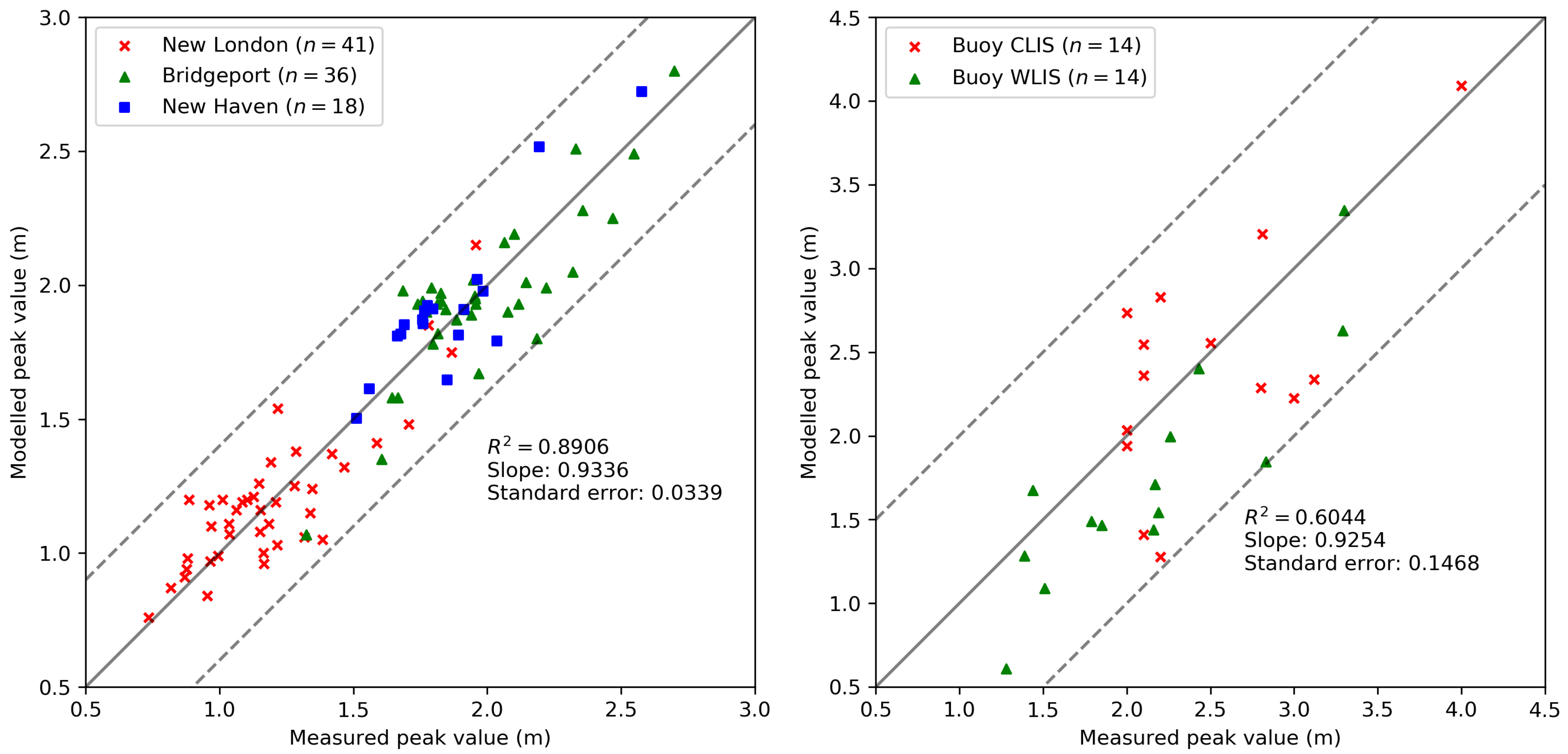
The general procedures we employed are divided into four steps: (i) analyzing water level and wave heights obtained from the circulation and wave model to obtain statistically independent storm data; (ii) calculating the empirical probability distribution of extreme water levels; (iii) fitting the combined Poisson-Generalized Pareto Distributions (GPD) to the model distributions; and (iv) calculating return levels using the best-fit shape and scale parameters within the desired confidence level.

The model-computed peak storm wave heights and water levels were ranked in descending order from the highest to lowest to identify statistically independent storm events. An empirical probability distribution was estimated from [36]

$$Q\left(H\right)=\frac{m}{N+1},$$

(3)

where Q is the probability of exceedance, m is the rank of the peak storm wave height and water level, and N is the total number of observed peak storm wave heights and water levels.

The Generalized Pareto Distribution (GPD) is an asymptotic distribution often used to estimate extreme values above a specific threshold, and the combination of a Poisson distribution and GPD in a peak-over-threshold (POT) framework results in a Generalized Extreme Value (GEV) distribution [37]. This methodology produces distributions of annual maxima, which (in our case) are neither directly observed nor directly modeled. The Poission-GPD method produces the best fit among the generalized extreme value distribution types by minimizing the differences in the empirical distributions between the buoy/gauge observations and the modeled water level results. We applied the Poission-GPD method to the modeled peak water level and significant wave heights from 44 modeled extreme storm events using the MATLAB package WAFO [38]. The individual peak values were obtained from defined storm events with a duration longer than an hour.

For each location, the GPD was fitted to modeled extreme values with a cumulative distribution function

$$F(z;u,\sigma ,\xi )=1-{\left(1+\xi \frac{z-u}{\sigma }\right)}^{-1/\xi },\xi \ne 0,z>u,$$

(4)

where u is the threshold which was determined using the dispersion index method implemented in the WAFO package, $\sigma$ is the scale parameter, and $\xi$ is the shape parameter. The maximum of a Poisson distributed number of independent GPD variables has a GEV distribution [37,39,40]. Based on the assumption that the annual threshold exceedances u is Poisson distributed, the cumulative distribution function for the annual maximum Poisson-GPD and GEV relationship and parameter transformation [37,39,40] is:

$$G\left(z\right)=exp(-\lambda [1-F\left(z\right)])=exp\left(-\lambda {\left(1-\xi {\displaystyle \frac{z-u}{\sigma }}\right)}^{-1/\xi }\right).$$

(5)

where $\lambda$ is the Poisson mean parameter that is estimated by dividing the total number of exceedances of threshold, u, by the total number of years. Rearranging Equation (5), we get the traditional form of the GEV cumulative distribution function:

$$G(z;\mu ,\psi ,\xi )=exp\left(-{(1+\xi \frac{z-\mu }{\psi })}^{-1/\xi }\right),\xi \ne 0,z>\mu$$

(6)

where the scale parameter $\psi ={\displaystyle \frac{\sigma }{{\lambda }^{\xi }}}$, and the location parameter $\mu =u+\psi \left({\displaystyle \frac{{\lambda }^{\xi }-1}{\xi }}\right)$.

The return period is defined as the recurrence interval of a specific storm event water level or wave height (X) that is equal to or exceeds the average of successive events (x) within T years. The exceedance probability is Q, and the probability of occurrence $Q(X>x)$ in a given year is $Q=1/T$. Return periods were determined using the following relationship between the GEV return level $s_T$ and return period T:

$$s_T=\mu +{\displaystyle \frac{\psi }{\xi }}\left(1-(-log{\left(1-\frac{1}{T})\right)}^{\xi }\right).$$

(7)

Return years of the empirical data points Y were determined using the Weibull plotting position [36,41]

$$Y=\frac{N+1}{m}.$$

(8)

3.3. Error Analysis

The goodness of fit between the computed and observed peak water levels and wave heights were evaluated based on the absolute error, the root-mean-square error (RMSE), the correlation of determination (R${}^2$), the scatter index, the standard error, the HH index [42], and the Willmott score [43]. The fits were further compared by plotting computed and observed values against each other:

$$HH=\sqrt{\frac{\sum {\left(x_m-x_o\right)}^2}{\sum x_m{x}_o}},$$

(9)

$$W_s=1-\frac{\sum \left(x_m-x_o\right)}{\sum {\left(\left|x_m-{\overline{x}}_o\right|+\left|x_o-{\overline{x}}_o\right|\right)}^2},$$

(10)

where $x_m$ and $x_o$ are modeled and observed results, respectively. The HH index captures bias and scatter component. ${\overline{x}}_o$ is an average of the observed results. The Willmott score, $W_s$, captures the constant and proportional offset errors and indicates close agreement between model and observations when it is close to one. When it is zero, it indicates no agreement.

4. Results and Discussion

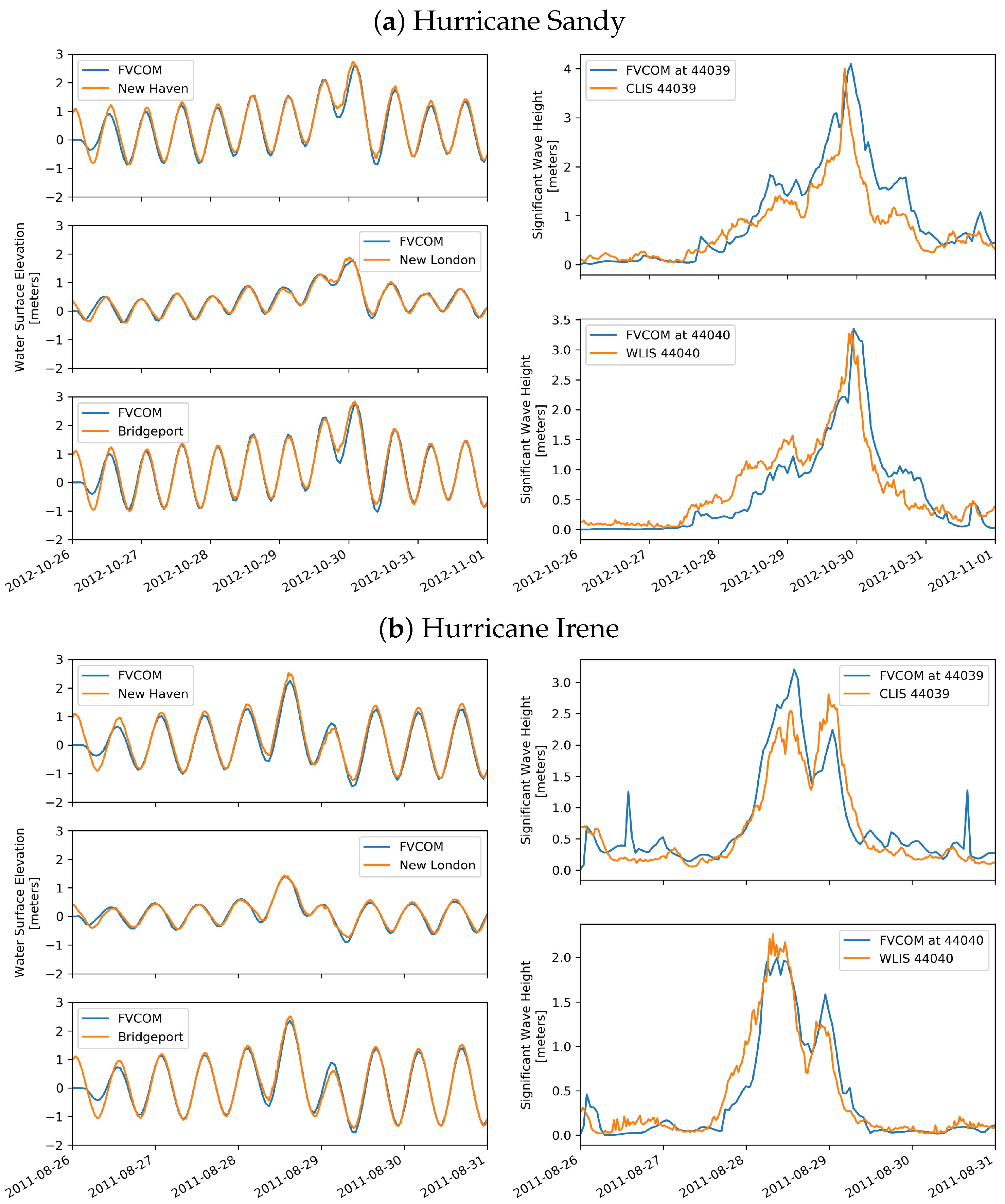
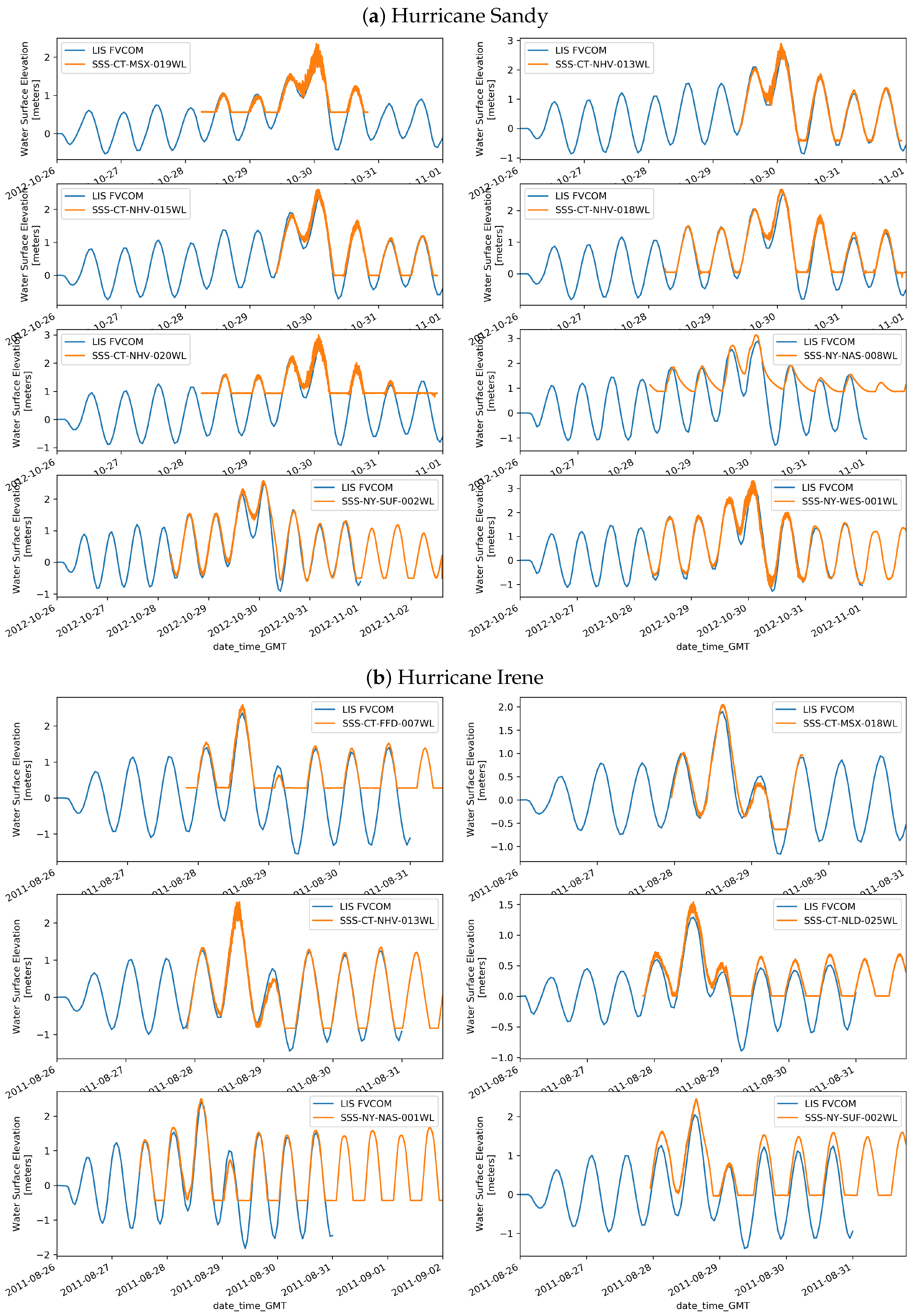
4.1. Validation of the Model

Modeled results from FVCOM-SWAVE were compared to observations from Kings Point, Bridgeport, New Haven, New London, and Montauk tide gauges for water levels associated with Hurricanes Irene and Sandy (Figure 2). Surface water elevations from the model aligns well with the tide gauge data for these events. Significant wave height comparisons between the model and observations at the buoy locations demonstrate good agreement at NDBC buoys 44025 and 44097 (not shown). The model also captured the peak storm significant wave height at the CLIS buoy location. The model-data agreement at the WLIS buoy at the peak of the event was low, possibly due to buoy measurement errors during the hurricane. The model results were also compared with USGS storm surge sensors (Figure 3). The reason for some sensors not matching with the model results during the downward zero-crossing (e.g., horizontal lines) was that they were on dry land at the time.

In addition to the time series comparison, the differences between the modeled and observed data were quantified using mean error, RMSE, R${}^2$, scatter index, standard error, HH index, and Willmot score for New London, New Haven and Bridgeport tide locations (

Table 4. Error metrics of the modeled and observed water levels.

Station Name	Absolute Error	RMSE	R${}^2$	Scatter Index	Standard Error	HH Index	Willmott Score
Bridgeport	0.133	0.165	0.713	0.0826	0.086	0.083	0.915
New Haven	0.146	0.146	0.777	0.0685	0.101	0.077	0.919
New London	0.123	0.150	0.721	0.1225	0.088	0.123	0.920
Total	0.127	0.155	0.891	0.0920	0.034	0.092	0.971

and Figure 4). Comparisons between the modeled and observed peak water elevations show good agreement. Although the error statistics for the individual locations were all close to each other, New Haven showed the closest fit and the least bias and scatter. The sample size at each of the stations may have contributed to these results. Overall, good fits were observed at all tide-gauges. The most substantial errors occurred at locations where peak levels were affected by water flow restrictions caused by local bathymetry. As the event duration increased, model skill at predicting water levels over the period decreased.

The empirical return level distributions were created using the Weibull plotting of the exceedance probability. For all tide locations, the empirical return level distribution of the FVCOM-generated peak water levels closely represented the observed water levels (Figure 5). The return level fitted to New London and Bridgeport demonstrated a similar water level series. The significant wave height distributions at the CLIS and WLIS buoys were slightly different with lower values at the WLIS location. Despite generating water levels that followed the observed gauge results, the model was unable to capture the exact shape of the significant wave height evolution. This issue was expected due to a lack of available wave data (less than 20 years) compared to water level data (over 60 years). Despite the limited observational wave data, the model represented peak significant wave heights well enough to develop exceedance probabilities.

4.2. Selection of GPD Threshold

Although the modeled data represent the historical conditions well, due to the upper tail uncertainty and the irregularity, fitted probability distributions were used to smooth out the historical data sample and use it for future return period projections. A user-defined threshold was required to represent the storms and hurricanes using GPD. For each of the model point locations corresponding to the coastal towns, we determined this threshold using the dispersion index method implemented in the WAFO package, which measures the homogeneity of data and determines a threshold such that the number of exceedances is consistent with a Poisson process with a dispersion index close to 1 [44]. It is fitted to top-ranked storms because it represents the tail end of the distribution that is above the threshold. For instance, using FVCOM water level outputs at Bridgeport, mean excess, modified scale, and shape tests showed that the model results presented high skewness above the threshold 1.82 m, which indicates the relative magnitude of deviations above the mean. The same procedure was applied to other locations. Therefore, even though the number of surge parameters was increased for estimating better return periods, we restricted the analysis to use the 44 top-ranked storm events through the threshold selection.

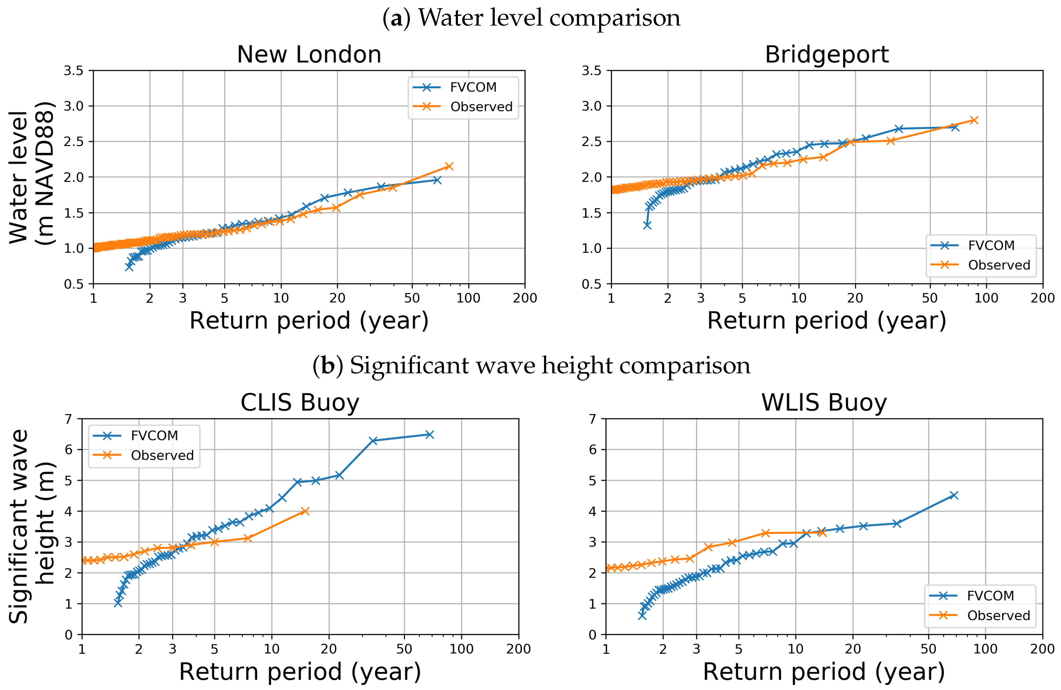
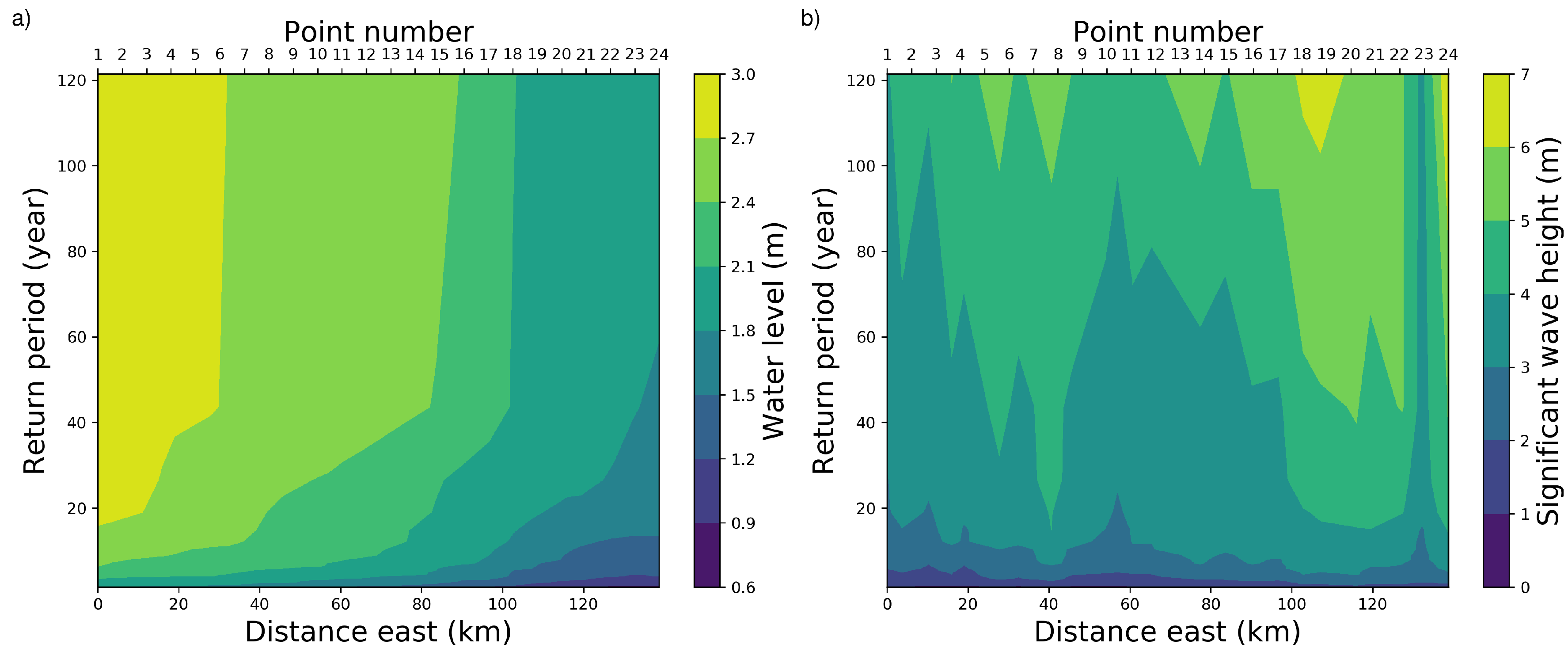
4.3. Annual Exceedance Probability Distributions

The return periods of water level exceedances varied from the west to the east (Figure 6). The highest water levels were in western LIS (near New York) and decreased eastward. This is likely contributed to by the water run-up in the Sound in response to wind forcing. The significant wave height increased around Bridgeport and east of New London.

The return period plots of water levels (Figure 7) and significant wave heights (Figure 8) for each town show the model results (dark blue dots), the Poisson-GPD fit (orange line), the mean of NACCS results [45] (light blue line, 95% confidence bound included). The Poisson-GPD fit was calculated using the best fit distribution of the model results. The return period and the corresponding water and wave height levels are listed in

Table 5. Corresponding water level (h) and significant wave height (Hs) for return periods.

Return Period	Bridgeport		New Haven		New London
Year	h (m)	Hs (m)	h (m)	Hs (m)	h (m)	Hs (m)
10	2.32	2.83	2.16	2.44	1.44	3.43
30	2.58	3.68	2.39	2.24	1.73	4.26
50	2.68	4.03	2.47	3.57	1.86	4.56
100	2.78	4.48	2.55	3.98	2.03	4.91

and the Supplementary Material. Floodwater elevations and significant wave heights for specific events such as 10% (1/10), 3% (1/30), 2% (1/50), 1% (1/100) annual exceedance probability were determined (refer to: Table 5, Appendix A and Appendix B and the Supplementary Materials).

4.4. Wind Accuracy and Sensitivity

For the spatial and temporal scales of this study, the airport wind records have better horizontal resolution and temporal coverage than hindcast winds from numerical simulations in the LIS region. For instance, the NCEP reanalysis [46] covers the whole study period but lacks spatial resolution, while regional weather models, such as WRF, have no qualified initial fields to support the simulation before 1979 (e.g., NARR, [47]). Our preliminary tests also showed that not even a 3-km resolution WRF model could capture the spatial asymmetry of wind speed observed from airport winds during Hurricane Sandy. Additionally, the WRF modeled hurricanes for events during the 1980s and 1990s are not as accurate as of the 2000s and later. This may be caused by less observational data assimilation into the NARR during the earlier decades. Due to relatively small spacing between airports around LIS, FVCOM performance is better when forced with the interpolated airport winds than with other hindcast wind products.

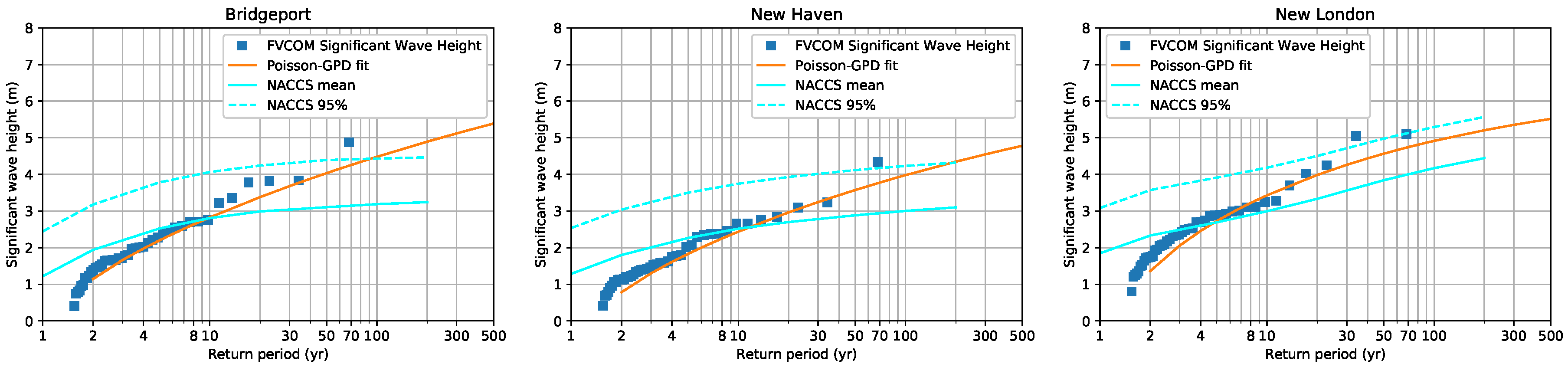
4.5. The Model Results Compared with NACCS and FEMA

The results presented here summarize the GPD analysis results with return interval estimates for storm surges and waves. At 10% annual exceedance, modeled water levels were all over 2.5 m. The water levels were highest in the west and gradually decreased alongshore eastward by 1 m. These model results are within the 95% confidence interval of the mean NACCS model results.

In general, the NACCS results show higher water levels compared to this study. However, the differences are somewhat reduced in the central Sound (between Fairfield and Waterford). A comparison with the FEMA results also shows that the differences are small in the central Sound, but, overall, water level in FEMA tends to be lower (Figure 9). In the eastern Sound, it is possible that both NACCS and FEMA either overestimate or underestimate the remote impacts of water level from the continental shelf [48,49], while, in the western Sound, the long fetch allows strong local wind to build up the water level [50]. Our comparisons indicate that both NACCS and FEMA may lack the ability to account for such processes.

The modeled significant wave heights show higher uncertainties after the 10% annual exceedance limit. At a 10% annual exceedance, our significant wave height estimates are over 2 m in the west and gradually increase alongshore eastward to over 3.5 m. Significant wave height from NACCS is overestimated below a 20% annual exceedance comparing to our results, but our results are still within the NACCS 95% confidence limits (Appendix B). At a 10% annual exceedance level, the NACCS results are higher in the central Sound (between Fairfield and Waterford shores). At longer return periods, however, the NACCS results for the significant wave height appear to be lower (Appendix B).

The model reproduces peak water level events well compared to the observations. An increase in both the model and wind field spatial resolution could increase the agreement of water level in coastal areas. The water level and significant wave height return periods provided in this study aim to assist planners and engineers in designing coastal protection in a limited near future time. Even assuming a steady-state flood risk environment, confidence intervals of the annual exceedance limits become very broad for longer return periods because the most extreme events are also the most uncommon and lacking observations. In addition, considering the non-static attributes of the environment, the model estimates for longer return periods are likely to be even less accurate than they would in a static environment. The modeled results are expected to be more accurate for the next ten years than the next 100 years. Hence, we recommend repeating this study every 10 years to take into account both the sea level rising and possible changes in storm frequency and intensity.

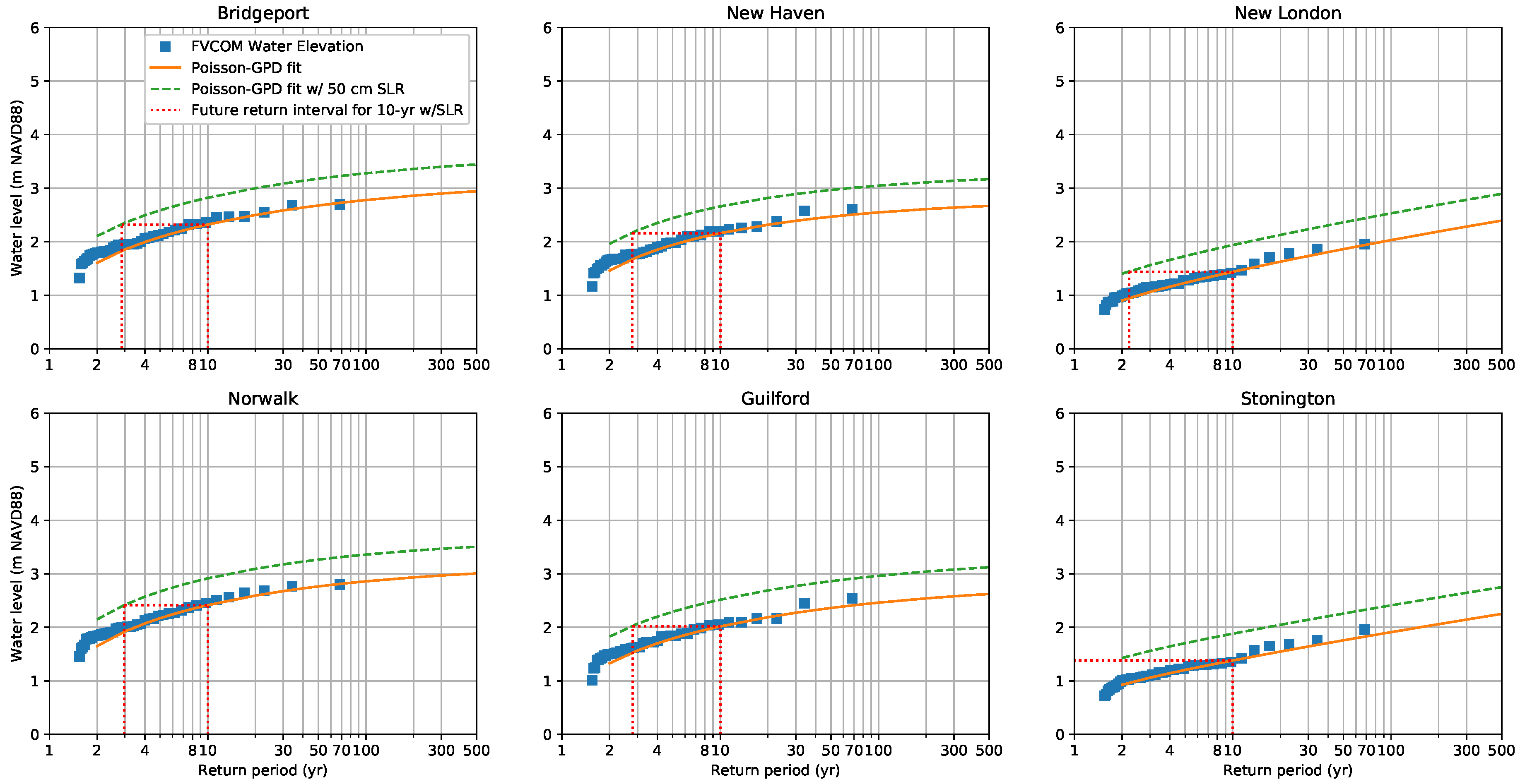
4.6. Sea Level Rise Projections

The future projection of greenhouse gas emissions and the response of atmospheric and oceanic temperatures influence the uncertainties related to estimates of sea-level rise [51]. Any sea-level rise will, however, reduce the return period estimates. In order to better understand the effects of sea-level rise on the risk assessments, a planning threshold of 50 cm sea level rise by the year 2050 [6] is added to the initial level of the Poisson-GPD fit (Figure 10). The green dashed line in the figure shows the future return periods for 2050, assuming the storm characteristics remain constant (the distribution of the shape and scale parameters). The fitting was then repeated to find the corresponding return intervals for the same water levels. The results indicate that the water levels estimated for a 10-year storm (10% annual probability) would occur with a 2-year return period (

Table 6. Projected return periods for the current 10-year storm for the year 2050 with 50 cm sea level rise.

Town	Water Level of Current 10-Year Storm (M)	Return Period with 50 Cm Sea Level Rise (Years)
Bridgeport	2.32	2.86
New Haven	2.16	2.78
New London	1.44	2.21
Norwalk	2.41	2.97
Guilford	2.02	2.79
Stonington	1.38	<2

). These changes in the annual probabilities due to sea-level rise also differ based on location. Likewise, what would currently be considered a 100-year storm event (1% annual probability) would become a 20-year event. However, given the large uncertainty ranges surrounding the estimates of each return level curve, estimating rarer storms with longer return periods is not recommended due to larger uncertainties in SLR projections.

5. Conclusions

This paper is intended as a guide for decision-makers to identify risk probabilities for the coastal protection project design for the current environment, as well as considering local sea-level rise projections for 2050. This study provides modeled water levels and significant wave heights in LIS to improve probability estimates of the extreme surge and wave heights for Connecticut shorelines and municipalities, filling the gaps between very sparse coastal observations. We analyzed 68 years of data with POT to model the 44 highest-ranked storms. We then estimated 10-, 30-, 50-, and 100-year return period water levels and significant wave heights for all Connecticut coastal towns. It is worth noting that the Poisson-GPD distribution best fits the empirical distribution.

The model results show that the water levels for a given return period are higher along the western end of the Connecticut coast than the eastern end. Conversely, significant wave heights increase eastward. The results lie within the confidence interval of the previous NACCS study and show good agreement with tide gauge and buoy observations. The 1% annual exceedance probabilities of water levels in Bridgeport, New Haven, and New London is 2.78 m, 2.55 m, and 2.03 m, respectively, and the corresponding significant wave heights are 4.48 m, 3.98 m, and 4.91 m. The probability of the occurrence of extreme events increases when a 0.5 m local sea-level rise projection for 2050 is included in our calculations. When a 0.5 m sea-level rise is included, a 10% annual probability event (10-year return period) increases to a 50% annual probability (2-year return period) and a 1% annual probability event (100-year return period) increase to a 5% annual probability (20-year return period). Although this study presents annual probabilities for storm surges and significant wave heights of the next few decades, the potential for climate change to impact these probabilities must be considered in planning coastal projects. Since the degree of sea-level rise will significantly affect these results, we feel it is imperative to repeat coastal flood risk assessments as better predictions of sea level rise become available.

References

1. Dixon, K. Sandy Storm Damage Tops $360M in State. Connecticut Post, 14 November 2012. Available online: https://www.ctpost.com/news/article/Sandy-storm-damage-tops-360M-in-state-4037538.php (accessed on 26 June 2020).
2. Cooper, M.J.; Beevers, M.D.; Oppenheimer, M. The potential impacts of sea level rise on the coastal region of New Jersey, USA. Clim. Chang. 2008, 90, 475–492. [Google Scholar] [CrossRef]
3. Kirshen, P.; Knee, K.; Ruth, M. Climate change and coastal flooding in Metro Boston: Impacts and adaptation strategies. Clim. Chang. 2008, 90, 453–473. [Google Scholar] [CrossRef]
4. Hunter, J. A simple technique for estimating an allowance for uncertain sea-level rise. Clim. Chang. 2012, 113, 239–252. [Google Scholar] [CrossRef]
5. Tebaldi, C.; Strauss, B.H.; Zervas, C.E. Modelling sea level rise impacts on storm surges along US coasts. Environ. Res. Lett. 2012, 7, 014032. [Google Scholar] [CrossRef]
6. O’Donnell, J. Sea Level Rise in Connecticut; Technical Report; Connecticut Institute for Resilience & Climate Adaptation: Groton, CT, USA, 2013. [Google Scholar]
7. Cialone, M.; Massey, T.; Anderson, M.; Grzegorzewski, A.; Jensen, R.; Cialone, A.; Mark, D.; Pevey, K.; Gunkel, B.; McAlpin, T. North Atlantic Coast Comprehensive Study (NACCS) Coastal Storm Model Simulations: Waves and Water Levels; Technical Report; Engineer Research and Development Center: Vicksburg, MS, USA, 2015. [Google Scholar]
8. FEMA. Wave Height Analysis for Flood Insurance Studies; Technical Documentation for WHAFIS Program Version 3.0; Federal Emergency Management Agency: Washington, DC, USA, 1988.
9. Nadal-Caraballo, N.C.; Melby, J.A. North Atlantic Coast Comprehensive Study Phase I: Statistical Analysis of Historical Extreme Water Levels with Sea Level Change. J. Coast. Res. 2015, 32, 35–45. [Google Scholar]
10. Ho, F.P.; Myers, V.A. Joint Probability Method of Tide Frequency Analysis Applied to Apalachicola Bay and St. George Sound, Florida; Technical Report; National Weather Service: Washington, DC, USA, 1975. [Google Scholar]
11. Resio, D.T.; Boc, S.J.; Borgman, L.; Cardone, V.; Cox, A.T.; Dally, W.R.; Dean, R.G.; Divoky, D.; Hirsh, E.; Irish, J.L.; et al. White Paper on Estimating Hurricane Inundation Probabilities; US Army Corps of Engineers: Vicksburg, MI, USA, 2007. [Google Scholar]
12. Toro, G.R.; Resio, D.T.; Divoky, D.; Niedoroda, A.W.; Reed, C. Efficient joint-probability methods for hurricane surge frequency analysis. Ocean Eng. 2010, 37, 125–134. [Google Scholar] [CrossRef]
13. Komen, G.J.; Cavaleri, L.; Donelan, M.; Hasselmann, K.; Hasselmann, S.; Janssen, P.A.E.M. Dynamics and Modelling of Ocean Waves; Cambridge University Press: Cambridge, UK, 1994; p. 532. [Google Scholar]
14. Massey, T.C.; Anderson, M.E.; Smith, J.M.; Gomez, J.; Jones, R. STWAVE: Steady-State Spectral Wave Model User’s Manual for STWAVE, Version 6.0; Technical Report; US Army Engineer Research and Development Center: Vicksburg, MS, USA, September 2011. [Google Scholar]
15. Luettich, R.A.; Westerink, J.J.; Scheffner, N.W. ADCIRC: An Advanced Three-Dimensional Circulation Model for Shelves, Coasts, and Estuaries; Technical Report; U.S. Army Engineer Research and Development Center: Vicksburg, MS, USA, 1992. [Google Scholar]
16. Bilskie, M.V.; Hagen, S.C.; Medeiros, S.C.; Passeri, D.L. Dynamics of sea level rise and coastal flooding. Geophys. Res. Lett. 2014, 41, 927–934. [Google Scholar] [CrossRef]
17. Lin, Y.; Fissel, D.B. High resolution 3-d finite-volume coastal ocean modeling in lower campbell river and discovery passage, British Columbia, Canada. J. Mar. Sci. Eng. 2014, 2, 209–225. [Google Scholar] [CrossRef]
18. Kopp, R.E.; Horton, R.M.; Little, C.M.; Mitrovica, J.X.; Oppenheimer, M.; Rasmussen, D.J.; Strauss, B.H.; Tebaldi, C. Probabilistic 21st and 22nd century sea-level projections at a global network of tide-gauge sites. Earth’s Future 2014, 2, 383–406. [Google Scholar] [CrossRef]
19. Pullen, T.; Allsop, N.W.H.; Bruce, T.; Kortenhaus, A.; Schüttrumpf, H.; van der Meer, J.W. EurOtop Wave Overtopping of Sea Defences and Related Structures: Assessment Manual; Technical Report 73; 2007. Available online: http://www.overtopping-manual.com/eurotop/downloads/ (accessed on 26 June 2020).
20. O’Donnell, J.; Wilson, R.E.; Lwiza, K.; Whitney, M.; Bohlen, W.F.; Codiga, D.; Fribance, D.B.; Fake, T.; Bowman, M.; Varekamp, J. The Physical Oceanography of Long Island Sound. In Long Island Sound; Springer: New York, NY, USA, 2014; pp. 79–158. [Google Scholar] [CrossRef]
21. O’Donnell, J.; O’Donnell, J.E. Coastal vulnerability in Long Island Sound: The spatial structure of extreme sea level statistics. In Proceedings of the OCEANS 2012 MTS/IEEE: Harnessing the Power of the Ocean, Hampton Roads, VA, USA, 14–19 October 2012; pp. 1–4. [Google Scholar] [CrossRef]
22. Fribance, D.B.; Donnell, J.O.; Bohlen, W.F.; Houk, A. Tides and Overtides in Long Island Sound. J. Mar. Res. 2010, 68, 1–35. [Google Scholar] [CrossRef]
23. NOAA. Tides and Currents. Available online: https://tidesandcurrents.noaa.gov/ (accessed on 26 June 2020).
24. NOAA. National Data Buoy Center. Available online: https://www.ndbc.noaa.gov/ (accessed on 26 June 2020).
25. NOAA National Center for Environmental Information. Local Climatological Data (LCD) Dataset. Available online: https://www.ncdc.noaa.gov/cdo-web/datatools/lcd (accessed on 26 June 2020).
26. Northeastern Regional Association of Coastal Ocean Observing Systems. Long Island Sound Coastal Observatory. 1999. Available online: https://mysound.uconn.edu/ (accessed on 26 June 2020).
27. Chen, C.; Beardsley, R.; Cowles, G. An Unstructured Grid, Finite-Volume Coastal Ocean Model (FVCOM) System. Oceanography 2006, 19, 78–89. [Google Scholar] [CrossRef] [Green Version]
28. Qi, J.; Chen, C.; Beardsley, R.C.; Perrie, W.; Cowles, G.W.; Lai, Z. An unstructured-grid finite-volume surface wave model (FVCOM-SWAVE): Implementation, validations and applications. Ocean Model. 2009, 28, 153–166. [Google Scholar] [CrossRef]
29. Booij, N.; Ris, R.C.; Holthuijsen, L.H. A third-generation wave model for coastal regions: 1. Model description and validation. J. Geophys. Res. Ocean. 1999, 104, 7649–7666. [Google Scholar] [CrossRef] [Green Version]
30. Wu, L.; Chen, C.; Guo, P.; Shi, M.; Qi, J.; Ge, J. A FVCOM-based unstructured grid wave, current, sediment transport model, I. Model description and validation. J. Ocean Univ. China 2011, 10, 1–8. [Google Scholar] [CrossRef]
31. O’Donnell, J.; McCardell, G.; Berger, L. Physical Oceanography of Eastern Long Island Sound Region: Modeling; Appendix C-2; Technical Report, Supplemental Environmental Impact Statement for the Designation of Dredged Material Disposal Sites in Eastern Long Island Sound, Connecticut and New York; University of Connecticut: Groron, CT, USA, 2016. [Google Scholar] [CrossRef]
32. Cowles, G.W.; Lentz, S.J.; Chen, C.; Xu, Q.; Beardsley, R.C. Comparison of observed and model-computed low frequency circulation and hydrography on the New England Shelf. J. Geophys. Res. Ocean. 2008, 113. [Google Scholar] [CrossRef] [Green Version]
33. Chen, C.; Huang, H.; Beardsley, R.C.; Xu, Q.; Limeburner, R.; Cowles, G.W.; Sun, Y.; Qi, J.; Lin, H. Tidal dynamics in the Gulf of Maine and New England Shelf: An application of FVCOM. J. Geophys. Res. Ocean. 2011, 116. [Google Scholar] [CrossRef] [Green Version]
34. Chawla, A.; Spindler, D.; Tolman, H. WAVEWATCH III Hindcasts with Re-Analysis Winds. Initial Report on Model Setup; Technical Report, NOAA/NWS/NCEP/MMAB Tech. Note 291; U. S. Department of Commerce: Camp Springs, MD, USA, 2011.
35. Spindler, D.; Chawla, A.; Tolman, H.L. An Initial Look at the CFSR Reanalysis Winds for Wave Modeling; Technical Report, NOAA/NWS/NCEP/MMAB Tech. Note 290; U. S. Department of Commerce: Camp Springs, MD, USA, 2011.
36. Weibull, W. A Statistical Theory of the Strength of Materials; Handlingar/Ingeniörsvetenskapsakademien, Generalstabens Litografiska Anstalts Förlag: Stockholm, Sweden, 1939. [Google Scholar]
37. Davison, A.C.; Smith, R.L. Models for Exceedances Over High Thresholds. J. R. Stat. Soc. Ser. B (Methodol.) 1990, 52, 393–425. [Google Scholar] [CrossRef]
38. Brodtkorb, P.A.; Johannesson, P.; Lindgren, G.; Rychlik, I.; Ryden, J.; Sjo, E. WAFO—A Matlab toolbox for analysis of random waves and loads. In Proceedings of the International Offshore and Polar Engineering Conference, Seattle, WA, USA, 28 May–2 June 2000; Volume 3, pp. 343–350. [Google Scholar]
39. Finkenstadt, B.; Rootzen, H. Extreme Values in Finance, Telecommunications, and the Environment; Chapman & Hall/CRC Monographs on Statistics & Applied Probability; Taylor & Francis: Oxford, UK, 2003. [Google Scholar]
40. Silva, A.T.; Naghettini, M.; Portela, M.M. On some aspects of peaks-over-threshold modeling of floods under nonstationarity using climate covariates. Stoch. Environ. Res. Risk Assess. 2015, 30, 207–224. [Google Scholar] [CrossRef]
41. Makkonen, L. Plotting Positions in Extreme Value Analysis. J. Appl. Meteorol. Climatol. 2006, 45, 334–340. [Google Scholar] [CrossRef]
42. Hanna, S.R.; Heinold, D.W. Development and Application of a Simple Method for Evaluating Air Quality Models; Number 4409; American Petroleum Institute: Washington, DC, USA, 1985. [Google Scholar]
43. Willmott, C.J. On the validation of models. Phys. Geogr. 1981, 2, 184–194. [Google Scholar] [CrossRef]
44. Cunnane, C. A note on the Poisson assumption in partial duration series models. Water Resour. Res. 1979, 15, 489–494. [Google Scholar] [CrossRef]
45. Northeast Regional Ocean Council. NACCS Coastal Storm and Flood Risk Data. Available online: https://cdm16021.contentdm.oclc.org/digital/collection/p16021coll10/id/9411 (accessed on 26 June 2020).
46. Kalnay, E.; Kanamitsu, M.; Kistler, R.; Collins, W.; Deaven, D.; Gandin, L.; Iredell, M.; Saha, S.; White, G.; Woollen, J.; et al. The NCEP/NCAR 40-Year Reanalysis Project. Bull. Am. Meteorol. Soc. 1996, 77, 437–471. [Google Scholar] [CrossRef] [Green Version]
47. Mesinger, F.; DiMego, G.; Kalnay, E.; Mitchell, K.; Shafran, P.C.; Ebisuzaki, W.; Jović, D.; Woollen, J.; Rogers, E.; Berbery, E.H.; et al. North American Regional Reanalysis. Bull. Am. Meteorol. Soc. 2006, 87, 343–360. [Google Scholar] [CrossRef] [Green Version]
48. Garvine, R.W. A simple model of estuarine subtidal fluctuations forced by local and remote wind stress. J. Geophys. Res. 1985, 90, 11945. [Google Scholar] [CrossRef]
49. Wong, K.C. Sea Level Variability in Long Island Sound. Estuaries 1990, 13, 362. [Google Scholar] [CrossRef]
50. Whitney, M.M.; Codiga, D.L. Response of a Large Stratified Estuary to Wind Events: Observations, Simulations, and Theory for Long Island Sound. J. Phys. Oceanogr. 2011, 41, 1308–1327. [Google Scholar] [CrossRef]
51. IPCC. IPCC Climate Change 2014: Synthesis Report. Contribution of Working Groups I, II and III to the Fifth Assessment Report of the Intergovernmental Panel on Climate Change; Technical Report; Pachauri, R.K., Meyer, L.A., Eds.; IPCC: Geneva, Switzerland, 2014. [Google Scholar] [CrossRef] [Green Version]
Figure 1. Model domain, mesh, and bathymetry (color ramp) of the Long Island Sound FVCOM-SWAVE model, and locations of NOAA tide gauge stations (green squares), buoys (red triangles), airports (yellow airplane symbols) and coastal points (blue stars) where model results are evaluated.
Jmse 08 00475 g001
Figure 2. Comparison of water level (left) and significant wave height (right) time series between model and observation during hurricane Sandy (a) and Irene (b).
Jmse 08 00475 g002
Figure 3. Comparison of water level time series between model (blue) and storm surge sensors from USGS (orange) during hurricane Sandy (a) and Irene (b).
Jmse 08 00475 g003
Figure 4. Comparison of observed and modeled peak values for water level (left) and significant wave height (right) at tide gauge stations and buoys during storm events.
Jmse 08 00475 g004
Figure 5. Return periods of observed and modeled water level (a) and significant wave height (b) at the location of observations.
Jmse 08 00475 g005
Figure 6. Estimated return level (colored contour) and return period (vertical axis) for water level (a) and significant wave height (b) evaluated at 24 locations down estuary along the Connecticut coast. The point numbers increase from west to east, 1 indicates Greenwich, whereas 24 is Stonington.
Jmse 08 00475 g006
Figure 7. The water level and return period plots for Bridgeport, New Haven, and New London.
Jmse 08 00475 g007
Figure 8. The significant wave height and return period plots for Bridgeport, New Haven, and New London.
Jmse 08 00475 g008
Figure 9. The average error of 100-year water level between model and FEMA estimates. Red indicates that model values are higher than FEMA.
Jmse 08 00475 g009
Figure 10. The water level projection for the year 2050 upper bound of 50 cm sea level rise.
Jmse 08 00475 g010