A Comparison of Numerical Simulations and Model Experiments on Parametric Roll in Irregular Seas

Abstract

The recently finalised Second Generation Intact Stability Criteria (SGISC), produced by the International Maritime Organisation (IMO), contain a level 3 assessment, the so-called Direct Stability Assessment (DSA). This assessment can be carried out using either model experiments or simulations. The fact that such a choice is given implies that the methods are equivalent in accuracy. This assumption has been verified, for one case, by the Cooperative Research Ships (CRS) community. The verification was based on new model experiments and calculated results, using four different programs owned by different CRS members. Results of the verification of the parametric roll failure mode in regular waves were published before, but this study concerns results in irregular seas. The experimental and numerical results are compared in both probabilistic and deterministic manners. The probabilistic comparison showed that the simulation programs considered are sometimes conservative and sometimes non-conservative in the prediction of the probability of an extreme value. The deterministic comparison in head seas showed that parametric roll events were predicted in the simulations in a wave train that showed no sign of important roll events in the measurement. The deterministic comparison in the following seas, on the other hand, showed an accurate fit of experimental and numerical results. It is suggested that predictions could possibly be improved by adding non-linear diffraction forces to the numerical model.

Nomenclature

Symbol	Unit	Description
Aφφ	ton.m2	Roll added moment of inertia
B	m	Beam
B1	kNms	Linear component of roll damping
B2	kNms2	Quadratic component of roll damping
B3	kNms3	Cubic component or roll damping
BCR	kNms	Critical roll damping
Cφφ	kNm	Roll restoring moment
Fn	-	Froude number, $Fn=v/\sqrt{gL}$
F4	kNm	4th component of force (roll moment)
F4a	kNm	Amplitude of roll moment
g	m/s2	Acceleration due to gravity
GM	m	Transverse metacentric height
Hs	m	Significant wave height
Iφφ	ton.m2	Roll moment of inertia
KG	m	Height Centre of Gravity (CoG) above keel
Lpp	m	Length between perpendiculars
t	s	time
tP-ENV	s	Time instant of the peak of a parametric roll event in a roll angle signal
T	m	Draft
Tp	s	Peak period of the wave spectrum
Tφ	s	Roll natural period
kxx	m	Roll gyradius
kxx *	m	Roll gyradius including added mass
kYY	m	Pitch gyradius
p	-	Linear roll damping coefficient
q	-	Quadratic roll damping coefficient
r	-	Cubic roll damping coefficient
Vs	kn	Ship speed
Vs-av	kn	Average ship speed in a sea state
γ	-	Peakedness parameter of Jonswap wave spectrum
Δ	ton	Displacement
ε	rad	Phase angle
ζa	m	Wave amplitude
φ	rad	Roll angle
φa	rad	Roll angle amplitude
ω0	rad/s	Earth fixed wave frequency
ωe	rad/s	Wave-encounter frequency

1. Introduction

As the Second Generation Intact Stability Criteria (SGISC) are now in the final phase, it is now the appropriate time to verify if existing simulation tools are indeed ready for a Level 3 assessment, also called Direct Stability Assessment. A number of basis criteria have been defined by the International Maritem Organization (IMO) Intact Stability Correspondence Group [1], and finalised during a session of the IMO sub-committee on Ship Design and Construction (SDC-7) [2], but these criteria do not guarantee the certain accuracy of the simulations versus the results of experiments. Work has been done in the Cooperative Research Ships (CRS) [3] consortium, which has focused on three out of five stability failure modes: parametric roll, loss of stability and dead ship. This paper focusses on the results for parametric roll in irregular seas. Results in regular waves have been presented before [4]. As in the earlier publication, the results of different simulation programs have been compared to the results of experiments.

Amongst the identified dynamic stability failure mode, parametric roll is probably the most emblematic and the most well-known. Parametric rolling (a parametric resonance phenomenon) is an amplification of roll motions caused by the periodic variation of transverse stability in waves [4]. It is known that parametric roll is mostly expected to occur in head, following, bow and stern quartering seas, when the wave-encounter frequency is approximately twice the natural roll frequency, and the stability variations are large. The consequence of this last requirement is that the wave-length is in the order of the ship length. Additional to this, the roll damping of the ship should be low, so that it is insufficient to dissipate the additional energy accumulated because of the parametric resonance. Since roll damping increases significantly with speed, the phenomenon is more likely to occur at low speeds.

This work adds to existing benchmark cases, like those published by France et al. [5], Spanos and Papanikolaou [6], and Reed [7]. The added value of this work is the effort put into accurately determining roll damping, for larger amplitudes as well, and in the availability of results concerning both regular waves and irregular seas. In particular, the experimental work done to determine the roll damping is valuable, in our opinion.

The prediction of roll damping is notably problematic. Estimation formulas are usually based on the work by Ikeda and colleagues [8,9,10,11,12,13]. This method has known shortcomings, but it is the best method available. More recently, CFD has been used to estimate the roll damping, and this method has been shown to give good results [14]. It is noted here that an inaccurate estimation of the roll damping dominates the results from further simulations on most of the stability failure modes defined by the IMO. This problem has been circumvented in this publication by using the experimentally determined roll damping in the numerical simulations. Roll decay simulations have been carried out to check on double counts.

The vessel used in this study is the KCS hull form. This vessel has already been used in several parametric roll studies [15,16,17]. Yu et al. [15,16] worked on the sensitivity of the KCS to parametric roll in regular waves for a large number of speeds. Experiments were carried out and analysed to test an early detection algorithm for parametric roll. Interestingly, they showed that parametric roll occurred mainly for speeds 0.05 < Fn < 0.13, but this depends largely on the chosen natural roll period (which was 21.6 s for the full-scale vessel). Ruiz et al. [17] studied parametric roll in shallow water by means of experiments. They checked the ABS prediction formula [18] and found it to be conservative; it incorrectly predicted parametric roll in 3 out of 12 cases, and 9 predictions were correct. The 3 degree of freedom (DoF) numerical model developed by Neves et al. [19] performed slightly better, with 2 “false positives” and 10 correct predictions.

The focus of this work is on a comparison of the simulation programs “as is”; no effort has been put into improving the numerical models implemented in the various simulation programs. However, suggestions for improvements are made in this publication.

2. Experiments

The hull form of the KCS is fully specified on the SIMMAN2008 website [20]. A wooden model has been built at a scale ratio of 37.89 according to these lines. This model was equipped with bilge keels, height—0.40 m, length—68.82 m in full scale (St 6–14), and a rudder (span—9.90 m, mean chord—5.54 m in full scale). The main dimensions of the ship and the loading conditions are given in

Table 1. Main dimensions and loading conditions of the KCS for the parametric roll experiments. LC-1 has been used for experiments in head seas, LC-2 for experiments in following seas.

Parameter	Symbol	LC-1	LC-12	Units
Length perp.	Lpp	230.00		m
Beam	B	32.20		m
Draft	T	10.80		m
Depth	D	19.00		m
Displacement	Δ	53,389		ton
Vertical CoG	KG	13.67	14.34	m
Metacentric height	GM	1.22	0.60	m
Roll nat. period	Tφ	23.6	34.1	s
Roll gyradius	kXX	11.90		m
Pitch gyradius	kYY	57.50		m
Yaw gyradius	kZZ	57.50		m

. Two loading conditions (LC) have been used: LC-1 for the experiments and simulations in head seas, LC-12 for the following seas cases.

The experiments were carried out in the Seakeeping and Manoeuvring Basin of MARIN (170 × 40 × 5 m), with a free running model; only thin electric cables connected the model to the carriage. The model maintained heading using an autopilot that controlled the rudder. The duration of the experiments in each of the presented conditions amounted to 3 h. To realise this, a long time trace for the wave generator was made. The actual experiments with the model were done in parts, due to the limited length of the basin. Subsequent runs used subsequent parts of the 3-h wave signal. The length of the individual runs was typically 5300 m (full scale value).

The wave spectra generated for the experiments were based on the JONSWAP formulation [21] for the distribution of the energy over the wave frequency. These spectra are characterised by the period of the peak of the spectrum Tp, the significant wave height Hs and the peak enhancement factor γ. The first two parameters were varied for the different tests, but the peak enhancement factor was fixed at γ = 3.3. An overview of the conditions in which the tests were done is presented in paragraph 6.

A deterministic comparison requires reliable information on the incoming wave, that is, without disturbances from the model. For experiments in head seas, the wave probe in front of the model can be used for this purpose, but the wave probes before and aft of the model measure the presence of the model in the following seas. Therefore, a few runs were selected for a re-measurement of the wave without the model being present. These are the runs that have been used in the deterministic comparison.

3. Numerical Methods

Four different simulation programs have been used in this paper; two owned by different class societies, and two by different research organisations. The programs have identical basics: the hydrodynamics are calculated by a linear potential flow theory, and the linear restoring and excitation due to the incoming wave are replaced by non-linear Froude–Krylov and restoring forces. Other characteristics of the programs have been summarised in

Table 2. Characteristics of the simulation programs (Sim 1–4) used in this study.

Characteristic	Sim-1	Sim-2	Sim-3	Sim-4
Wave model	L	L	L	L
DoF	6	6	6	6
Speed control	S	C	C	C
Hydrodynamics	R	ZG	S	ZG
Rel. motion	I	I	I	I
Pressure for z > 0	H	H	HW	HW
Pressure integration	M	M	M	M
Course control	SD	F	R	R

.

All programs have used linear waves (L) and assumed 6 Degrees of Freedom (DoF). For all simulations, the speed was kept constant (C), or first order surge motions were allowed by means of a soft spring system (S). The hydrodynamic models used Rankine source panels (R), zero speed Green functions with an encounter frequency correction (ZG) or strip theory (S). To determine the wetted surface, the relative motion was based on ship motions and the incoming wave only (I). The pressure above the calm water surface (z > 0) is usually determined by the hydrostatic pressure (H). In two cases (Sim 3, 4) Wheeler stretching [22] was added to the dynamic pressure component (HW). All programs used a mesh (M) for the pressure integration. Course control was realised by springs and dampers (SD), by freezing the yaw degree of freedom (F), or by a rudder controlled via an autopilot (R).

A critical aspect is normally the determination of the roll damping. An estimate is usually based on Ikeda’s method; nowadays, CFD is also being used. One program can use a translation of the Ikeda method to the time domain to better capture non-linear effects. For the work presented in this article, the results of experiments were used in a second or third order damping model by all simulation programs.

Simulations in the specified sea states were carried out for all four programs; statistical results are compared in further paragraphs. The additional work to perform the deterministic comparison was only done using programs Sim-2 and Sim-3.

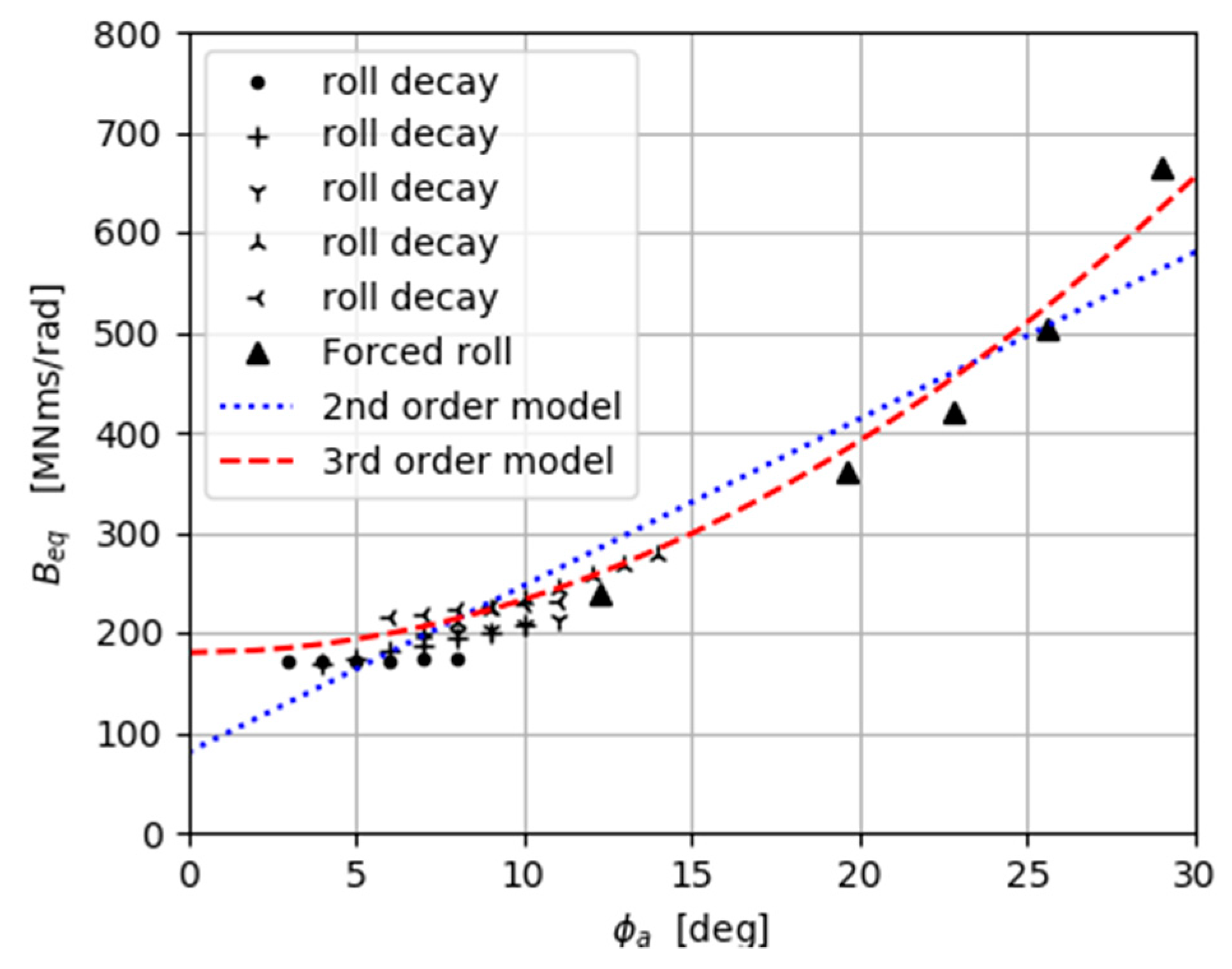
4. Results of Roll Decay and Forced Roll Tests

Quite some effort was spent on measuring the roll damping, since this is a critical parameter in parametric roll predictions, and, in fact, in most of the SGISC failure modes. Roll decay experiments were carried out at different speeds and different initial angles, repeat experiments were done for critical cases, and forced roll experiments were done. This latter experiment was carried out by fitting an electrical motor with a flywheel inside the model. This motor was mounted on a 6 DoF force balance. The motor had a rotation axis in the longitudinal direction of the model, and was forced in a harmonically changing rotation rate. The rotational acceleration of the flywheel provided the roll moment. Experiments were done with various amplitudes, all at the natural roll frequency for the two loading conditions.

Roll decay tests were performed for different initial angles (6°, 12° and 15°), and several repeat tests were done. They were analysed using a fitting procedure for a third order, 1 DoF roll damping model [Equation (1)], an extension of the second order model proposed by Lewandowski [23]. Note that the restoring moment in Equation (1) is defined by just the linear (hydrostatic) coefficient.

The forced roll tests were performed with different values for the roll moment, all at the roll resonance frequency. The experiments were analysed using the roll moment measured by the 6 DoF force balance, and using the phase angle between the roll motion and the moment produced by the motor.

$$\left(I_{\phi \phi }+A_{\phi \phi }\right)\ddot{\phi }+B_1\dot{\phi }+B_2\dot{\phi }\left|\dot{\phi }\right|+B_3{\dot{\phi }}^3+C_{\phi \phi }\phi =0$$

(1)

The damping parameters B₁, B₂ and B₃ are expressed in non-dimensional coefficients p, q and r. These coefficients are defined in Equation (2). These definitions make use of the critical roll damping B_CR that is defined in Equation (3). Values for the non-dimensional damping coefficients as derived from the experiments are listed in

Table 3. Choice of p, q and r coefficients for the simulations.

Vs [kn]	Loading Condition	Tφ [s]	BCR [kNms]	p [-]	q [1/°]	r [1/°2]
0	LC-1	23.6	4.77 × 106	0	2.35 × 10-2	0
				5.00e−02	0	8.5 × 10-4
8		23.0	4.69 × 106	1.07e−01	2.30 × 10-2	0
				2.40e−01	0	7.0 x10-4
8	LC-12	32.7	3.33 × 106	9.40e−02	2.50 × 10-2	0

. Note that, for some conditions, the coefficients for a second order as well as for a third order model are given.

$$B_1=\frac{p}{2\pi }{B}_{CR}, B_2=\frac{3q{T}_{\phi }}{32\pi }{B}_{CR}, B_3=\frac{r{T}_{\phi }{}^2}{6{\pi }^2}{B}_{CR}$$

(2)

$$B_{CR}=2\Delta k_{XX}\sqrt{gGM}$$

(3)

The results of the roll damping experiments at Vs = 8 kn are shown in Figure 1. This figure shows the results of the roll decay tests up to a maximum roll angle of 15°, and the results of forced oscillation tests in the range 12° < φ < 29°. The two methods give consistent results. It was concluded that the forced roll experiment is a very suitable method for determining the damping at large amplitudes.

Figure 1 also demonstrates a fundamental problem; it is not possible to accurately model the roll damping over the full amplitude range with just a quadratic model. The plot shows the equivalent linear damping as a function of the roll amplitude, so a quadratic roll damping model, as defined in Equation (1), is displayed as a straight line. A third order model gives a much better fit to the experimental data, as is also shown in the figure. Note that the use of either the second or the third order model has a large effect on the limit of the roll damping for $\phi \to 0$. It was expected that the onset of parametric roll would be affected by this limit.

5. Probabilistic Analysis of Results

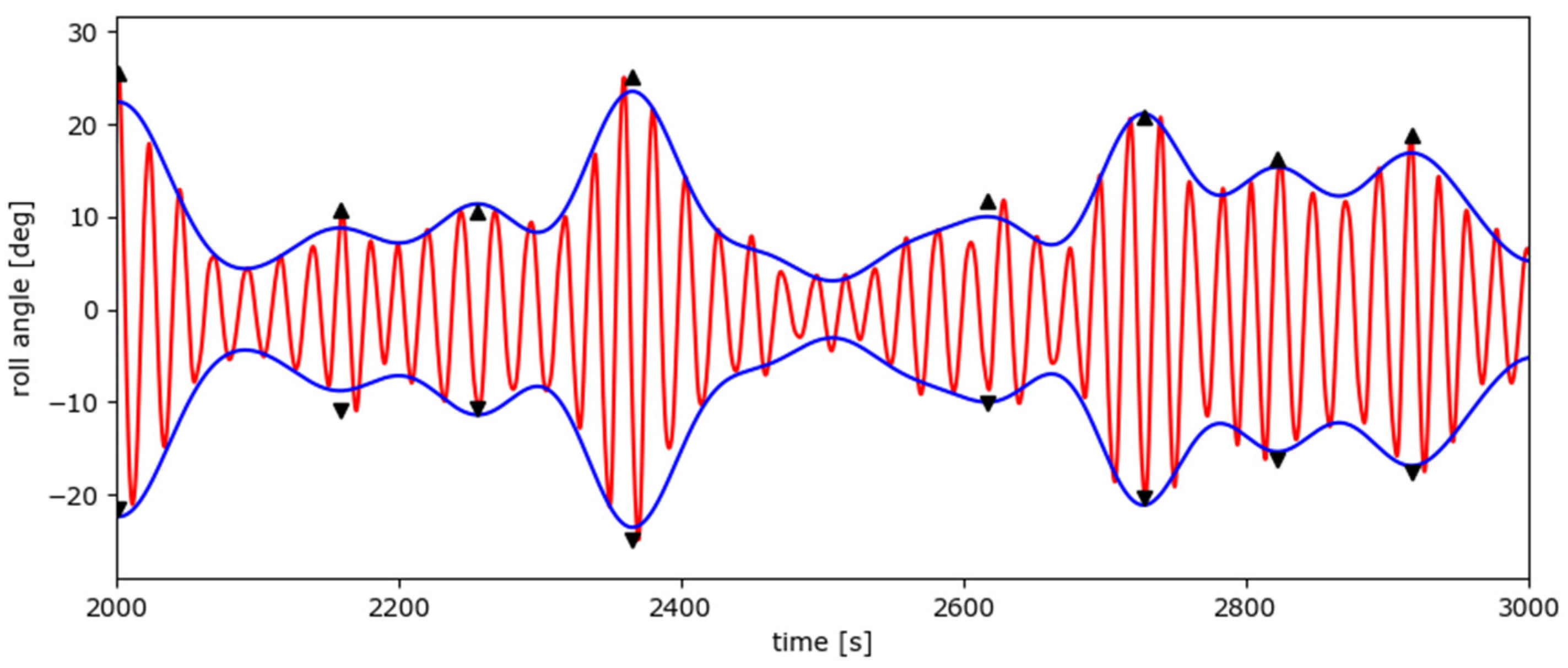
5.1. Analysis of Parametric Roll Events

A first analysis aimed at considering the number of parametric roll events and characterising each event by its maximum roll angle. In order to identify these events, a Hilbert transform was made of the roll signal, and this function was filtered by a low-pass filter with frequencies 0.05 and 0.10 rad/s. Signals with a frequency below the first value fully pass the filter; signals with a frequency in-between the two values are partly filtered, and signals with a frequency higher than the highest values do not pass the filter. The filtered Hilbert transform can be considered as the envelope of the roll signal, thus identifying parametric roll events. These events are further identified by the time instant of the peak of the envelope t_P-ENV. The actual peak is the peak of the roll signal in the interval defined in Equation (4). The result of this procedure is illustrated in Figure 2.

$$t_{P-ENV}-T_{\phi }<t<t_{P-ENV}+T_{\phi }$$

(4)

Using this analysis, the ensemble statistics have been made from parametric roll events classed in bins of 5°, starting at 10° roll amplitude. As an example, the results for the simulations done by program Sim-2 are given in Figure 3. The results show that convergence, in terms of the number of events/h, is slow. The figure suggests that only the last five bars show little changes, meaning that 15 simulations of 3 h each are necessary for convergence. It is concluded that results from one 3-h simulation (and hence also from the 3-h experimental results) have a large uncertainty margin.

5.2. Analysis of Extreme Roll Angles

A probability of exceedance plot can be made from the local extreme values of the roll motion. An extreme value has been defined as the maximum positive value between two subsequent zero up-crossings. Such a plot contains both related events (belonging to the same parametric roll event) and unrelated events. From a statistical point of view, this is not a nice property, but it has been argued by Wandji [24] that the peak values are unrelated.

Figure 4 and Figure 5 show the extreme value distributions of the roll motions for two sea states, from the programs Sim-1 and Sim-4. The figures show the extreme value distributions for 10 realisations of each sea state. The mean (solid black circles with dotted lines) and the 95% confidence intervals (solid red lines) were obtained from the 10 realisations per case. Extreme roll values smaller than 3° were ignored while obtaining the probabilities. These two examples show cases with a small and a larger confidence interval.

It can be observed that there is an inherent variability in the distributions. This variability seems to depend on the programs and the sea states. In general, the simulations exhibit wider spreads for the large roll angles. This can be observed especially in the trends of the confidence intervals. Overall, the two programs produce similar results for both sea states

5.3. Deterministic Analysis of Results

A deterministic comparison of the numerical and experimental results needs some special care. The experiments were carried out using a free running model, so the speed was not constant. The speed variations in the experiment and in the simulation are usually different, so after a short while the synchronisation of the wave experienced by the physical and the numerical model will be off. The method chosen to compensate for this involves the numerical model using the wave as measured on the location of the physical model in the tank at the subject time instant. This approach was introduced by van Walree and de Jong [25]. The solutions of the equations of motion, and hence the accelerations and velocities, was not adapted.

When simulations are carried out in exactly long-crested head or following seas, it is necessary to give some small disturbance in the lateral direction to initiate the roll excitation and hence the motion. Two methods were tried; the first is to give a small heel angle (0.1°) early in the simulation (at t = 10 s) and the second is to do the simulation in a heading of 179° or 179.5°, rather than 180°. The results proved that both methods work and give identical results.

6. Overview of Experimental Results

The conditions in which the experiments were carried out have been summarised in

Table 4. Overview of tested wave conditions.

Wave Direction	Av. ship Speed Vs-av [kn]	Sign. Wave Height Hs [m]	Peak Period Tp [s]	Peakedness Parameter γ [-]	Test Duration [h]
Head	7.6	7.0	13.5	3.3	3
	7.9	8.0
Following	7.9	4.0	13.5	3.3	3

. An overview of the results of the experiments in head and following seas has been made in Figure 6. The figure shows the distributions of the extreme roll values and the number of parametric roll events divided in different amplitude classes. The first figure also features three-parameter Weibull fits that are normally used for extreme value predictions. Noted again is the fact that the loading condition of the vessel is different for the head seas and the following seas cases.

This figure shows some interesting results. Although the roll angles in the 8-m sea state are on average larger than in the 7-m sea state, the opposite appears to be true for the extreme values. The distributions of the parametric roll events are quite different in these two sea states. The lower sea state shows many events with a low amplitude, and the number of events is steadily decreasing for the higher amplitude classes. This is not the case in the higher sea state; there is a strong peak of events with a maximum amplitude of 20°–25°.

The trends in following seas show a similar distribution of the parametric roll events to those measured in the 8-m head sea case: there is also a strong peak for parametric roll events in the 20°–25° bin. The extreme values are particularly large for this condition, with quite a few events with a roll angle > 30°.

Note that especially for the large roll angles, the probability of exceedance might vary between different wave realizations (simulation results definitely show this trend). Since the experimental results shown in the figures come from only one realization of 3 hr duration, care should be taken while interpreting the results of particularly the tail of the distributions.

7. Comparison of Results in Head Seas

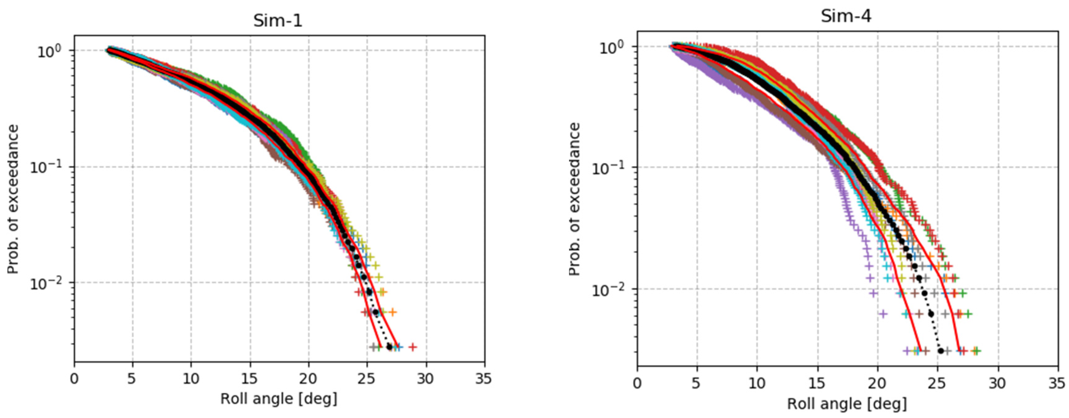
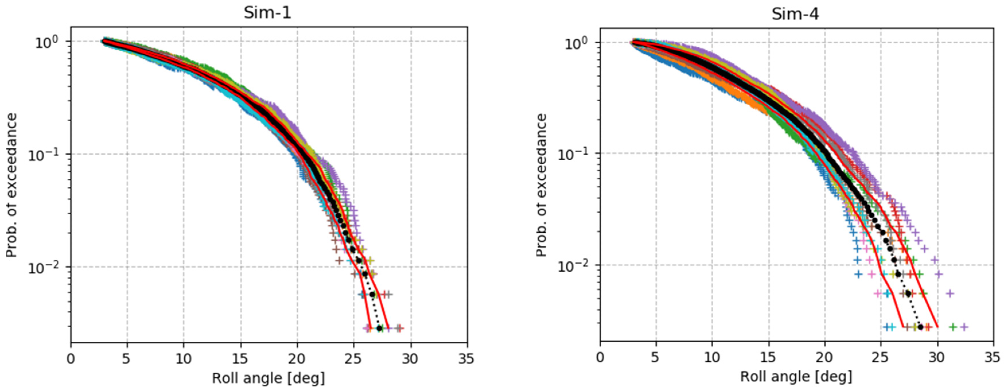
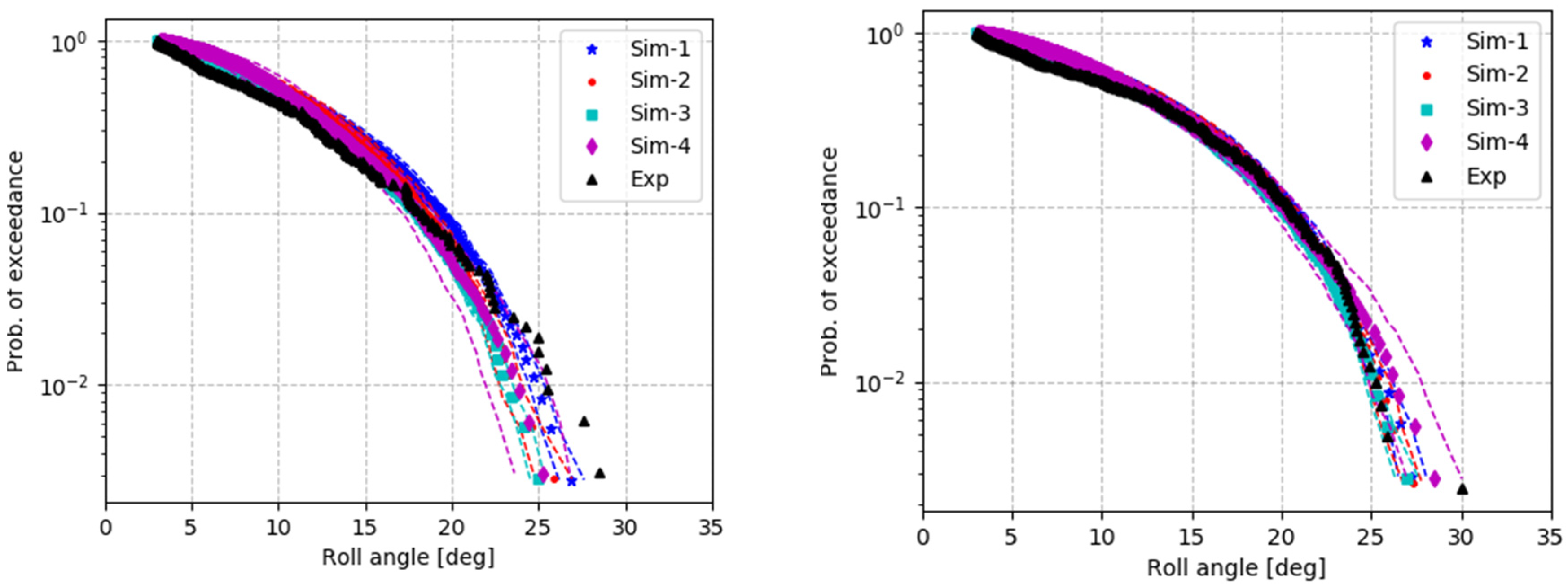
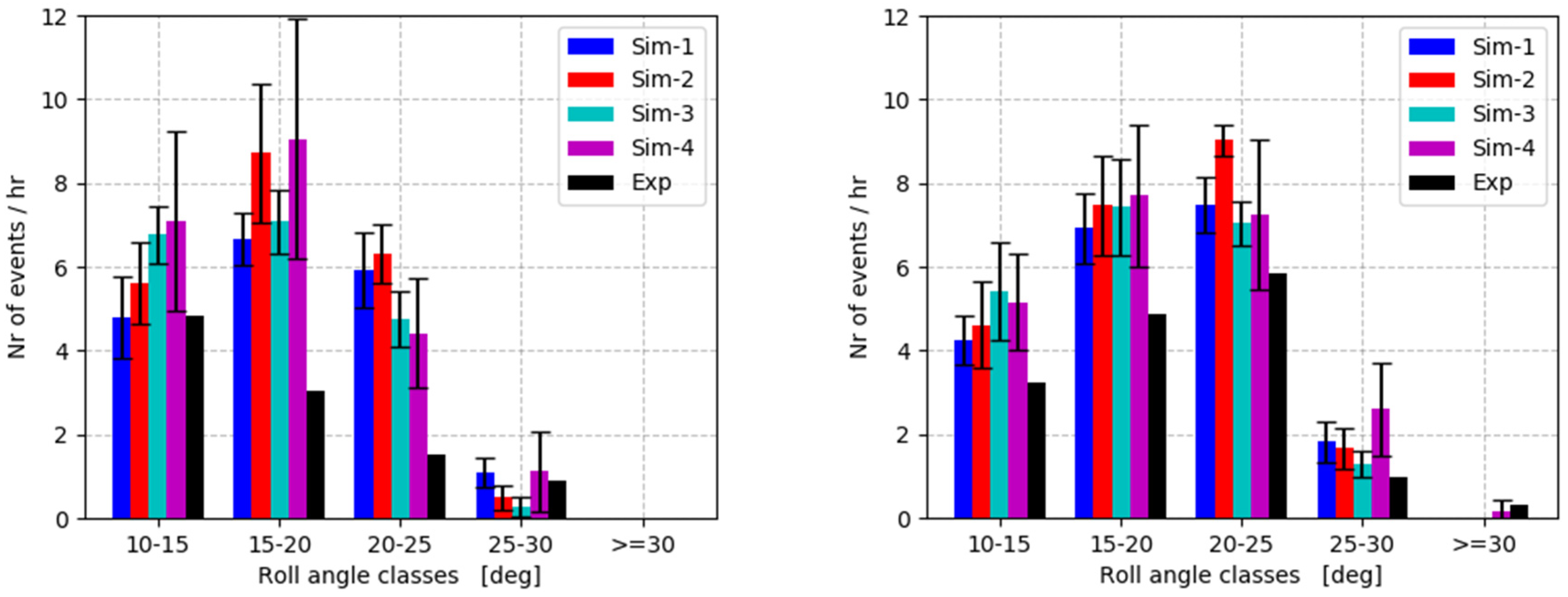
7.1. Probabilistic Analysis

The probability of exceedance of the extreme roll values, derived from the four simulation programs and from the experiment, is shown in Figure 7 for two sea states. Both the mean and the 95% confidence interval obtained from the simulations are shown. From the experiment, the result consists of one realisation of 3 h duration, as that is the only available data. The four programs produce generally similar results for both sea states, though there is some spread among them. The amount of spread is larger for the lower sea state, Hs = 7 m, than for the higher one, Hs = 8 m. For the lower sea state, three programs, Sim-2, Sim-3 and Sim-4, produce very similar mean values, while Sim-1 diverges from this group. The confidence intervals from the four programs vary, the one from Sim-4 being in general the widest. As for the higher sea state with Hs = 8 m, the four programs also produce similar mean values overall, although the mean from Sim-4 deviates from the others for the roll angles above 22°. The confidence intervals vary in their widths, with the one from Sim-4 being again the widest.

The variability in the extreme roll values was not determined in the experimental campaign. In that sense, the comparison of the numerical results to the experiments is incomplete. Considering the available data illustrated in Figure 7, it can be observed that the simulations produce non-conservative results for the extreme roll in the case of the lower sea state with Hs = 7 m. For the higher sea state, all the results of the simulations are conservative.

Figure 8 shows the number of parametric roll events per hour, divided into classes of roll angles from the four programs and the experiment for the two head sea cases. There is overall a reasonable agreement among the four programs, though the error bars of the 95% confidence interval are large in some cases. The simulations show a significantly larger number of events in the medium classes than the experiments. The number of events classified as parametric roll (φ > 30°) is very low, so no conclusions can be drawn on this. The typical distributions of the number of events in the experiments (a steadily decreasing number of events in the increasing classes for the 7-m sea state, and a large number of events in the 20°–25° class for the 8-m sea state) is much better reproduced by the simulations in the 8-m sea state than in the 7-m sea state. The distribution of events over the classes resulting from the simulations is quite similar for the two sea states.

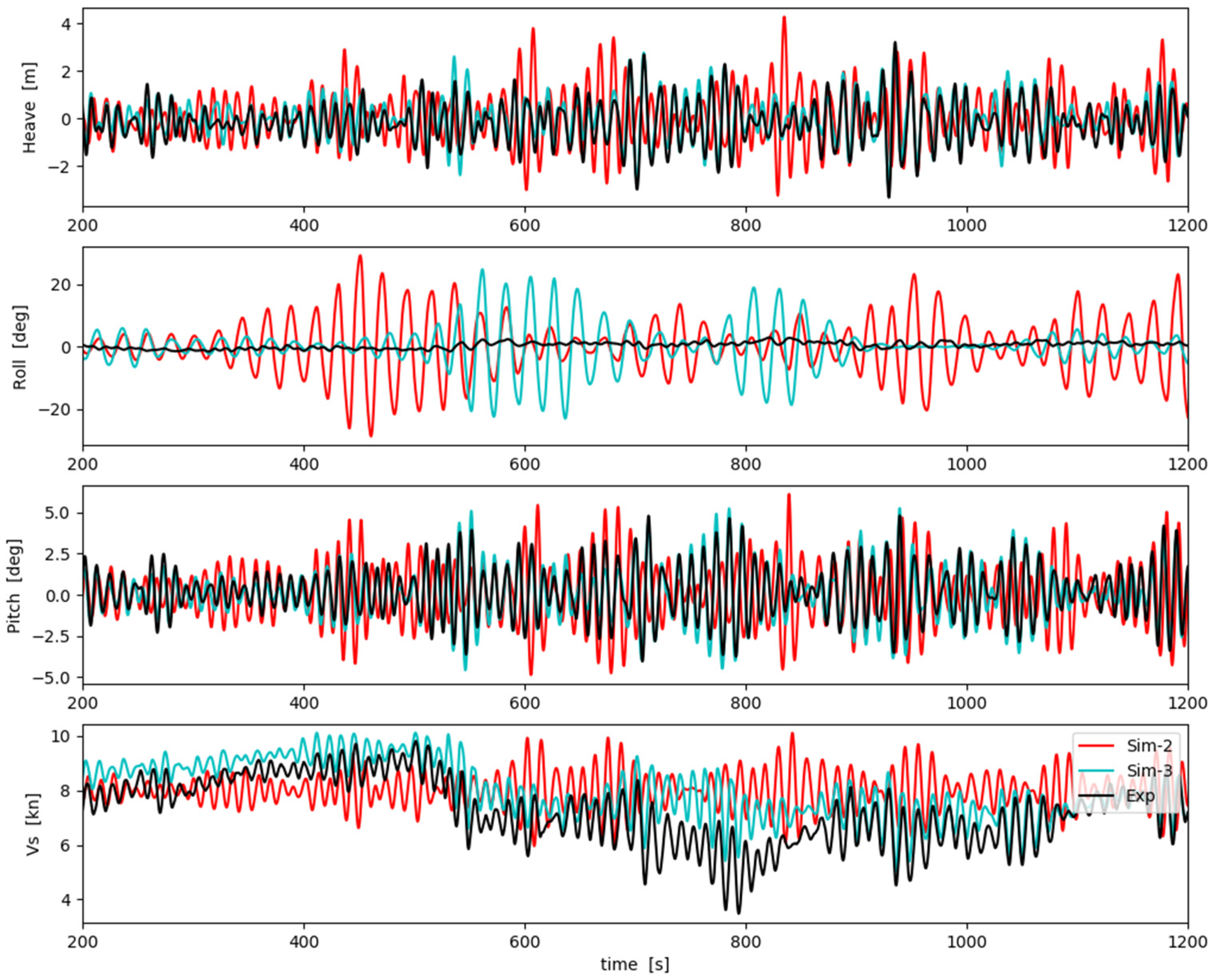
7.2. Deterministic Analysis

The first case selected for the deterministic analysis was a run in the Hs = 7 m sea state. This run was chosen because the roll motion is very low in the first part and there is a parametric roll event in the second part. The resulting time traces of two simulations and of the measured signals are shown in Figure 9. The figure shows that the heave and pitch motions are well predicted. The Sim-2 model predicts a parametric roll event resulting from the high wave group at around t = 300 s, while Sim-3 and the experiment do not produce an event at that instance. The large event predicted by Sim-2 could be a consequence of the start-up. Both simulation programs predict an important event in the interval 600 < t < 800 s; this event was not present in the experiments. The large event within 1000 < t < 1200 s is predicted accurately by both models, although the simulated events have a longer duration than the one in the experiment.

The second case was a run in the Hs = 8 m sea state. This run was chosen because the waves were high, but parametric roll did not occur. The simulation programs were proven to have the tendency to overpredict the occurrence of parametric roll; this was concluded before from the results in regular waves [3]. Figure 8 shows that the same is true in irregular waves.

The time traces of the simulations are compared to the measured signals in Figure 10. The results of both simulations indeed show several parametric roll events, although at different parts of the run. The measurements show no indication of parametric roll. The peaks in the heave and pitch motions resulting from the Sim-2 simulations are quite large, while those from the Sim-3 simulations correspond much better to the experimental values.

8. Comparison of Results in Following Seas

8.1. Probabilistic Analysis

The statistics of the extreme roll values from the four simulation programs and the experiment are shown in Figure 11. The mean and the 95% confidence interval from the simulations are also shown in this plot. The means of the exceedance probabilities from the four programs are similar for ϕ < 20°; after this value they split into two groups. The means estimated by Sim-1 and Sim-4 indicate lower probabilities than those by Sim-2 and Sim-3 for the roll angles larger than 20°. All four programs estimate lower probabilities than the measurement for the roll angles above 30°, considering the available measurement data. It is concluded that the simulation programs are non-conservative in this condition. This conclusion is supported by the bar diagram shown in Figure 11 (right); the number of events in the experiments is lower than those resulting from the simulations for all classes, except for the class φ > 30°.

8.2. Deterministic Analysis

Figure 12 shows the first case selected for deterministic comparison in the following seas. This run was chosen because there is an important parametric roll event in the second part of the run. The time traces of heave, roll, pitch and vessel speed from the experiment and two programs, Sim-2 and Sim-3, are illustrated in the figure. The agreement to the experiments is astonishing considering the results in the head seas. There is an important difference in the loading condition, and hence in the roll natural period, between the following and head sea cases. The natural roll period for the experiments in head seas was Tφ = 23.4 s, while for the experiments in following waves it was Tφ = 34.1 s (Table 1). It might be that at this lower encounter frequency of the waves at which parametric roll is initiated, the ratio of the diffraction force to the Froude–Krylov force is much lower, and that the modelling in the simulation programs (that ignore non-linear diffraction forces) is then closer to reality. This suggestion is detailed in Section 10.

The results of the second deterministic comparison in the following seas are shown in Figure 13. The duration is 1145 s. This run was chosen because it starts with low roll motions, and then a parametric roll event with a maximum roll motion of 33.5° develops. This event dies out, and about 500 s later a second event develops with a similar maximum roll value.

Time traces of heave, roll, pitch and vessel speed, from the experiment and two simulations programs, Sim-2 and Sim-3, are shown in Figure 13. Similar to the results in Figure 12, the agreement is much better than in head seas. Both parametric roll events are captured, and the peak roll values of the events are accurately predicted.

9. Discussion

9.1. Objective

The intention of this study was to compare existing simulation programs “as is”, and using settings according to the best practice of the owners of each of the programs. The background of this choice was that a ship operator could ask any of these companies to do these simulations, expecting similar results that are also close to experimental values.

Although the differences in the results of the four simulation programs are globally not large, the focus is on the probability of exceedance of a roll angle larger than 30°. Only an event with such a roll angle is classified as a parametric roll event. Looking at the results in this way, there are important differences in the four simulation programs. The order of the results of the programs, in the sense of the one predicting the largest probability for φ > 30° to the one predicting the lowest probability, is not the same for the three conditions.

It is acknowledged that the results of this study raise questions regarding the cause of the differences. An investigation into the cause of the differences was outside the scope of the present study, but it is the logical next step to take. Essentially, this next step consists of two phases: first, to find reasons for the differences between the simulation programs as they are now and to reduce them, and secondly to improve the accuracy of all the programs. The discussion presented here suggests possible improvements for this second phase.

9.2. Modelling the Waves

It is concluded from the results of this study that, although roll damping is a crucial effect, using the same roll damping model does not guarantee identical results when different simulation programs are being used. Apparently, other aspects are important as well. One of the candidate aspects is the model for the irregular seas. All programs use a linear combination of wave frequencies, but the number and the choice of values for the frequencies also play roles. A comparison in regular waves of these same programs, as done by Kapsenberg [3], showed important differences for the threshold wave amplitude, but the roll angle of parametric roll in 2.5- and 3.0-m wave amplitudes was similar. On the other hand, the deterministic comparison was made with a defined number of frequencies, amplitudes and phase angles. In that sense, the input was identical for programs Sim-2 and Sim-3. This identical input resulted in similar heave and pitch motions for the case of the 7-m sea state (Figure 9), but there were rather different results for those parameters in the case of the 8-m sea state (Figure 10).

9.3. Variation in the Stability

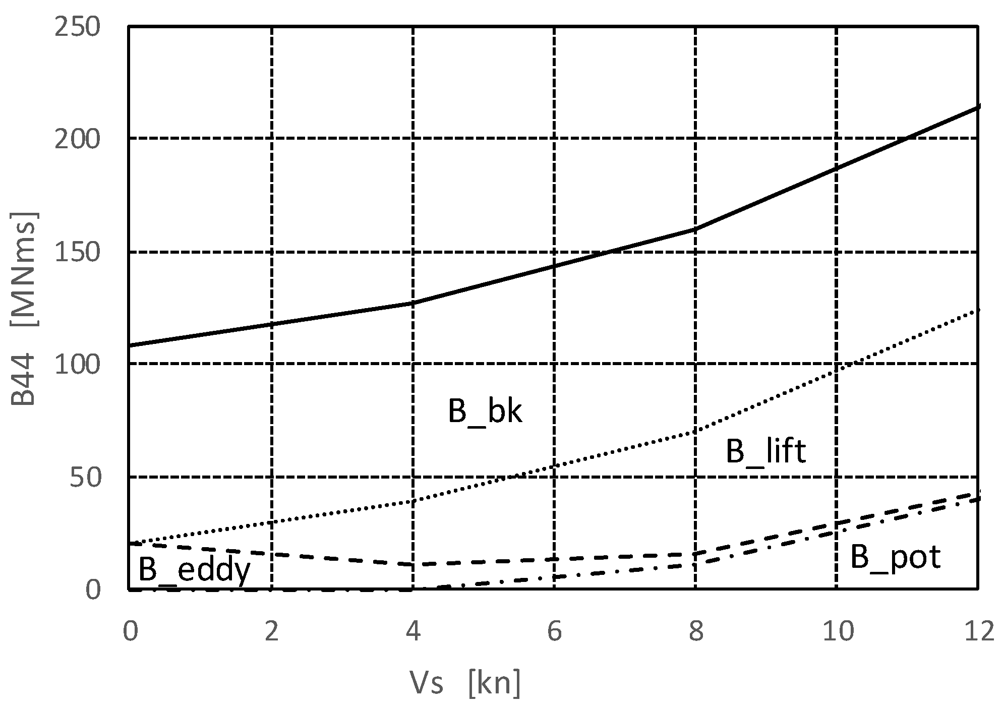
The physical explanation of parametric roll is classically based on roll stability variations when a vessel sails in waves (Paulling [26]). The time-dependent roll stability leads to the Mathieu equation, Equation (5), which is the simplest mathematical model for predicting the probability of parametric roll. The Mathieu equation is a linear differential equation, in which an oscillating restoring term with amplitude k∙m is added to the constant restoring coefficient k. The solution of the Mathieu equation can be illustrated in a figure, known as the Ince–Strutt diagram, Figure 14. This figure shows areas with stable (bounded) and unstable (unbounded) solutions that predict parametric roll events reasonably well.

$$\ddot{\phi }+k\left[1-m \cos \left(\omega t\right)\right]\phi =0$$

(5)

The time-dependent roll stability term is a necessary prerequisite in a mathematical model to predict parametric roll. Practical implementations of this effect in mathematical models are usually based on the calculation of the wave elevation along the hull for each time step. This calculation often uses the undisturbed wave and the motions of the ship to determine the wetted surface. The force is then determined by a pressure integration; the pressure above the calm water surface is determined by the hydrostatic component only, or by using Wheeler stretching [22] for the dynamic part. This non-linear restoring term is often accompanied by a non-linear roll damping term, but other components of the equations of motion are based on linear theories.

9.4. Roll Damping

The use of experimental values for the roll damping does not guarantee that all problems related to this parameter have been solved. An important part of the roll damping is due to the bilge keels. The potential flow damping is low, due to the long natural roll period. The roll damping contributions, as a function of the forward speed, are shown in Figure 15. The roll damping in this figure is based on Ikeda’s method. The calculation is essentially based on a forced motion in calm water, and as such the results are directly comparable to the roll decay and forced moment tests done in this campaign. In waves, the situation is different; the forces on the bilge keels are partly due to the velocities of the incoming and diffracted wave. This contribution is neglected in Ikeda’s method.

9.5. Relation between Parametric Roll Amplitude and Wave Height

The relation between the amplitude of the parametric roll angle and the wave height is very non-linear. First, there is a threshold wave height below which parametric roll does not occur. Secondly, it appears that the roll angle stabilises at some wave height, and does not further increase. These effects were also quite apparent in the results of the regular waves tests (see Kapsenberg et al.) [3].

It has been accepted [28] that the magnitude of the roll damping is largely responsible for the value of the threshold wave height. Therefore, it could be advisable to increase speed in order to increase the roll damping and hence to reduce the risk of parametric roll. The effect of forward speed was noted in the experiments in regular waves; tests at a speed of 10 kn did not show a tendency for parametric roll. If this statement is accepted, it should matter a lot if a second or a third order model is used to describe the damping, as shown in Figure 1 (the damping for φ = 0 is a factor different between these two models).

It is not clear why the roll motion stabilises at a certain wave height. There is a publication that suggest that the amplitude even decreases in very high waves; Hashimoto et al. [29] showed experimental results that indicated a decrease of the parametric roll angle for a wave steepness > 0.05. Since the wave-length of interest is in the order of the ship length, this is a wave with a height of more than 11 m, which is the order of the draft of the KCS. This is an extreme condition by all standards. A less extreme explanation might lie in the third order behaviour of the damping curve (Figure 1). A parametric roll excitation that increases linearly with the roll angle explains both the threshold wave amplitude and the stabilisation of the roll angle. This point will be developed in the next paragraph.

9.6. Nonlinear Diffraction

The non-linear effect of the incoming wave is accounted for by calculating the wetted surface of the hull at each time step. The Froude–Krylov force is then based on a pressure integration over the wetted hull. The presented simulation programs all include just the linear diffraction forces. It has been suggested by Dallinga [30] and Bu et al. [31] that the non-linear diffraction forces play a role in the occurrence of parametric roll events. Dallinga [30] used linear calculations on a heeled vessel to estimate non-linear diffraction effects. Bu et al. [31] used a more complicated (and more CPU-intensive) hydrodynamic model, a body-exact method, to calculate the hydrodynamic forces at each time instant using a new panelisation. They compared results of stability calculations in waves using the body-exact method to results of a linear program and a heeled vessel, similar to Dallinga. They found perfect agreement for small angles of heel (up to 12°) and some differences for large angles. Limited results were shown for parametric roll calculations; for one condition it appeared that the predicted roll amplitude was similar when comparing the two methods. The effect on the onset of parametric roll was not studied.

It is proposed here to use the approach of a linear diffraction program, and to approximate non-linear diffraction by using a heeled vessel in the input. Calculations were carried out for the KCS vessel in the LC-1 condition, at a speed of 8 kn, in head seas at three angles of heel (φ = 2.5°, 5.0° and 10°). The natural roll frequency for this condition is ω_φ = 0.266 rad/s. The condition that the wave-encounter period is twice the roll natural frequency corresponds to an earth fixed wave frequency ω₀ = 0.448 rad/s. Figure 16 (left) shows the results of the calculation at this frequency. The excitation and diffraction roll moments (F4) are split into a component in-phase with the roll motion, Re{F4}, and a component in-phase with the roll velocity, Im{F4}. There appears to be a significant effect on both components, whether including the diffraction force or not. For both components, it results in a significant reduction of the magnitude. The same figure has been made for the KCS in the LC-12 loading condition in following waves [Figure 16 (right)]. The natural roll frequency for this loading condition is ω_φ = 0.184 rad/s; this corresponds, in following waves and a speed Vs = 8 kn, to an earth fixed wave frequency ω₀ = 0.456 rad/s. Figure 16 (right) shows that the effect of adding the diffraction roll moment to the excitation is much smaller than for the head seas case.

Note that this frequency corresponds to a wave-length that is similar to the critical condition in head seas, the wave-length to ship-length ratio is 1.3.

Another observation that can be based on Figure 16 is that both moments, due to the incoming and the diffracted wave, are linear, with respect to the heel angle. This means that this moment (in head and following seas) can be modelled as:

$$F4=\phi F{4}_a\cos \left({\omega }_{e}t+{ϵ}_{F4}\right)$$

(6)

We assume that the roll motion φ is also oscillating as a harmonic function, with amplitude φ_a and frequency ω_φ. We define the phase angle of the roll as zero, so the phase angle in Equation (5) is relative to the roll motion. If we introduce this harmonic oscillation of the roll motion in Equation (5), we have:

$$F4=\frac{1}{2}{\phi }_{a}F{4}_a\left[\cos \left({\omega }_{e}t+{ϵ}_{F4}-{\omega }_{\phi }t\right)+\cos \left({\omega }_{e}t+{ϵ}_{F4}+{\omega }_{\phi }t\right)\right]$$

(7)

The classical condition for parametric roll is:

$${\omega }_e=2{\omega }_{\phi }$$

(8)

When this is substituted into Equation (6), we arrive at:

$$F4=\frac{1}{2}{\phi }_{a}F{4}_a\left[\cos \left({\omega }_{\phi }t+{ϵ}_{F4}\right)+\cos \left(3{\omega }_{\phi }t+{ϵ}_{F4}\right)\right]$$

(9)

This equation shows that a vessel sailing in waves with an encounter frequency of twice the roll natural frequency experiences an excitation in the roll natural frequency and in a frequency of three times the roll natural frequency. Both components contribute to the energy input of the vessel, which should be compensated for by the roll damping.

Similar to the derivation above, the expressions for the non-linear damping and the oscillating part of the restoring force also result in ${\omega }_{\phi }t$ and $3{\omega }_{\phi }t$ terms in the equation of motion. The ship will respond mainly on the ${\omega }_{\phi }$ terms; a force oscillating with three times the natural frequency does not provoke a significant response.

9.7. Effect of Water on Deck

Another component of nonlinear excitation may come from the water on the submerged deck. This topic has been investigated for a vessel at zero speed (FPSO) by Greco et al. [32]; they found that the water on deck had a limited effect on parametric roll. In this case, it has been found that water on the deck has a significant effect on extreme roll angles. There will of course be no effect on the onset of parametric roll. Once parametric roll occurs, and as the roll motion grows, the edge of the deck surface may be submerged, and the water on deck is detrimental to the stability of the vessel, and will increase the roll response. For the irregular following seas with Hs = 4 m, the simulated roll motions and a corresponding snapshot of a submerged deck edge are shown in Figure 17. A deck-in-water model, considering hydrostatic and Froude–Krylov pressures, is applied to the submerged deck surface. The figure shows that water on the deck increases the extreme roll angles larger than 30°. This result demonstrates the importance of accurate deck modelling in the numerical simulations, as well as in the model experiments, to determine the probability of parametric roll, as it is defined here.

10. Conclusions

This article presents results of a comparison study of different numerical simulation programs, and dedicated model experiments on the topic of parametric roll. The conditions for the experiments and simulations consisted of head and following seas in high and moderate sea states, respectively. The speed of the subject vessel, the Korean Container Ship KCS, was about 8 kn, which is a realistic speed considering the sea conditions.

It appeared that parametric roll occurred frequently, both in the simulations and in the experiments. Similar to an earlier similar comparison of the same vessel in regular waves, the simulations showed more parametric roll events than were measured during the experiments. This was in particular the case for events with medium extreme values in the head seas condition.

It cannot be concluded that these simulations are always conservative or always non-conservative. Sometimes they are conservative, sometimes they are not. A complicating factor is that the extreme roll motions in a 7-m sea state appear to be larger than those in an 8-m sea state (with the same period and at the same speed).

The differences between the various simulation programs are not very large, considering the extreme value distributions of the roll motions. However, if one considers the probability of a roll angle large enough to classify the event as parametric roll (roll angle > 30°), there are important differences. This is also illustrated by the bar diagrams giving the number of events in a certain roll angle range [Figure 8 and Figure 11 (right)].

For a validation study, one needs to compare converged statistical results. Convergence was shown for the simulations by considering 10 realisations of 3 h each. For the experiments, it could be shown that convergence was not achieved for 3-h experiments. To prove convergence, a series of experiments with different seeds is necessary, but a duration of 3 h might not be necessary.

The considered simulation programs do not model non-linear effects of the diffraction forces. It has been shown, by using a linear diffraction program for a heeled vessel, that the effect of the non-linear diffraction force is important (more so in head seas than in following seas). This suggests that a useful improvement of simulation programs can be made by adding this effect.

References

1. IMO. Report of the Drafting Group on Intact Stability, Finalization of Second Generation Intact Stability Criteria; IMO Document SDC 7/WP; IMO: London, UK, 2020. [Google Scholar]
2. IMO. Report of the Correspondence Group on Intact Stability, Finalization of Second Generation Intact Stability Criteria; IMO Document SDC 4/5/1/Add; IMO: London, UK, 2016. [Google Scholar]
3. Cooperative Research Ships. Available online: http://www.crships.org/web/show (accessed on 7 May 2020).
4. Kapsenberg, G.K.; Abeil, B.; Kim, S.; Wandji, C.; Ruth, E.; Pages, A. On parametric roll predictions. In Proceedings of the 17th International Ship Stability Workshop (STAB2019), Helsinki, Finland, 10–12 Jun 2019. [Google Scholar]
5. France, W.; Levadou, M.; Treakle, T.W.; Paulling, J.R.; Michel, R.K.; Moore, C. An investigation of head-sea parametric rolling and its influence on container lashing system. Mar. Technol. 2003, 40, 1–19. [Google Scholar]
6. Spanos, D.; Papanikolaou, A. Benchmark Study on Numerical Simulation Methods for the Prediction of Parametric Roll of Ships in Waves. In Proceedings of the 10th International Conference on Stab of Ships and Ocean Vehicles (STAB2009), St Petersburg, Russia, 22–26 June 2009. [Google Scholar]
7. Reed, A.M. 26th ITTC Parametric Roll Benchmark Study. In Proceedings of the 12th International Ship Stability Workshop (STAB2011), Washington, DC, USA, 12–15 June 2011. [Google Scholar]
8. Ikeda, Y.; Himeno, Y.; Tanaka, N. On Eddy Making Component of Roll Damping Force on Naked Hull; Report No. 00403; Un. of Osaka Pref., Dept. of Naval Arch.: Osaka, Japan, 1978. [Google Scholar]
9. Ikeda, Y.; Himeno, Y.; Tanaka, N. Components of Roll Damping of Ship at Forward Speed; Report No. 00404; Un. of Osaka Pref., Dept. of Naval Arch.: Osaka, Japan, 1978. [Google Scholar]
10. Ikeda, Y.; Himeno, Y.; Tanaka, N. On Roll Damping Force of Ship—Effect of Friction of Hull and Normal Force of Bilge Keels; Report No. 00401; Un. of Osaka Pref., Dept. of Naval Arch.: Osaka, Japan, 1978. [Google Scholar]
11. Ikeda, Y.; Himeno, Y.; Tanaka, N. A Prediction Method for Ship Roll Damping; Report No. 00405; Un. of Osaka Pref., Dept. of Naval Arch.: Osaka, Japan, 1978. [Google Scholar]
12. Ikeda, Y.; Komatsu, K. On roll Damping Force of Ship—Effect of Hull Surface Pressure Created by Bilge Keels; Report No. 00402; Un. of Osaka Pref., Dept. of Naval Arch.: Osaka, Japan, 1979. [Google Scholar]
13. Himeno, Y. Prediction of Ship Roll Damping—State of the Art; Report No. 239; Un. of Michigan, Dept. of Naval Arch. and Marine Eng.: Ann Arbor, MI, USA, 1978. [Google Scholar]
14. Hashimoto, H.; Omura, T.; Matsuda, A.; Yoneda, S.; Stern, F.; Tahara, Y. Some remarks on EFD and CFD for ship roll decay. In Proceedings of the 13th International Conference Stability of Ships and Ocean Vehicles (STAB2018), Kobe, Japan, 16–21 September 2018. [Google Scholar]
15. Yu, L.; Ma, N.; Hirakawa, Y.; Taguchi, K.; Akagi, K. Free running model experiment and numerical simulation on the occurrence and early detection of KCS parametric roll in head waves. In Proceedings of the 13th International Conference Stability of Ships and Ocean Vehicles (STAB2018), Kobe, Japan, 16–21 September 2018. [Google Scholar]
16. Yu, L.; Taguchi, K.; Kenta, A.; Ma, N.; Hirakawa, Y. Model experiments on the early detection and rudder stabilization of KCS parametric roll in head waves. J. Mar. Sci. Technol. 2018, 23, 141–163. [Google Scholar] [CrossRef]
17. Ruiz, M.T.; Villagomez, J.; Delefortrie, G.; Lataire, E.; Vantorre, M. Parametric Rolling in Regular Head Waves of the KRISO Container Ship: Numerical and Experimental Investigation in Shallow Water. In Proceedings of the 38th International Conference on Ocean, Offshore and Arctic Eng. (OMAE2019), Glasgow, UK, 9–14 June 2019. [Google Scholar]
18. Shin, Y.-S.; Belenky, V.L.; Paulling, J.R.; Weems, K.M.; Lin, W.M. Criteria for parametric roll of large containerships in longitudinal seas. In Proceedings of the SNAME Annual Meeting, Washington, DC, USA, 30 September 2004. [Google Scholar]
19. Neves, M.A.S.; Rodríguez, C.A. A non-linear mathematical model of higher order for strong parametric resonance of the roll motion of ships in waves. Mar. Syst. Ocean Technol. 2005, 1, 69–81. [Google Scholar] [CrossRef]
20. SIMMAN 2008 Workshop. Available online: http://www.simman2008.dk/KCS/container.html (accessed on 8 May 2020).
21. Hasselmann, K.; Barnett, T.P.; Bouws, E.; Carlson, H.; Cartwright, D.E.; Enke, K.; Ewing, J.A.; Gienapp, H.; Hasselmann, D.E.; Meerburg, A. Measurements of Wind-Wave Growth and Swell Decay during the Joint North Sea Wave Project (JONSWAP); Ergänzungsheft 8–12; Deutsches Hydrographisches Institut: Hamburg, Germany, 1973. [Google Scholar]
22. Wheeler, J.D. Method for calculating forces produced by irregular waves. J. Pet. Technol. 1970, 22, 359–367. [Google Scholar] [CrossRef]
23. Lewandowski, E.M. Comparison of Some Analysis Methods for Ship Roll Decay Data. In Proceedings of the 12th International Ship Stability Workshop (STAB2011), Washington, DC, USA, 12–15 June 2011. [Google Scholar]
24. Wandji, C. Review of Probabilistic Methods for Dynamic Stability of Ships in Rough Seas. In Proceedings of the 17th International Ship Stability Workshop (STAB2019), Helsinki, Finland, 10–12 June 2019; pp. 47–56. [Google Scholar]
25. van Walree, F.; de Jong, P. Deterministic validation of a time domain panel code for parametric roll. In Proceedings of the 12th International Ship Stability Workshop (STAB2011), Washington, DC, USA, 12–15 June 2011. [Google Scholar]
26. Paulling, J.R. The transverse stability of a ship in a longitudinal seaway. J. Ship Res. 1961, 4, 37–49. [Google Scholar]
27. Butikov, E.I. Analytical expressions for stability regions in the Ince–Strutt diagram of Mathieu equation. Am. J. Phys. 2018, 86, 257–267. [Google Scholar] [CrossRef] [Green Version]
28. Francescutto, A.; Bulian, G. Nonlinear and stochastic aspects of parametric rolling modelling. In Proceedings of the 6th International Ship Stability Workshop, Glenn Cove, NY, USA, 13–16 October 2002. [Google Scholar]
29. Hashimoto, H.; Umeda, N.; Matsuda, A.; Nakamura, S. Experimental and Numerical Studies on Parametric Roll of a Post-Panamax Container Ship in Irregular Waves. In Proceedings of the 9th International Conference on Stability of Ships and Ocean Vehicles, Rio de Janeiro, Brazil, 25–29 September 2006. [Google Scholar]
30. Dallinga, R.P. Predicting Parametric Roll, SWZ|Maritime, 135, July–August 2014; pp. 44–47. Available online: https://www.swzmaritime.nl/pdf-archive/2014-edition-8/(accessed on 15 May 2020).
31. Bu, S.-X.; Gu, M.; Lu, J.; Abdel-Maksoud, M. Effects of radiation and diffraction forces on the prediction of parametric roll. Ocean Eng. 2019, 175, 262–272. [Google Scholar] [CrossRef]
32. Greco, M.; Lugni, C.; Colicchio, G.; Faltinsen, O.M. Numerical Study of Bilge-Keel Effect on Parametric Roll and Water on Deck for an FPSO. In Proceedings of the 34th International Conference on Ocean, Offshore and Arctic Eng. (OMAE2015), St. John’s, NL, Canada, 31 May–5 June 2015. [Google Scholar]
Figure 1. Roll damping for LC-1 at ωφ = 0.273 rad/s and vs. = 8 kn. Results of forced roll tests (full triangles) and of roll decay tests (other symbols). The best-fit quadratic model is displayed as a dashed red line, a cubic model is displayed as a blue dashed line.
Jmse 08 00474 g001
Figure 2. Visualisation of the analysis procedure of parametric roll events: plot of the roll motion (red line) and the envelope (blue lines), with the peak of each event in the interval defined by Equation (4), (black symbols).
Jmse 08 00474 g002
Figure 3. Ensemble statistics of the number of parametric roll events classified in different groups on the basis of the maximum roll angle in each event. The plot shows successive results 3 h, 6 h, 9 h, etc of simulations, with a maximum of 60 h. Sea state: Hs = 7 m, Tp = 13.5 s, speed Vs = 7.6 kn.
Jmse 08 00474 g003
Figure 4. Extreme value distributions of the roll motions from programs Sim-1 (left) and Sim-4 (right) for 10 realisations of the wave. Simulations were run in head seas with Hs = 7 m, Tp = 13.5 s and average speed Vs = 7.9 kn.
Jmse 08 00474 g004
Figure 5. Extreme value distributions of the roll motions from programs Sim-1 (left) and Sim-4 (right) for 10 realisations of the wave. Simulations were run in following seas with Hs = 4 m, Tp = 13.5 s and average speedVs = 7.9 kn.
Jmse 08 00474 g005
Figure 6. Results of the experiments in three sea states; two head waves (HW) and one following wave (FW), all at a speed of about 8 kn. One realisation of the wave with a duration of 3 h was run in the experiments. Left: probability of exceedance of extreme values of the roll motions. Right: number of parametric roll events per hour divided in classes of roll angles.
Jmse 08 00474 g006
Figure 7. Extreme value distributions of the roll motions from the four programs and experiment. The mean (markers) and the 95% confidence interval (dashed lines) obtained from 10 realisations of the wave are shown for the simulations. Durations of the experiment and each realisation in the simulations are 3 h. Left: Head waves, Hs = 7 m, Tp = 13.5 s, speed vs. = 7.6 kn. Right: Head waves, Hs = 8 m, Tp = 13.5 s, speed vs. = 7.9 kn.
Jmse 08 00474 g007
Figure 8. The number of parametric roll events per hour divided in classes of roll angles. Results of four sets of simulations, each the total of 10 simulations of 3 h duration, compared to results of experiments (3 h). The bars indicate the means and the error bars indicate the 95% confidence intervals obtained from 10 realizations for each simulation program. Left: Head sea with Hs = 7 m, Tp = 13.5 s, speed Vs = 7.6 kn, Right: Head sea with Hs = 8 m, Tp = 13.5 s, speed Vs = 7.9 kn.
Jmse 08 00474 g008
Figure 9. Results of deterministic comparison of a parametric roll event in irregular head seas (Jonswap spectrum, Hs = 7.0 m, Tp = 13.5 s, γ = 3.3), Vs ≈ 8 kn. Heave, roll, pitch and vessel speed from two programs, Sim-2 and Sim-3, are compared to the measurement.
Jmse 08 00474 g009
Figure 10. Results of deterministic comparison of a parametric roll event in irregular head seas (Jonswap spectrum, Hs = 8.0 m, Tp = 13.5 s, γ = 3.3), vs. ≈ 8 kn.
Jmse 08 00474 g010
Figure 11. Statistics of extreme values of the roll motions (left) and the number of parametric roll events/hour subdivided in classes (right). Results of 4 sets of simulations, each the total of 10 simulations of 3 h duration, compared to results of experiments (duration 3 h). The mean (markers) and the 95% confidence interval (dashed lines) obtained from 10 realizations of the wave are shown for the simulations (left). The mean (bars) and the 95% confidence intervals (error bars) obtained from 10 realizations are plotted on the right. Sea state: Following seas, Hs = 4 m, Tp = 13.5 s, speed vs. = 7.9 kn.
Jmse 08 00474 g011
Figure 12. Results of a first case of a deterministic comparison of a parametric roll event in irregular following seas (Jonswap spectrum, Hs = 4.0 m, Tp = 13.5 s, γ = 3.3), vs. ≈ 8 kn. Heave, roll, pitch and vessel speed calculated by Sim-2 and Sim-3 are compared to the measurement.
Jmse 08 00474 g012
Figure 13. Results of the second case of a deterministic comparison of a parametric roll event in irregular following seas (Jonswap spectrum, Hs = 4.0 m, Tp = 13.5 s, γ = 3.3), vs. ≈ 8 kn.
Jmse 08 00474 g013
Figure 14. Results of the Mathieu equation, the Ince–Strutt diagram. The figure shows stable (white) and unstable (shaded) regions, depending on restoring term k and amplitude of the stability variation m. (Figure reproduced from Butikov [27]).
Jmse 08 00474 g014
Figure 15. Roll damping contributions for the KCS, LC-1, at the natural roll period (Tφ = 23.4 s) as a function of the forward speed. The figure shows the contribution of different components: Potential flow component including the effect of forward speed, the eddy damping component, the lift component and the bilge keel component. For Vs = 8 kn, the bilge keels provide 56% of the total roll damping.
Jmse 08 00474 g015
Figure 16. Roll moment due to incoming wave only, and due to incoming + diffracted wave as a function of the initial heel angle. The moment has been split into two components; one component in-phase with the roll motion, Re{F4}, and the other component in-phase with the roll velocity, Im{F4}. Left: Results are for KCS, LC-1, ω0 = 0.45 rad/s, Hd = 180° and Vs = 8 kn; Right: KCS, LC-12, ω0 = 0.45 rad/s, Hd = 0° and Vs = 8 kn.
Jmse 08 00474 g016
Figure 17. Snapshot from a simulated maximum roll angle with water on the deck (left). Probability of exceedance for the values of the positive roll peaks with water on deck in the simulation (WoD) or no water on deck (No WoD) is shown together with the experimental result. The plot is based on 10 realisations of 3 h durations each, condition: following waves, Hs = 4 m, Tp = 13.5 s, Vs ≈ 8 kn.
Jmse 08 00474 g017