Artificial Structures Steer Morphological Development of Salt Marshes: A Model Study

 ,
, 

Abstract
1. Introduction
2. Materials and Methods
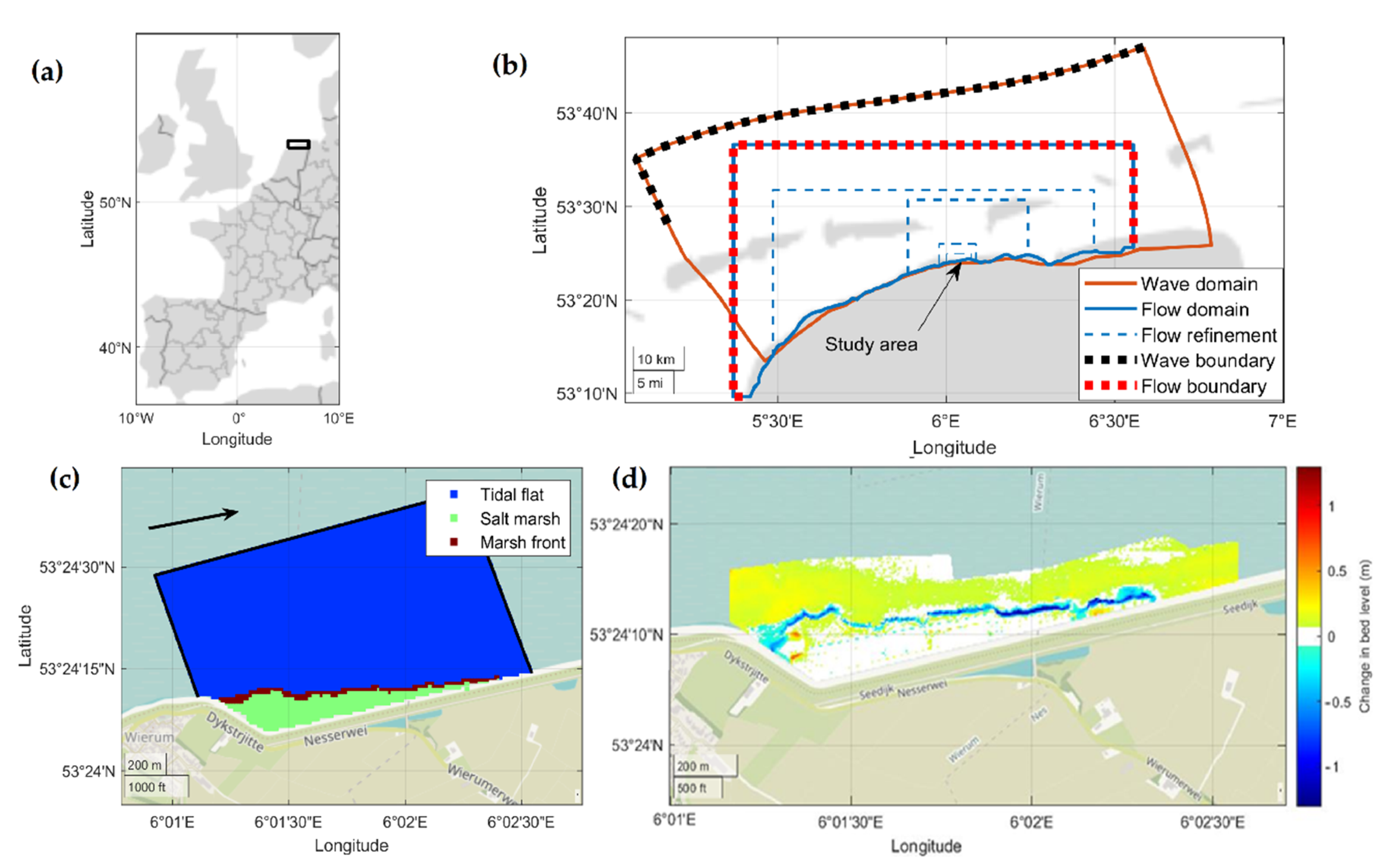
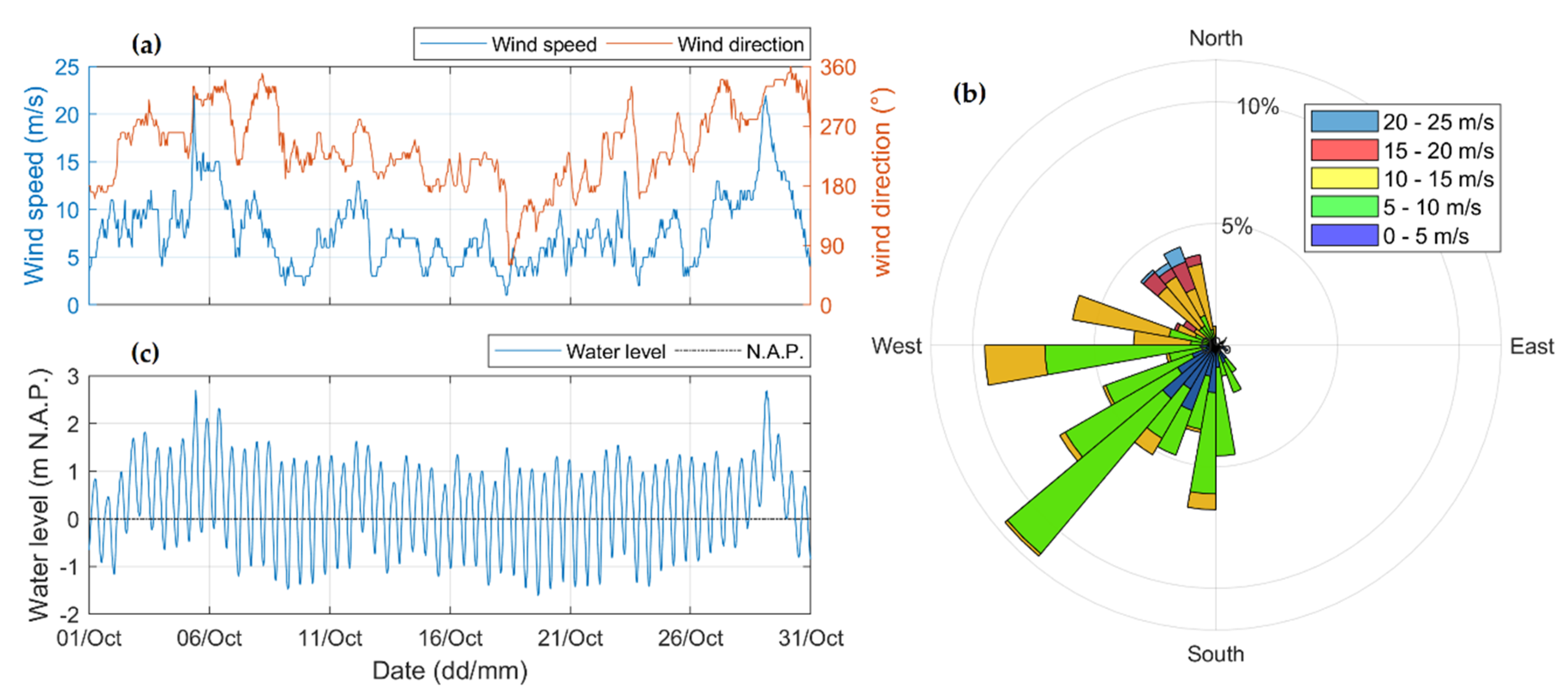
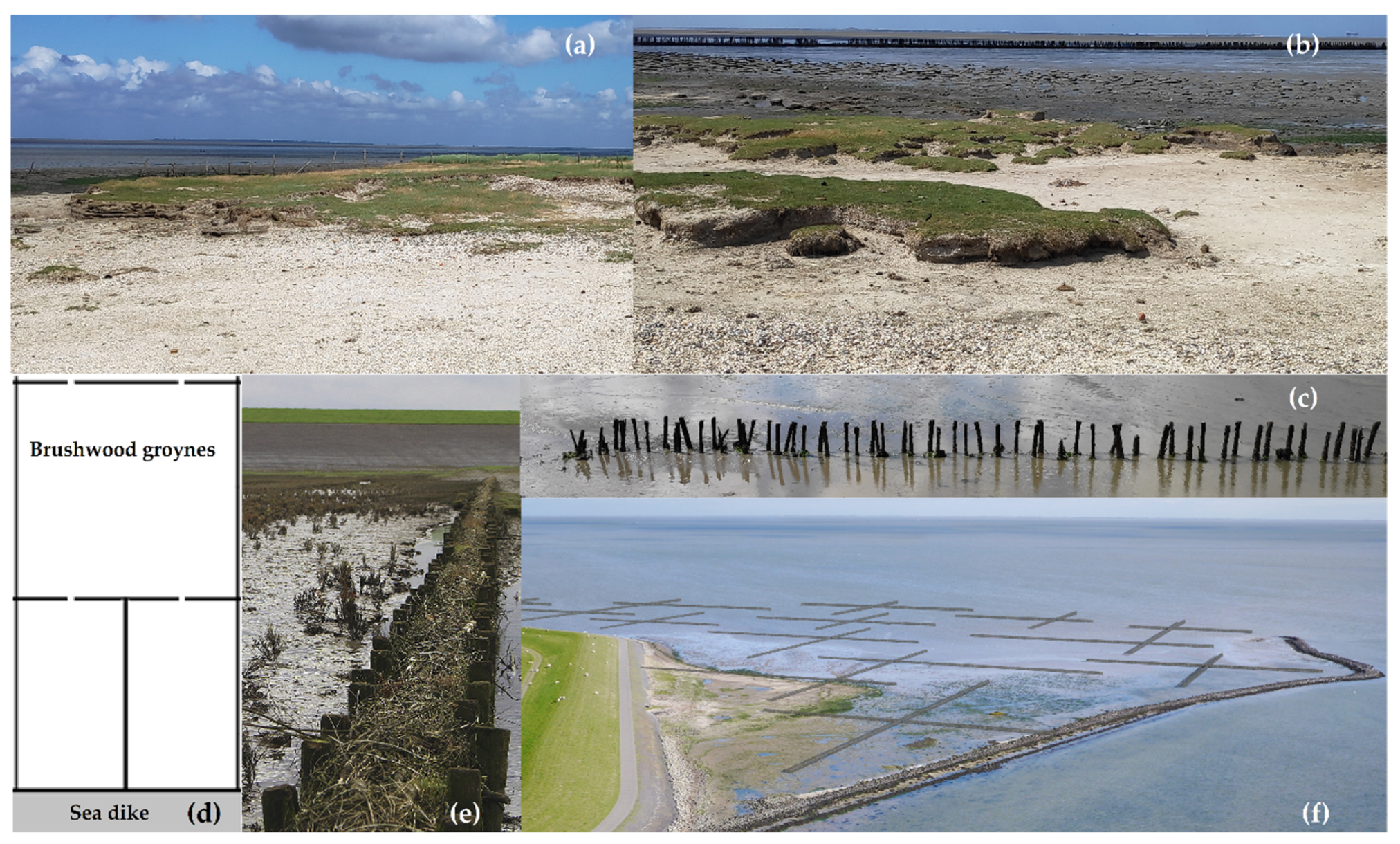
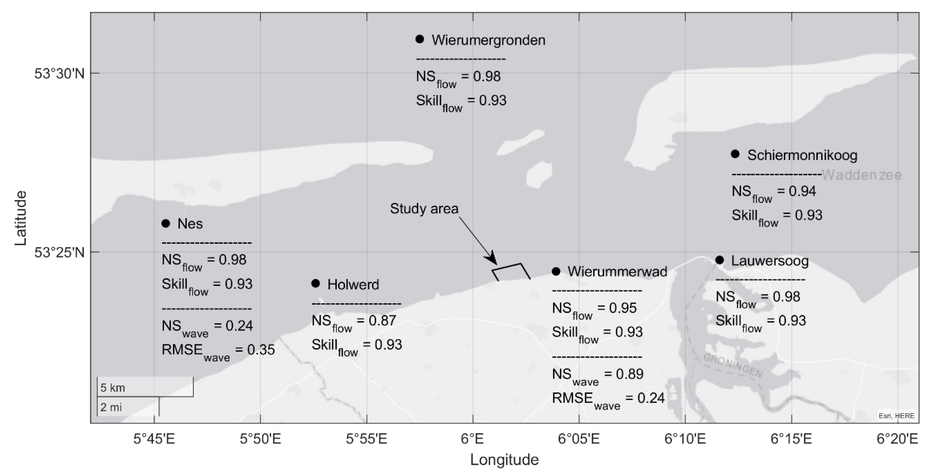
2.1. Study Area and Field Observations
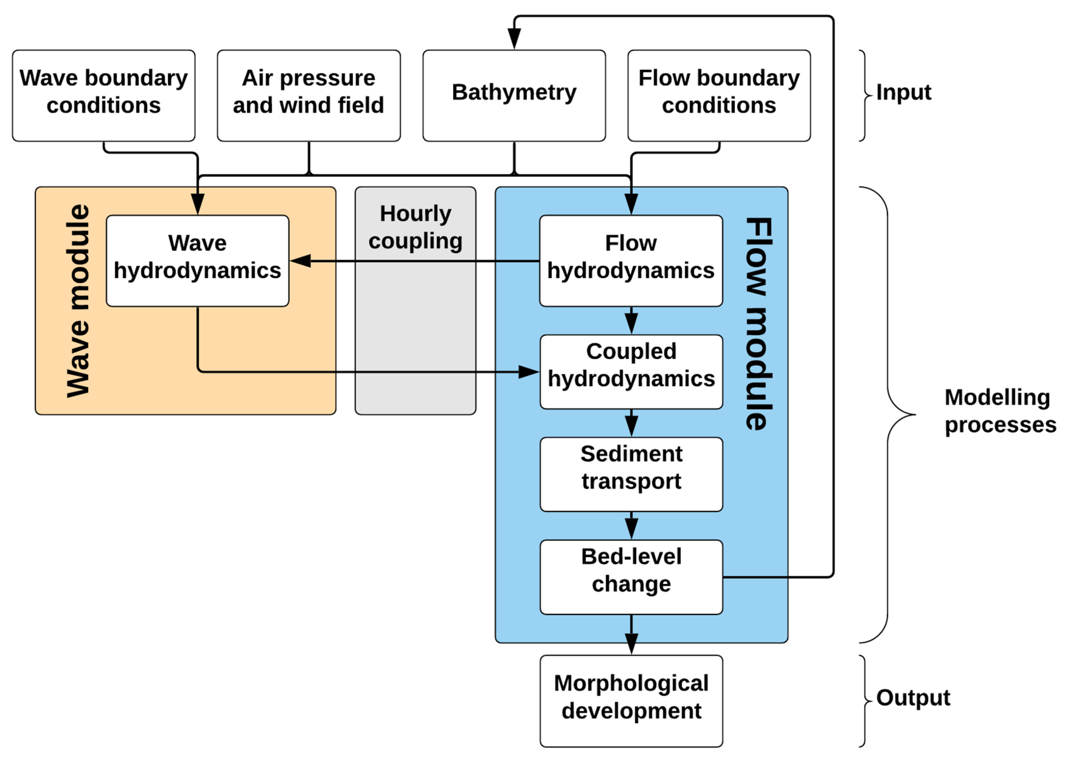
2.2. Delft3D Flexible Mesh Description
2.3. Addition of Artificial Structures
3. Results
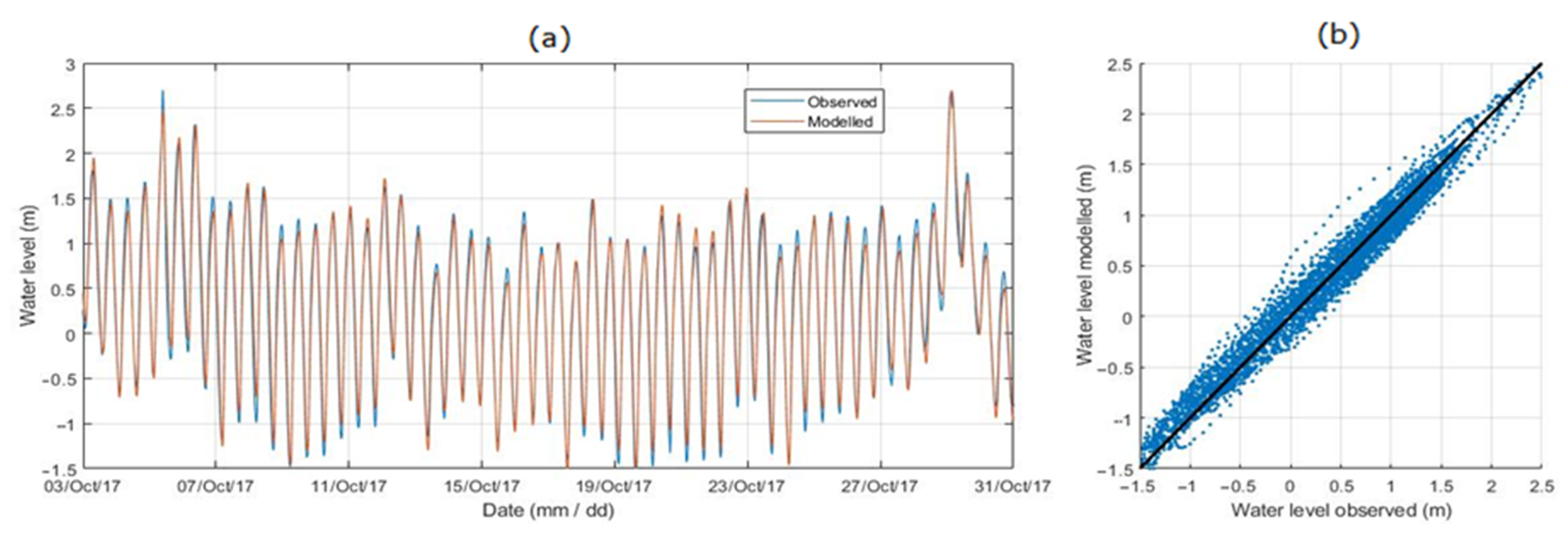
3.1. Hydrodynamics
3.2. Morphodynamics
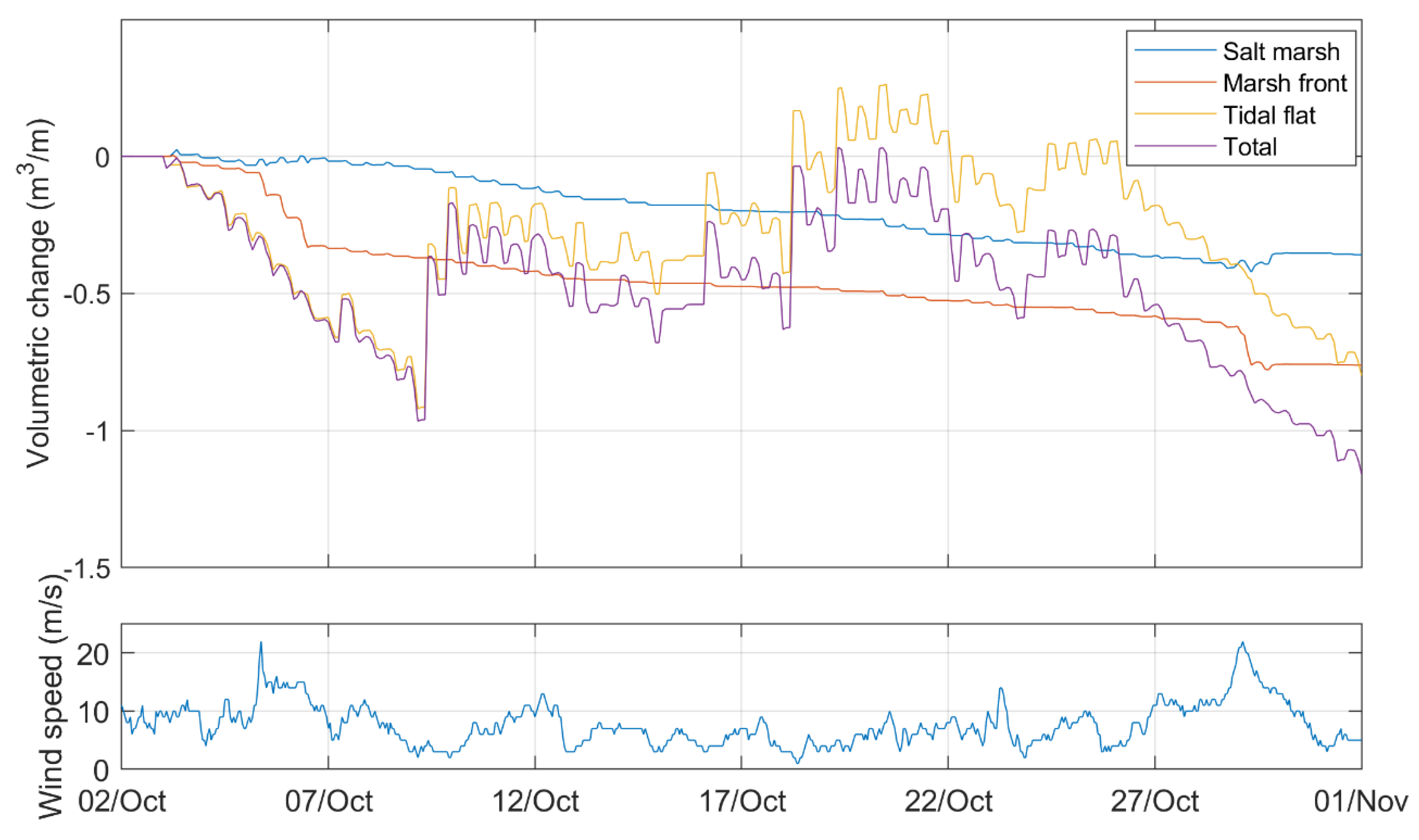
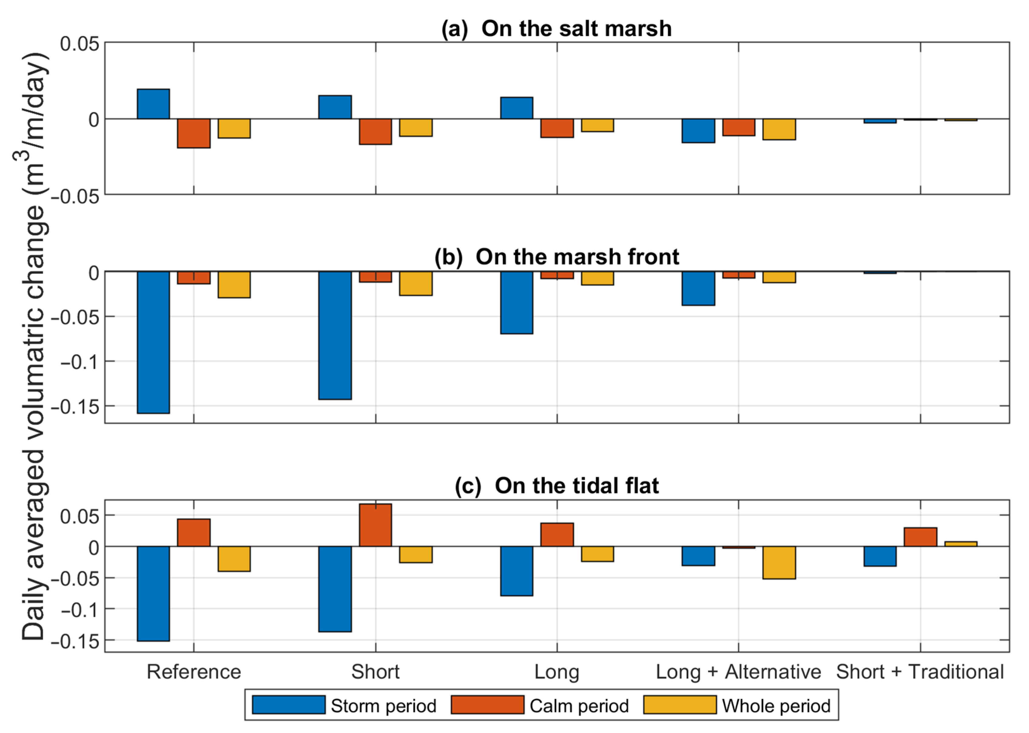
3.2.1. Salt Marsh Development without Human Interference
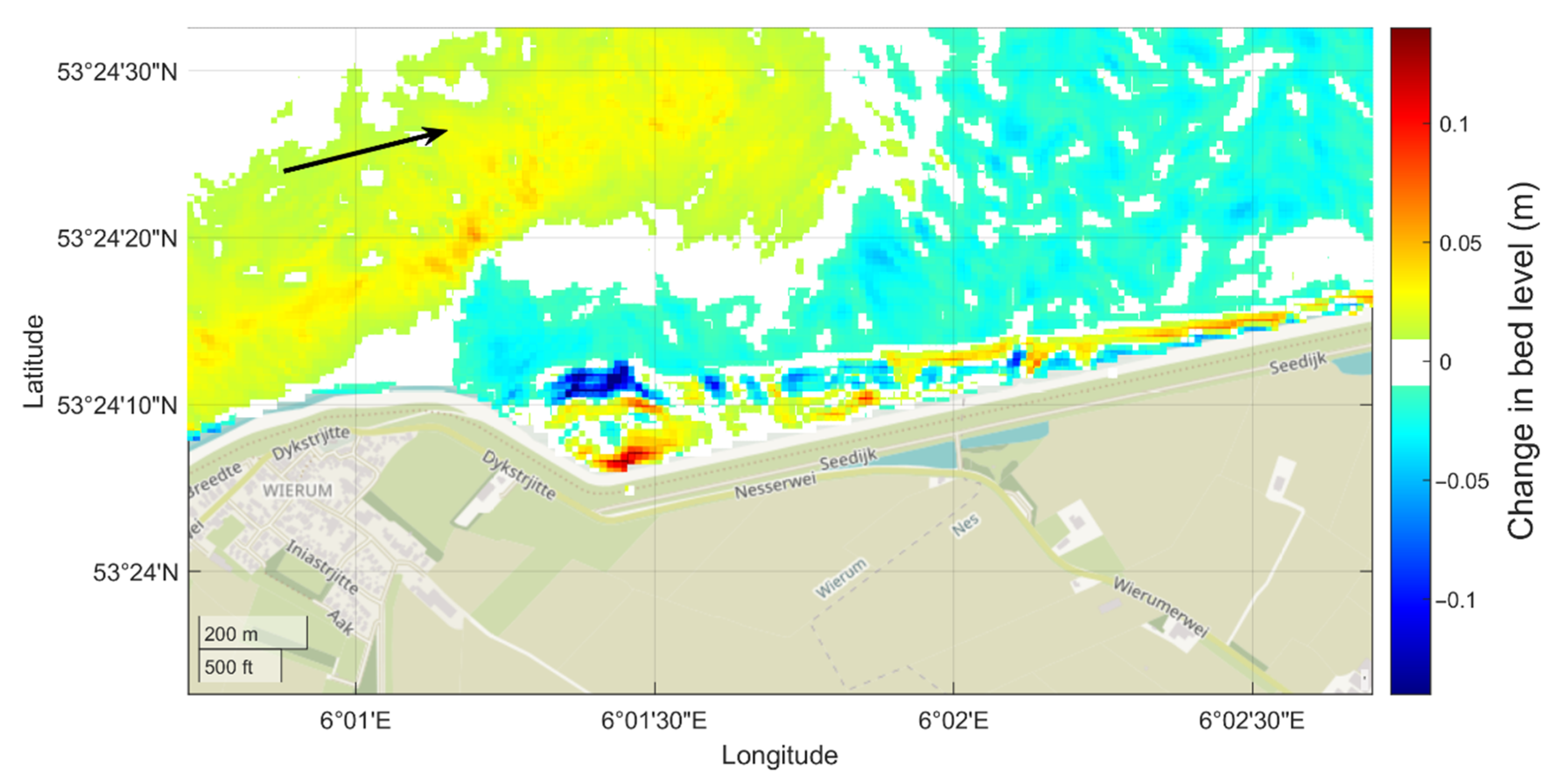
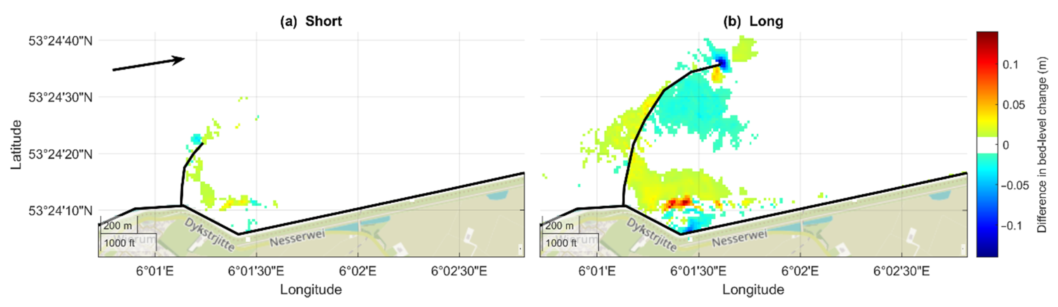
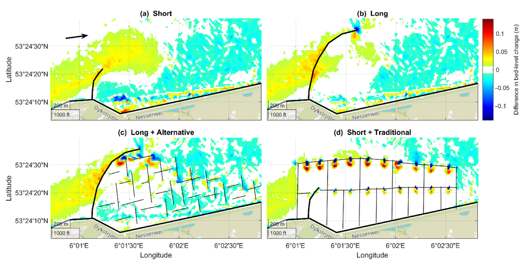
3.2.2. Impact of Artificial Structures
4. Discussion
4.1. Assumptions and Uncertainties
4.2. Default Simulation
4.3. Artificial Structures
4.4. General Applicability
5. Conclusions
Author Contributions
Funding
Acknowledgments
Conflicts of Interest
Appendix A. Model Setup
Appendix A.1. Domain and Timeframe

| Parameter | Value | Definition | Source |
|---|---|---|---|
| Domain and time frame | |||
| 0.021 | Manning coefficient | [45] | |
| 0.04 | Manning coefficient on the salt marsh | [46] | |
| 0.058 | Jonswap bed friction coefficient | i | |
| 0.15 | Smagorinsky factor | [48] | |
| 1 | Horizontal eddy diffusivity | [47] | |
| 0.7 | Maximum courant number | [32] | |
| Sediment dynamics | |||
| 2650 | Specific sediment density | [32] | |
| 1600 | Dry bed density | [32] | |
| 180 | Median grain size | ii | |
| 0.15 (-) | Mud fraction | ii | |
| 1.25 (-) | Calibration factor for wave-related bed-form roughness | ii | |
Appendix A.2. Hydrodynamics
Appendix A.3. Sediment Dynamics
Appendix B. Input Parameters Structure Implementation
| Parameter | Value | Definition | Module | Source |
|---|---|---|---|---|
| Short; Long | ||||
| 2.5 m | Height structure | Flow | i | |
| 2.5 m | Dam height | Wave | i | |
| 2.6 (-) | Alpha of dam | Wave | [32] | |
| 0.15 (-) | Beta of dam | Wave | [32] | |
| Long + Alternative | ||||
| Max 0.75 m above bed level -or- 1.45 m N.A.P. | Height structure | Flow | [33] | |
| 0.55 (-) | Transmission coefficient of brushwood groyne | Wave | [17] | |
| Short + Traditional | ||||
| Max 0.75 m above bed level -or- 1.45 m N.A.P. | Height structure | Flow | [33] | |
| 1.8 (-) | Alpha of brushwood groyne | Wave | [32] | |
| 0.10 (-) | Beta of brushwood groyne | Wave | [32] | |
Appendix C. Comparison Hydrodynamics
Appendix C.1. Flow Module

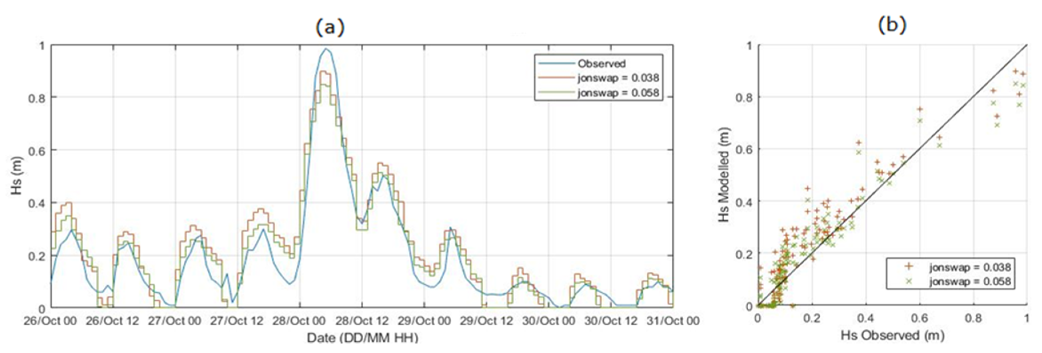
Appendix C.2. Wave Module

References
- Vuik, V.; Jonkman, S.N.; Borsje, B.W.; Suzuki, T. Nature-based flood protection: The efficiency of vegetated foreshores for reducing wave loads on coastal dikes. Coast. Eng. 2016, 116, 42–56. [Google Scholar] [CrossRef]
- Willemsen, P.W.J.M.; Borsje, B.W.; Hulscher, S.J.M.H.; van der Wal, D.; Zhu, Z.; Oteman, B.; Evans, B.; Moller, I.; Bouma, T.J. Quantifying Bed Level Change at the Transition of Tidal Flat and Salt Marsh: Can We Understand the Lateral Location of the Marsh Edge? J. Geophys. Res. Earth Surf. 2018, 123, 2509–2524. [Google Scholar] [CrossRef]
- Kirwan, M.L.; Temmerman, S.; Skeehan, E.E.; Guntenspergen, G.R.; Fagherazzi, S. Overestimation of marsh vulnerability to sea level rise. Nat. Clim. Chang. 2016, 6, 253–260. [Google Scholar] [CrossRef]
- Vuik, V.; Borsje, B.W.; Willemsen, P.W.; Jonkman, S.N. Salt marshes for flood risk reduction: Quantifying long-term effectiveness and life-cycle costs. Ocean Coast. Manag. 2019, 171, 96–110. [Google Scholar] [CrossRef]
- Wanner, A.; Suchrow, S.; Kiehl, K.; Meyer, W.; Pohlmann, N.; Stock, M.; Jensen, K. Scale matters: Impact of management regime on plant species richness and vegetation type diversity in Wadden Sea salt marshes. Agric. Ecosyst. Environ. 2014, 182, 69–79. [Google Scholar] [CrossRef]
- Chmura, G.L.; Anisfeld, S.C.; Cahoon, D.R.; Lynch, J.C. Global carbon sequestration in tidal, saline wetland soils. Glob. Biogeochem. Cycles 2003, 17. [Google Scholar] [CrossRef]
- Jones, M.B.; Donnelly, A. Carbon sequestration in temperate grassland ecosystems and the influence of management, climate and elevated CO2. New Phytol. 2004, 164, 423–439. [Google Scholar] [CrossRef]
- Costanza, R.; d’Arge, R.; De Groot, R.; Farber, S.; Grasso, M.; Hannon, B.; Limburg, K.; Naeem, S.; O’neill, R.V.; Paruelo, J.; et al. The value of the world’s ecosystem services and natural capital. Nature 1997, 387, 253–260. [Google Scholar] [CrossRef]
- Millard, K.; Redden, A.M.; Webster, T.; Stewart, H. Use of GIS and high resolution LiDAR in salt marsh restoration site suitability assessments in the upper Bay of Fundy, Canada. Wetl. Ecol. Manag. 2013, 21, 243–262. [Google Scholar] [CrossRef]
- Chang, E.R.; Veeneklaas, R.M.; Bakker, J.P.; Daniels, P.; Esselink, P. What factors determined restoration success of a salt marsh ten years after de-embankment? Appl. Veg. Sci. 2016, 19, 66–77. [Google Scholar] [CrossRef]
- Leonardi, N.; Ganju, N.K.; Fagherazzi, S. A linear relationship between wave power and erosion determines salt-marsh resilience to violent storms and hurricanes. Proc. Natl. Acad. Sci. 2016, 113, 64–68. [Google Scholar] [CrossRef] [PubMed]
- Bouma, T.J.; Van Belzen, J.; Balke, T.; Van Dalen, J.; Klaassen, P.; Hartog, A.M.; Callaghan, D.P.; Hu, Z.; Stive, M.J.; Temmerman, S.; et al. Short-term mudflat dynamics drive long-term cyclic salt marsh dynamics. Limnol. Oceanogr. 2016, 61, 2261–2275. [Google Scholar] [CrossRef]
- Hu, Z.; van Belzen, J.; van der Wal, D.; Balke, T.; Wang, Z.B.; Stive, M.; Bouma, T.J. Windows of opportunity for salt marsh vegetation establishment on bare tidal flats: The importance of temporal and spatial variability in hydrodynamic forcing. J. Geophys. Res. Biogeosci. 2015, 120, 1450–1469. [Google Scholar] [CrossRef]
- Silinski, A.; Fransen, E.; Bouma, T.J.; Meire, P.; Temmerman, S. Unravelling the controls of lateral expansion and elevation change of pioneer tidal marshes. Geomorphology 2016, 274, 106–115. [Google Scholar] [CrossRef]
- Poppema, D.W.; Willemsen, P.W.; de Vries, M.B.; Zhu, Z.; Borsje, B.W.; Hulscher, S.J. Experiment-supported modelling of salt marsh establishment. Ocean Coast. Manag. 2019, 168, 238–250. [Google Scholar] [CrossRef]
- Van Loon-Steensma, J.M.; Slim, P.A. The impact of erosion protection by stone dams on salt-marsh vegetation on two Wadden Sea barrier islands. J. Coast. Res. 2012, 29, 783–796. [Google Scholar] [CrossRef]
- Dao, T.; Stive, M.J.; Hofland, B.; Mai, T. Wave Damping due to Wooden Fences along Mangrove Coasts. J. Coast. Res. 2018, 34, 1317–1327. [Google Scholar]
- Vona, I.; Gray, M.W.; Nardin, W. The Impact of Submerged Breakwaters on Sediment Distribution along Marsh Boundaries. Water 2020, 12, 1016. [Google Scholar] [CrossRef]
- Schuerch, M.; Spencer, T.; Evans, B. Coupling between tidal mudflats and salt marshes affects marsh morphology. Mar. Geol. 2019, 412, 95–106. [Google Scholar] [CrossRef]
- Best, U.S.N.; van der Wegen, M.; Dijkstra, J.; Willemsen, P.W.J.M.; Borsje, B.W.; Roelvink, D.J.A. Do salt marshes survive sea level rise? Modelling wave action, morphodynamics and vegetation dynamics. Environ. Model. Softw. 2018, 109, 152–166. [Google Scholar] [CrossRef]
- Loon-Steensma, J.M.; Groot, A.V.; Duin, W.E.; Wesenbeeck, B.K.; Smale, A.J. Zoekkaart Kwelders en Waterveiligheid Waddengebied; Alterra-rapport 2391; Alterra: Wageningen, The Netherlands, 2012. [Google Scholar]
- RWS (Ed.) Actueel Hoogtebestand Nederland (AHN). 2014. Available online: AHN.nl (accessed on 6 May 2019).
- Zwarts, L.; Dubbeldam, W.; van den Heuvel, H.; van de Laar, E.; Menke, U.; Hazelhoff, L.; Smit, C. Bodemgesteldheid en Mechanische Kokkelvisserij in de Waddenzee; RIZA Rapport; RIZA: Lelystad, The Netherlands, 2004. [Google Scholar]
- RWS (Ed.) Water-Info. 2019. Available online: Waterinfo.rws.nl (accessed on 6 May 2019).
- K.N.M. Instituut. Klimatologie. Hourly Weather Data in the Netherlands. 2019. Available online: https://projects.knmi.nl/klimatologie/uurgegevens/selectie.cgi (accessed on 6 May 2019).
- Deltares. Dataset: Sediment. Atlas Wadden Sea. RWS, Ed.; 2015. Available online: publicwiki.deltares.nl/display/OET/Dataset+documentation+Sediment+atlas+wadden+sea (accessed on 6 May 2019).
- Mondriaankwelder. Restoring and Developing New Salt Marshes with Unique and Innovative Open Salt Marsh Structures. Available online: https://www.sense-of-place.eu/en/wadland/ (accessed on 23 March 2020).
- Charnock, H. Wind stress on a water surface. Q. J. R. Meteorol. Soc. 1955, 81, 639–640. [Google Scholar] [CrossRef]
- Booij, N.; Ris, R.C.; Holthuijsen, L.H. A third-generation wave model for coastal regions: 1. Model. description and validation. J. Geophys. Res. Ocean. 1999, 104, 7649–7666. [Google Scholar] [CrossRef]
- Van Rijn, L.C. Principles of Sediment Transport in Rivers, Estuaries and Coastal Seas; Aqua Publications: Amsterdam, The Netherlands, 1993; ISBN 90-800356-2-9. [Google Scholar]
- Van Rijn, L.C. General View on Sand Transport by Currents and Waves: Data Analysis and Engineering Modelling for Uniform and Graded Sand (TRANSPOR 2000 and CROSMOR 2000 Models); Z2899; Deltares (WL): Delft, The Netherlands, 2000. [Google Scholar]
- Deltares. Delft3D FM Suite; D-Flow Manual; Deltares: Delft, The Netherlands, 2019. [Google Scholar]
- Dijkema, K.S.; van Duin, W.; Dijkman, E.; Nicolai, A.; Jongerius, H.; Keegstra, H.; Jongsma, J.J. Friese en Groninger kwelderwerken: Monitoring en beheer 1960–2010. Wettelijke Onderz. Natuur & Milieu 2013, 68. [Google Scholar] [CrossRef]
- Horstman, E.M.; Dohmen-Janssen, C.M.; Bouma, T.J.; Hulscher, S.J. Tidal-scale flow routing and sedimentation in mangrove forests: Combining field data and numerical modelling. Geomorphology 2015, 228, 244–262. [Google Scholar] [CrossRef]
- Oost, A.P. Dynamics and Sedimentary Developments of the Dutch Wadden Sea with a Special Emphasis on the Frisian Inlet: A Study of the Barrier Islands, Ebb-Tidal Deltas, Inlets and Drainage Basins; Faculteit Aardwetenschappen: Utrecht, The Netherlands, 1995. [Google Scholar]
- Van Ledden, M.; Van Kesteren, W.; Winterwerp, J. A conceptual framework for the erosion behaviour of sand–mud mixtures. Cont. Shelf Res. 2004, 24, 1–11. [Google Scholar] [CrossRef]
- Friedrichs, C.T. Tidal Flat Morphodynamics: A Synthesis. Treatise on Estuarine and Coastal Science: Sedimentology and Geology. Elsevier 2011, 137–170. [Google Scholar] [CrossRef]
- Van der Wegen, M.; Roelvink, J. Reproduction of estuarine bathymetry by means of a process-based model: Western Scheldt case study, the Netherlands. Geomorphology 2012, 179, 152–167. [Google Scholar] [CrossRef]
- Loon-Steensma, J.M.; Slim, P.A.; Vroom, J.; Stapel, J.; Oost, A.P. Een Dijk van een Kwelder; Een Verkenning naar de Golfreducerende Werking van Kwelders; Alterra-rapport 2267; Alterra: Wageningen, The Netherlands, 2012. [Google Scholar]
- Deltares. Delft3D FM Suite; D-Morphology Manual; Deltares: Delft, The Netherlands, 2019. [Google Scholar]
- Francalanci, S.; Bendoni, M.; Rinaldi, M.; Solari, L. Ecomorphodynamic evolution of salt marshes: Experimental observations of bank retreat processes. Geomorphology 2013, 195, 53–65. [Google Scholar] [CrossRef]
- Woth, K.; Weisse, R.; Von Storch, H. Climate change and North Sea storm surge extremes: An ensemble study of storm surge extremes expected in a changed climate projected by four different regional climate models. Ocean Dyn. 2006, 56, 3–15. [Google Scholar] [CrossRef]
- Deltares. Dataset: Vaklodingen. RWS, Ed.; 2015. Available online: Publicwiki.deltares.nl (accessed on 7 May 2019).
- NLHO. Representatief Bathymetrisch Bestand; van Defensie Ministerie, K.M., der Hydrografie, D., Eds.; Hydrographic Office: The Hague, The Netherlands, 2013; Available online: Publicwiki.deltares.nl/display/OET/Dataset+documentation+bathymetry+NLHO (accessed on 8 May 2019).
- Zijl, F.; Verlaan, M.; Gerritsen, H. Improved water-level forecasting for the Northwest European Shelf and North Sea through direct modelling of tide, surge and non-linear interaction. Ocean Dyn. 2013, 63, 823–847. [Google Scholar] [CrossRef]
- Wamsley, T.V.; Cialone, M.A.; Smith, J.M.; Atkinson, J.H.; Rosati, J.D. The potential of wetlands in reducing storm surge. Ocean Eng. 2010, 37, 59–68. [Google Scholar] [CrossRef]
- Willemsen, P.W.J.M.; Horstman, E.; Borsje, B.W.; Friess, D.; Dohmen-Janssen, C.M. Sensitivity of the sediment trapping capacity of an estuarine mangrove forest. Geomorphology 2016, 273, 189–201. [Google Scholar] [CrossRef]
- Pope, S.B. Turbulent Flows; Cambridge University Press: Cambridge, UK, 2001; Volume 125, pp. 1361–1362. [Google Scholar]
- Carrère, L.; Lyard, F.; Cancet, M.; Guillot, A.; Roblou, L. FES 2012: A new global tidal model taking advantage of nearly 20 years of altimetry. In Proceedings of the 20 Years of Progress in Radar Altimatry, Venice, Italy, 24–29 September 2013. [Google Scholar]
- Wright, J.; Colling, A.; Park, D. Waves, Tides and Shallow-Water Processes; Gulf Professional Publishing: Houston, TX, USA, 1999; Volume 4. [Google Scholar]
- Li, F.; van Gelder, P.; Ranasinghe, R.; Callaghan, D.; Jongejan, R. Probabilistic modelling of extreme storms along the Dutch coast. Coast. Eng. 2014, 86, 1–13. [Google Scholar] [CrossRef]
- KNMI. HiRLAM Data Package. 2017. Available online: Data.overheid.nl (accessed on 5 May 2019).
- Hasselmann, K.; Barnett, T.P.; Bouws, E.; Carlson, H.; Cartwright, D.E.; Enke, K.; Ewing, J.A.; Gienapp, H.; Hasselmann, D.E.; Kruseman, P.; et al. Measurements of Wind-Wave Growth and Swell Decay during the Joint North Sea Wave Project (JONSWAP), E. 8-12, Editor; Deutches Hydrographisches Institut: Hamburg, Germany, 1973. [Google Scholar]
- Madsen, O.S.; Mathisen, P.P.; Rosengaus, M.M. Movable bed friction factors for spectral waves. In Proceedings of the 22nd International Conference on Coastal Engineering, ASCE, Delft, The Netherlands, 2–6 July 1990; Volume 22, pp. 420–429. [Google Scholar]
- Nash, J.E.; Sutcliffe, J.V. River flow forecasting through conceptual models part I—A discussion of principles. J. Hydrol. 1970, 10, 282–290. [Google Scholar] [CrossRef]
- Willmott, C.J. On the validation of models. Phys. Geogr. 1981, 2, 184–194. [Google Scholar] [CrossRef]
- Elias, E.P.; Gelfenbaum, G.; Van der Westhuysen, A.J. Validation of a coupled wave-flow model in a high-energy setting: The mouth of the Columbia River. Geophys. Res. 2012, 117. [Google Scholar] [CrossRef]
- Flemming, B.; Delafontaine, M. Mass physical properties of muddy intertidal sediments: Some applications, misapplications and non-applications. Cont. Shelf Res. 2000, 20, 1179–1197. [Google Scholar] [CrossRef]
- van Kessel, T.; Boer, A.S.; van der Werf, J.; Sittoni, L.; van Prooijen, B.; Winterwerp, H. Bed Module for Sand-Mud Mixtures; Deltares: Delft, The Netherlands, 2012. [Google Scholar]
- Zijlema, M.; Van Vledder, G.P.; Holthuijsen, L. Bottom friction and wind drag for wave models. Coast. Eng. 2012, 65, 19–26. [Google Scholar] [CrossRef]


| Name | Structure Shape(s); as Referred to in Figure 5 | Description |
|---|---|---|
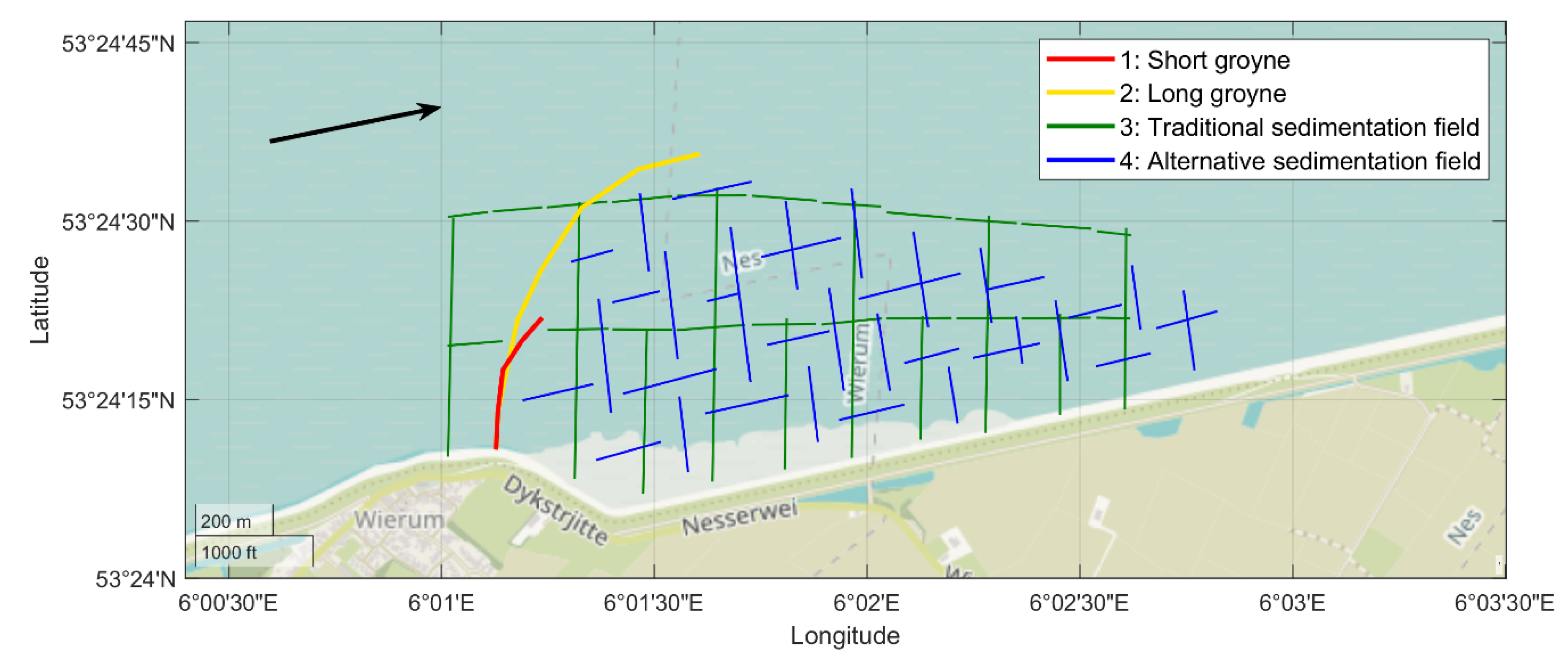
| Short | 1 | A short groyne of 2.5 m high representing a structure such as large groyne in Figure 3f. |
| Long | 2 | A long groyne of 2.5 m high, similar as Short above. |
| Long + Alternative | 2 + 4 | Combination of Long and an alternative sedimentation field, representing a conceptual design (Figure 3f). |
| Short + Traditional | 1 + 3 | Combination of Short and a traditional sedimentation field. This configuration of sedimentation fields is often used in the past (Figure 3c). |
| Mean Flow Velocity () | Mean Wave Height () | |||||
|---|---|---|---|---|---|---|
| Simulation | Storm | Calm | Total | Storm | Calm | Total |
| Default | 18.7 | 8.2 | 10.3 | 20.5 | 3.0 | 6.2 |
| Short | 17.5 | 7.9 | 9.9 | 19.9 | 2.8 | 5.9 |
| Long | 11.3 | 6.4 | 7.5 | 17.6 | 2.3 | 5.1 |
| Long + Alternative | 10.3 | 6.3 | 7.1 | 14.7 | 2.1 | 4.4 |
| Short + Traditional | 12.9 | 5.5 | 6.8 | 9.7 | 0.6 | 2.6 |
| Structure Name | Short | Long | Long + Alternative | Short + Traditional |
|---|---|---|---|---|
| Allowing accretion salt marsh | 1 | 2 | 3 | 4 |
| Reduced erosion marsh front | 4 | 3 | 2 | 1 |
| Accretion tidal flat | 3 | 2 | 4 | 1 |
| Stability tidal flat | 4 | 3 | 2 | 1 |
© 2020 by the authors. Licensee MDPI, Basel, Switzerland. This article is an open access article distributed under the terms and conditions of the Creative Commons Attribution (CC BY) license (http://creativecommons.org/licenses/by/4.0/).
Share and Cite
Siemes, R.W.A.; Borsje, B.W.; Daggenvoorde, R.J.; Hulscher, S.J.M.H. Artificial Structures Steer Morphological Development of Salt Marshes: A Model Study. J. Mar. Sci. Eng. 2020, 8, 326. https://doi.org/10.3390/jmse8050326
Siemes RWA, Borsje BW, Daggenvoorde RJ, Hulscher SJMH. Artificial Structures Steer Morphological Development of Salt Marshes: A Model Study. Journal of Marine Science and Engineering. 2020; 8(5):326. https://doi.org/10.3390/jmse8050326
Chicago/Turabian StyleSiemes, Rutger W. A., Bas W. Borsje, Roy J. Daggenvoorde, and Suzanne J. M. H. Hulscher. 2020. "Artificial Structures Steer Morphological Development of Salt Marshes: A Model Study" Journal of Marine Science and Engineering 8, no. 5: 326. https://doi.org/10.3390/jmse8050326
APA StyleSiemes, R. W. A., Borsje, B. W., Daggenvoorde, R. J., & Hulscher, S. J. M. H. (2020). Artificial Structures Steer Morphological Development of Salt Marshes: A Model Study. Journal of Marine Science and Engineering, 8(5), 326. https://doi.org/10.3390/jmse8050326