The Influence of the Chamber Configuration on the Hydrodynamic Efficiency of Oscillating Water Column Devices

Abstract

Based on the two-dimensional linear wave theory, the effects of the front wall thickness and the bottom profile of an Oscillating Water Column (OWC) device on its efficiency were analyzed. Using the potential flow approach, the solution of the associated boundary value problem was obtained via the boundary element method (BEM). Numerical results for several physical parameters and configurations were obtained. The effects of the front wall thickness on the efficiency are discussed in detail, then, various configurations of the chamber bottom are presented. A wider efficiency band was obtained with a thinner front wall. In a real scenario having a thinner front wall means that such a structure could have less capacity to withstand the impact of storm waves. Applying the model for the case of the Mutriku Wave Energy Plant (MWEP), findings showed that the proposed bottom profiles alter the efficiency curve slightly; higher periods of the incoming water waves were found. This could increase the efficiency of the device in the long-wave regime. Finally, the numerical results were compared with those available in the literature, and were found to be in good agreement.

1. Introduction

It has been suggested that wave power has the potential to provide most of the world’s electricity needs in the short term [1]. A wide variety of systems have been proposed, of which only a few have reached full-scale prototype deployments [2]. Among the deployed systems, the OWC system has been shown to be one of the most promising devices. It is probably the system that has been most studied and is one of the few to have been tested at full-scale. OWCs can be located offshore, near-shore or on the shoreline, and placed on the seabed or fixed to a rocky cliff [3]. Since the design and construction of OWCs are strongly site-dependent, their location and anchorage points are of the most critical aspects, as well as the most influential in economic terms.

In light of this, installing an OWC device into a breakwater was seen as a means to provide many benefits and thus encourage further development of OWC technology [4]. The breakwater provides shelter and contributes to coastal protection by reducing wave reflection. An OWC power plant within a breakwater has the advantage of being relatively easy to install and maintain, having no mooring systems and underwater electric cables. With construction and maintenance costs shared, and the operation of the power plant being easier, energy extraction is more cost-effective. Although the waves found near the coast are less energetic, this can, in part, be compensated by the natural concentration of wave energy due to shoaling, refraction and diffraction [5].

The first integrated breakwater-OWC system was built in the port of Sakata, Japan, in 1990 [6]. Subsequently, the Basque Energy Agency (Ente Vasco de la Energía or EVE for its acronym in Spanish) employed this concept in Mutriku, The Basque Country, Spain, opening the Mutriku Wave Energy Plant in July 2011, Figure 1. This plant consists of 16 units built onsite that are 4.5 m wide, 3.1 m depth, and 10 m high (above Maximum Equinoctial Spring Tide Low Water). For each unit, a hole of 0.75 m diameter leads to a Wells turbine and electrical generator of 18.5 kW [7], yielding the total 296 kW with a 100 m breakwater. The MWEP section of the breakwater is the first multiple OWC plant in the world and is currently the only OWC device in operation that regularly supplies power to the grid. However, regarding its performance, the initial expectations have not been met because of the poor design in some of the chambers that provide moderately different pressure at the inlet of their turbines [8]. This is because the breakwater that houses the Wells turbines was manly designed to maximizing the protection of Mutriku harbour and not for wave energy harnessing.

In this context, another factor contributing to the plant’s reduced electricity output could be the changes made to the front face of the original design. The area is regularly affected by severe storms and during the construction of the power plant, three storms hit the MWEP producing severe structural damage to a number of the OWC chambers [12]. As a consequence, the front face of the chambers was reinforced to withstand the wave loads, using prefabricated concrete slabs, so that now the thickness of the front wall has doubled the length of the chambers, Figure 2. This alteration was made to save the structure of the plant, but without considering the effect that this would have on the device performance. The main focus of this work is, therefore, the evaluation of the influence that the front wall thickness of an OWC-breakwater system has on its hydrodynamic performance as an OWC.

It is important to note that the success of the OWC system will depend on the coupling between the chamber and the power take-off (PTO) system. In this sense, a good turbine design, an effective control strategy and the matching of the turbine to the OWC collector to ensure efficient collector operation are essential [13]. Furthermore, the peak performance of most OWC systems occurs at resonance, which takes place when the incident wave frequency coincides with the natural frequency of the converter. Therefore, to operate optimally at resonance, the OWC chamber design plays a significant role to obtain higher efficiencies. Typically the chamber geometrical configuration is chosen to produce a column whose natural frequency of oscillation coincides with that of the most occurring wave at the location where the OWC will be installed [14]. In this sense, the variability of sea state conditions can influence the OWC feasibility, because, once installed, the size and shape of the structure can be hardly modified.

Over the last years, a variety of analytical, numerical and experimental techniques have been employed to study the effects of the geometrical configuration of an OWC on its hydrodynamic efficiency. Wang et al. [15] studied the hydrodynamic performance, both numerically and theoretically, of an OWC device with arbitrary topography near the shoreline. They reported that as the bottom slope increases, the peaks in capture-width ratios become lower frequency values, concluding that a change in water depth at the shoreline has a significant effect on the hydrodynamic performance of an OWC. The effect of front wall geometry on OWC hydrodynamic efficiency was analyzed by Thomas et al. [16]. Their experimental study concluded that the overall peak in hydrodynamic efficiency is not influenced greatly by the front wall geometry. Martins-rivas and Mei [17] presented a theoretical model for a cylindrical OWC installed on a cliff coast. It was found that air compressibility helps optimize the power absorption efficiency while the angle of incidence significantly affects the waves outside the chamber but not the averaged response inside or the capture length of energy absorption. Şentürk and Özdamar [18] carried out a theoretical analysis of an OWC which had a gap in its fully-submerged front wall. They showed that it is possible to increase the efficiency of an OWC with a surface piercing, barrier-type front wall when appropriate geometrical parameters are taken into consideration.

Rezanejad et al. [19] analyzed the impact of stepped bottom topography in the efficiency of a nearshore OWC device. They reported that there are significant effects when there is a stepped bottom profile outside of the chamber. Ning et al. [20] studied the performance of a fixed OWC device based on a time-domain higher-order BEM in a 2D fully nonlinear numerical wave flume. They investigated the hydrodynamic performance, with, and without, a bottom slope in the OWC chamber, and reported that the geometric parameters of the air chamber have a significant influence on hydrodynamic efficiency. The configuration of the bottom profile on the hydrodynamic performance of the OWC was investigated experimentally by Ashlin et al. [21]. Flat, circular, curved and sloped bottom profiles were tested in a wave flume. It was found that the OWC with a circular curved bottom profile was more effective in wave energy conversion, as was the wave amplification factor inside the chamber. The effects of the incident wave amplitude and geometric parameters on the hydrodynamic efficiency of a fixed OWC were investigated by Ning et al. [22]. They concluded that the incident wave amplitude and the bottom slope have a small influence on the resonant frequency, while the optimal hydrodynamic efficiency increases with an increase of bottom slope. A theoretical model based on linear potential flow theory to study the performance of a circular cylindrical OWC along a vertical coast/breakwater without the thin-wall restriction was proposed by [23]. The authors concluded that the incident wave direction and the thickness of the circular chamber wall both play an important role in the wave power captured by the OWC. By employing the eigenfunction matching method, Zheng et al. [24] developed a theoretical model to evaluate the hydrodynamic performance of multiple circular cylinder OWCs installed along a vertical straight coast. It was found that due to the effects of constructive wave interference from the OWCs array and the coast, the hydrodynamic performance of the OWC devices was enhanced significantly for a certain range of wave conditions. Zheng et al. [25] studied the effect of the radius of the entrance to the chamber and the finite wall thickness of the tubular-structure. They demonstrated that wave power extraction is greater with a thinner chamber wall thickness, mainly in terms of a broader primary band of efficiency curves. Using a coupled eigenfunction expansion—BEM—Koley and Trivedi [26] analyzed the hydrodynamic performance and efficiency of an OWC device placed on an undulated seabed. They concluded that the OWC structural design and bottom profile can significantly increase the hydrodynamic efficiency. A 2D BEM model for analyzing the OWC’s response in general bathymetry regions was carried out by [27]. They showed that the effects of the bottom slope and curvature on the OWC performance could be important, especially when the wave climate leads the site-specific optimal design to low resonance frequencies.

2. Aims and Methodology

In the specialized literature, there still remains a lot to be investigated regarding the improvement of the OWC efficiency by modifying its structural configuration. To the authors’ knowledge, a numerical study for analyzing the interaction of water waves with an OWC-breakwater system considering a wide front barrier has not been examined in the past. The fundamental hypothesis of the present work is that the hydrodynamic efficiency can be highly affected when a thick front barrier is employed. This reduction to the efficiency could be explained by the fact that the transfer of energy from the incoming wave to the internal free surface due to the orbital wave motion is reduced. A reduction in energy transmission then may lead to a decrease in the internal free surface oscillation for driving the air column, which consequently diminishes the output power.

Furthermore, by following the same idea of a wide front barrier but now considering the physical dimensions of a chamber in the MWEP, three different bottom profiles inside the chamber are then proposed to analyze their influence on the hydrodynamic efficiency. These proposed varying bottom profiles are a slope, a cycloid and an ellipse. This proposal is motivated by the fact that a curve bottom profile can exhibit better performance in terms of wave energy conversion and wave amplification inside the chamber, as it was experimentally studied by [21]. For this purpose, a numerical study for analyzing these curved profiles inside the chamber is also proposed.

Thus, this work examines the two-dimensional hydrodynamic interaction of ocean waves with an OWC device. Linear wave theory for a constant sea depth is employed and the viscous effects and the nonlinear air compressibility are neglected. The associated Boundary Value Problem (BVP) is then solved by the BEM employing three noded quadratic elements. The present formulation is novel in addressing the influence of a wide front wall and the use of BEM with a second-order discretization. The main interest of this work a) lies on the analysis of the bandwidth reduction on the efficiency curves due to an increment on the front wall thickness, and then, b) based on the geometric dimensions of the MWEP, to study alternatives for increasing the efficiency by considering a modification in the bottom profile inside the OWC chamber. Numerical estimates for the hydrodynamic efficiency and the radiation susceptance and radiation conductance coefficients are presented for a range of different parameters. Furthermore, numerical results for particular cases are validated with the previous results obtained by Evans and Porter [28] for a thin vertical surface-piercing barrier next to a vertical wall, and Şentürk and Özdamar [18] for an OWC with a gap on a fully submerged front wall.

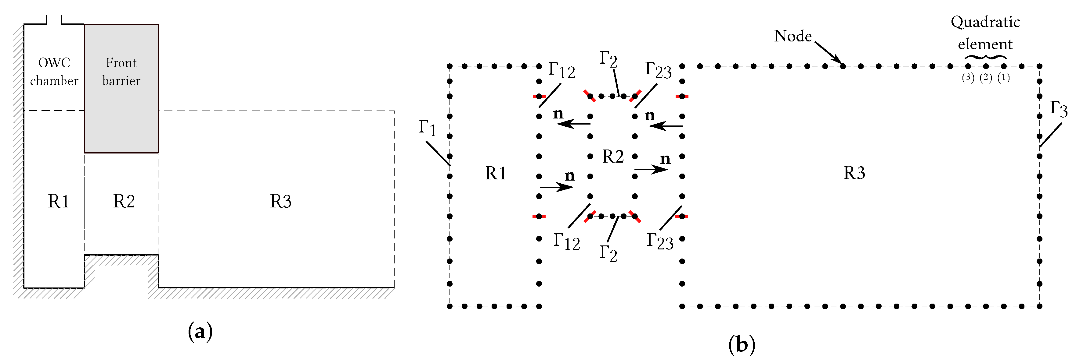
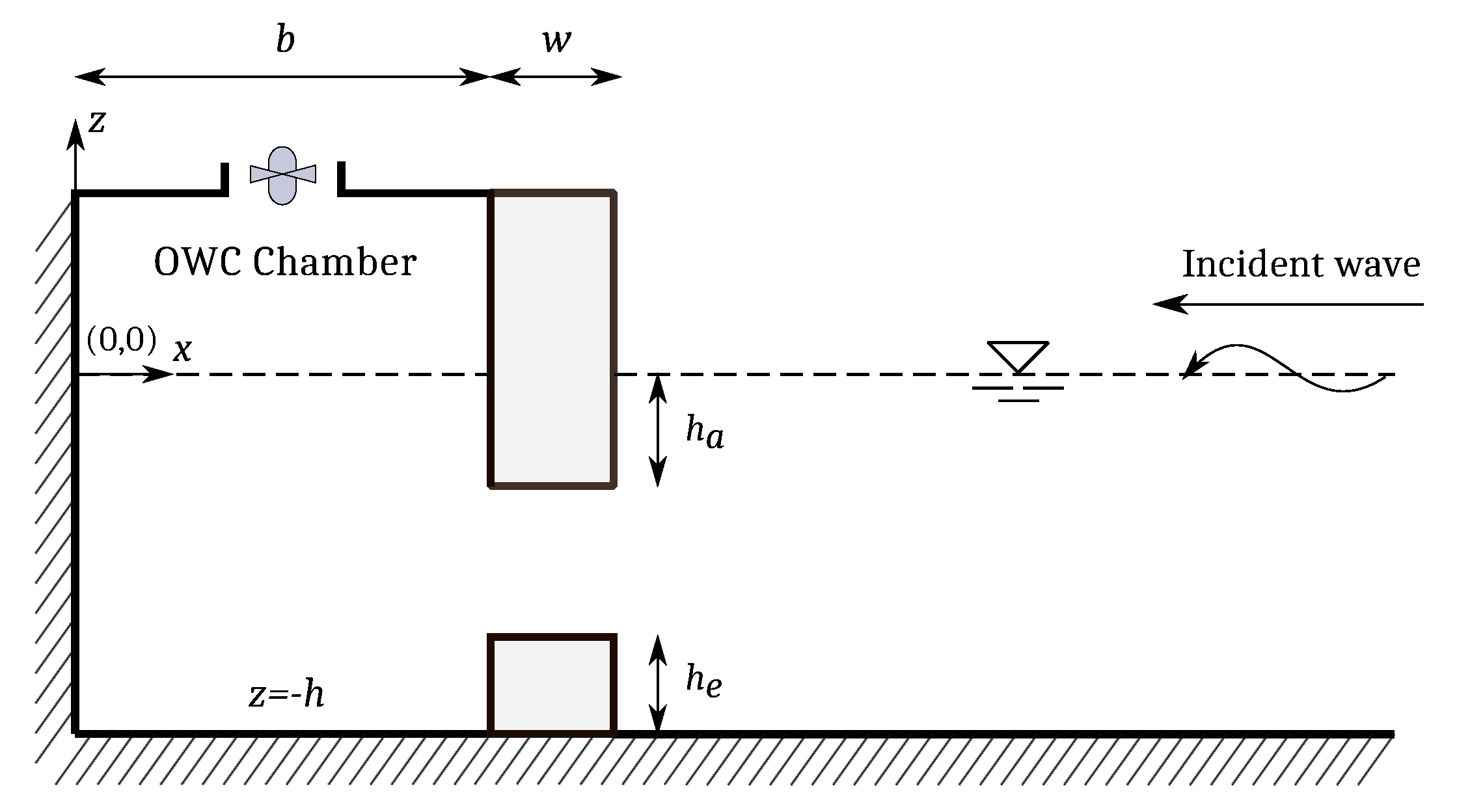
3. The Boundary-Value Problem

For the present study, the Cartesian coordinate system was chosen, with the $x-$axis corresponding to the opposite direction of the wave propagation and the $z-$axis corresponding to the upward direction. The origin of the coordinate system lies on the undisturbed free surface and the left-vertical wall inside the chamber. The OWC is this rigid wall, situated at $x=0$, extending down to the sea bottom and complemented by a vertical, surface-piercing barrier, at $x=b$, with a thickness w and a draft $h_a$, as shown in Figure 3. The front barrier is denoted by $L_b=\{(x,z):(x=b,-h_a\le z\le 0)\cup (b<x<b+w,z=-h_a)\cup (x=b+w,-h_a\le z\le 0)\}$, at the left side of the chamber entrance, the vertical length of the gap between the immersed tip of the barrier and the bottom is defined by $L_g=\{(x,z):x=b,-h_e\le z\le -h_a\}$, the rigid vertical wall by $S_w=\{(x,z):x=0,-h<z<0\}$, the internal free surface inside the water column by $S_i=\{(x,z):0\le x\le b,z=0\}$, the external free surface by $S_f=\{(x,z):b+w\le x\le \infty ,z=0\}$ and the bottom by $S_b=\{(x,z):(0<x<b,z=-h)\cup (x=b,-h<z<-h_e)\cup (b<x<b+w,z=-h_e)\cup (x=b+w,-h<z<-h_e)\cup (b+w<x<\infty ,z=-h)\}$.

The fluid is assumed to be inviscid and incompressible and linear wave theory is applied, ignoring the effect of surface tension. By assuming an irrotational flow and simple harmonic in time with angular frequency $\omega$, there is thus a velocity potential $\mathsf{\Phi }(x,z,t)$ with $\mathsf{\Phi }(x,z,t)=\mathrm{Re}\left\{\varphi (x,z){\mathrm{e}}^{-\mathrm{i}\omega t}\right\}$, where Re$\left\{\right\}$ denotes the real part of a complex expression and t is the time. The spatial velocity potential $\varphi$ then satisfies the Laplace equation

$$\frac{{\partial }^2\varphi }{\partial x^2}+\frac{{\partial }^2\varphi }{\partial z^2}=0,$$

(1)

along with the no-flow boundary condition on the solid boundaries such as the barrier, the rigid vertical wall and the bottom described by

$$\frac{\partial \varphi }{\partial n}=0\mathrm{for}(x,z)\in S_b,S_w\mathrm{and}{L}_b,$$

(2)

together with the continuity of pressure and horizontal velocity given by

$${\varphi }_{-}={\varphi }_{+}\mathrm{and}{\frac{\partial \varphi }{\partial x}}_{-}=\begin{array}{c}\hfill -\end{array}{\frac{\partial \varphi }{\partial x}}_{+}\mathrm{for}(x,z)\in L_g\mathrm{on}\left\{\begin{array}{c}x=b,\hfill \\ x=b+w.\hfill \end{array}\right.$$

(3)

Inside the chamber, by imposing a pressure distribution over the internal free surface $P\left(t\right)$ and after considering simple harmonic motions for the free surface $\overline{\eta }=\mathrm{Re}\left\{\zeta {\mathrm{e}}^{-\mathrm{i}\omega t}\right\}$ and $P\left(t\right)=\mathrm{Re}\left\{p{\mathrm{e}}^{-\mathrm{i}\omega t}\right\}$, the dynamic and kinematic free surface boundary conditions are

$$\varphi +\frac{\mathrm{i}g}{\omega }\zeta =-\frac{\mathrm{i}}{\rho \omega }p\mathrm{on}z=0,0<x<b,$$

(4a)

$$\frac{\partial \varphi }{\partial z}+\mathrm{i}\omega \zeta =0\mathrm{on}z=0,0<x<b,$$

(4b)

and on the external free surface with $p=0$

$$\varphi +\frac{\mathrm{i}g}{\omega }\zeta =0\mathrm{on}z=0,b<x<\infty ,$$

(5a)

$$\frac{\partial \varphi }{\partial z}+\mathrm{i}\omega \zeta =0\mathrm{on}z=0,b<x<\infty .$$

(5b)

Thus, by combining Equations (4) and (5), the internal and external linearized free surface boundary conditions are

$$\frac{\partial \varphi }{\partial z}-K\varphi =\left\{\begin{array}{cc}\frac{\mathrm{i}\omega p}{\rho g}\hfill & \mathrm{on}z=0,0<x<b,\hfill \\ 0\hfill & \mathrm{on}z=0,b<x<\infty ,\hfill \end{array}\right.$$

(6)

respectively, where $K={\omega }^2/g$, with g being the gravitational constant and $\rho$ the seawater density.

Here, as described by [28], the potential is decomposed into two parts as follows

$$\varphi (x,z)={\varphi }^S+\frac{\mathrm{i}\omega p}{\rho g}{\varphi }^R.$$

(7)

The scattered potential ${\varphi }^S$ represents the solution of the scattering of an incident wave coming from $x=+\infty$ in the absence of an imposed pressure on the internal free surface inside the chamber, satisfying Equations (1)–(6) with $p=0$; while the radiated potential ${\varphi }^R$ represents the solution of the radiation problem due to the pressure imposed on the internal free surface and satisfies Equations (1)–(6) with Equation (6) replaced by

$$\frac{\partial {\varphi }^R}{\partial z}-K{\varphi }^R=1\mathrm{on}z=0,0<x<b,$$

(8)

which is due to an oscillating pressure distribution on the internal free surface in the absence of incoming waves.

The Sommerfeld radiation condition describes the far field boundary condition for the diffraction and radiation problems as follows:

$$\frac{\partial {\varphi }^{D,R}}{\partial x}-\mathrm{i}k{\varphi }^{D,R}=0\mathrm{as}x\to +\infty ,$$

(9)

where ${\varphi }^D$ represents the diffracted potential that together with the incident potential ${\varphi }^I$ composed the scattered potential ${\varphi }^S$, while k represents the wave number and is the real root of the wave dispersion relation given by

$${\omega }^2=gktanhkh,$$

(10)

whose solution of this expression can be easily determined by a root-finding algorithm.

On the other hand, the time harmonic induced volume flux across the internal free surface, $Q\left(t\right)=\mathrm{Re}\left\{q{e}^{-\mathrm{i}\omega t}\right\}$ (see [28]) is given by

$$q={\int }_{S_i}\frac{\partial \varphi }{\partial z}dx=q^S+\frac{\mathrm{i}\omega p}{\rho g}{q}^R,$$

(11)

where $q^S$ and $q^R$ are the volume fluxes across $S_i$ in the scattering and radiation problems, respectively. Thus, by using the continuity of volume flux across the internal free surface and the gap between the barrier tip and the sea bottom, we obtain

$$q^{S,R}={\int }_{S_i}\frac{\partial {\varphi }^{S,R}}{\partial z}dx=\begin{array}{c}\hfill -\end{array}{\int }_{L_g}\frac{\partial {\varphi }^{S,R}}{\partial x}dz.$$

(12)

Finally, the volume flux $q^R$ for the radiation problem is separated into real and imaginary parts as follows

$$\frac{i\omega p}{\rho g}{q}^R=-\left(\tilde{B}-\mathrm{i}\tilde{A}\right)p=-Zp,$$

(13)

where $Z=\tilde{B}-\mathrm{i}\tilde{A}$ is a complex admittance and $\tilde{A}$ and $\tilde{B}$ are analogous to the added mass and the radiation damping coefficients of the forced oscillation of a rigid body system immersed in an ideal fluid and, following [28], are called the radiation susceptance and the radiation conductance parameters, respectively, described by

$$\tilde{A}=\frac{\omega }{\rho g}\mathrm{Re}\left\{q^R\right\},$$

(14a)

$$\tilde{B}=\frac{\omega }{\rho g}\mathrm{Im}\left\{q^R\right\},$$

(14b)

where Im$\left\{\right\}$ denotes the imaginary part of a complex expression.

Efficiency Relations

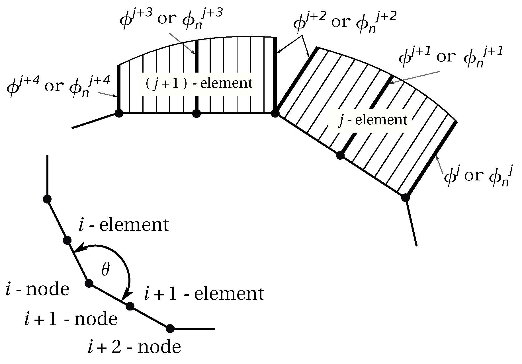
Since in practice it may be easier to control the volume flux through the turbines than the pressure drop across it [29], a linear relationship between these two without a phase lag is assumed,

$$q=\left(\mathsf{\Lambda }-\mathrm{i}\varrho \right)p,$$

(15)

where $\mathsf{\Lambda }$ is a real control parameter, related to the damping induced to the airflow by the linear turbine and $\varrho =\omega V_0/\left(\gamma p_a\right)$ represents the effect of compressibility of air in the chamber with $V_0$ being the air volume inside the chamber, $\gamma$ the specific heat ratio of air equal to 1.4 and $p_a$ the atmospheric air pressure [30]. The sign in $\mathsf{\Lambda }$ is taken to be positive since, in contrast to Equation (13), the pressure forces and volume fluxes are both measured vertically upwards. Equation (15) assumes that the pressure inside the chamber is uniform and the air exits to the atmosphere through the turbine, a characteristic of Wells turbines that has been widely investigated for OWC devices. Using Equations (11), (13) and (15) an expression for the pressure in the chamber can be found

$$p=\frac{q^S}{\mathsf{\Lambda }+Z-\mathrm{i}\varrho }.$$

(16)

The total rate of working of the pressure forces inside the OWC is basically $Q\left(t\right)\times P\left(t\right)$. By averaging this over one period, the mean power absorbed per unit width of pressure distribution is obtained

$$W=\frac{1}{2}\mathrm{Re}\left\{p^{*}q\right\},$$

(17)

where ${}^{*}$ denotes complex conjugate. Now, by using Equations (11) and (13) on this last expression, we obtain

$$W=\frac{1}{2}\mathrm{Re}\left\{p^{*}\left(q^S-Zp\right)\right\}=\frac{1}{2}\left(\mathrm{Re}\left\{p^{*}{q}^S\right\}-\tilde{B}{\left|p\right|}^2\right).$$

(18)

The expression (18) can be re-written in the form

$$W=\frac{1}{8}{q}^{S*}{q}^S{\tilde{B}}^{-1}-\frac{1}{2}\tilde{B}{\left(p-\frac{q^S}{2\tilde{B}}\right)}^{*}\left(p-\frac{q^S}{2\tilde{B}}\right)=\frac{|q^S{|}^2}{8\tilde{B}}-\frac{\tilde{B}}{2}{\left|p-\frac{q^S}{2\tilde{B}}\right|}^2,$$

(19)

where if ${\tilde{B}}^{-1}$ exists, the maximum work is

$$W_{max}=\frac{|q^S{|}^2}{8\tilde{B}},$$

(20)

when

$$p=\frac{q^S}{2\tilde{B}},$$

(21)

showing that $\mathsf{\Lambda }={\left(Z-\mathrm{i}\varrho \right)}^{*}$ for maximum power.

By combining previous Equations (16) and (19), it is finally obtained Equation (22):

$$W=\frac{|q^S{|}^2}{8\tilde{B}}\left[1-{\left(\frac{|\mathsf{\Lambda }-Z+\mathrm{i}\varrho |}{|\mathsf{\Lambda }+Z-\mathrm{i}\varrho |}\right)}^2\right].$$

(22)

Now, in order to optimize the power conversion efficiency, the last term in the square brackets must be minimized. As in Şentürk and Özdamar [18], this can be done by finding the optimum value of $\mathsf{\Lambda }$, which can be evaluated by applying zero value to the derivative for the squared-right term inside the brackets of Equation (22) with respect to $\mathsf{\Lambda }$, and thus obtaining

$${\mathsf{\Lambda }}_{opt}=|Z-\mathrm{i}\varrho |={\left({\tilde{B}}^2+{\left(\tilde{A}+\varrho \right)}^2\right)}^{1/2}.$$

(23)

Therefore, the maximum value of extracted work at this condition becomes,

$$W_{opt}=\frac{|q^S{|}^2}{8\tilde{B}}\left[1-\frac{{\mathsf{\Lambda }}_{opt}-\tilde{B}}{{\mathsf{\Lambda }}_{opt}+\tilde{B}}\right],$$

(24)

where $\tilde{A}$, $\tilde{B}$ and $\mathsf{\Lambda }$ are function of the angular frequency $\omega$ which means that for each wave frequency, the turbine parameter must be altered appropriately to satisfy Equation (23).

Thus, the expression for maximum efficiency is expressed as

$${\eta }_{max}=\frac{W_{opt}}{W_{max}}=\frac{2\tilde{B}}{{\mathsf{\Lambda }}_{opt}+\tilde{B}},$$

(25)

where the maximum hydrodynamic efficiency is bounded by $0\le {\eta }_{max}\le 1$. From expression (23), it is clear that when the radiation susceptance parameter is zero and the air compressibility term is neglected, it results in ${\mathsf{\Lambda }}_{opt}=\tilde{B}$, $W_{opt}=W_{max}$ and ${\eta }_{max}=1$, thus implying that the device has effectively absorbed all of the incident wave energy. In this situation, the free surface inside the OWC chamber is characterized by a piston-like resonant mode and the PTO damping optimization is satisfied [31]. To remain at this condition, the rate of energy extraction must equate to the rate of radiation damping while the internal free surface must remain in a state of resonance. Physically, this requires that the radiated waves, resulting from the oscillatory heave motion of the internal free surface, superpose and cancel the incident and scattered waves; in this instance, the device has thereby captured all of the incident wave energy [16].

Now, as in [28] the non-dimensionalised quantities $\mu$ and $\nu$ to represent the radiation susceptance and radiation conductance coefficients are defined as

$$\mu =\frac{\rho g}{\omega b}\tilde{A},$$

(26a)

$$\nu =\frac{\rho g}{\omega b}\tilde{B},$$

(26b)

respectively, where the radiation conductance coefficient $\nu$ is related to the transfer of energy into the system, while the radiation susceptance coefficient $\mu$ to the energy that remains un-captured [19].

Therefore, by substituting these coefficients into Equation (25), the efficiency ${\eta }_{max}$ is

$${\eta }_{max}=\frac{2}{{\left(1+{\left(\frac{\mu }{\nu }\right)}^2\right)}^{1/2}+1},$$

(27)

which is independent of the incident wave power and only depends on the radiation solution of the volume flux q.

4. Solution

In this section, the BEM is used to solve the BVP in the frequency domain. In order to solve the governing equation together with the appropriated boundary conditions, a quadratic distribution of variables along each element is considered. The integral representation of the solution for the Laplace equation Equation (1) at any point source $\overline{P}$ inside the domain $\mathsf{\Omega }$ in terms of the boundary values of $\varphi$ and $\partial \varphi /\partial n$ is given by

$$\alpha \left(\overline{P}\right)\varphi \left(\overline{P}\right)+{\int }_{\mathsf{\Gamma }}\varphi \left(\overline{q}\right)\frac{\partial \psi (\overline{P},\overline{q})}{\partial n_{\overline{q}}}d{\mathsf{\Gamma }}_{\overline{q}}={\int }_{\mathsf{\Gamma }}\psi (\overline{P},\overline{q})\frac{\partial \varphi \left(\overline{q}\right)}{\partial n_{\overline{q}}}d{\mathsf{\Gamma }}_{\overline{q}},$$

(28)

where $\varphi$ is the unknown flow potential; $\partial \varphi /\partial n$ is the derivative of the potential relative to normal unit vector on the boundary $\mathsf{\Gamma }$; $d\mathsf{\Gamma }$ is the length of an infinitesimal piece of $\mathsf{\Gamma }$; $\overline{q}$ an arbitrary point; while $\psi$ and $\partial \psi /\partial n$ are the fundamental solution of Laplace equation and its normal derivative at point $\overline{q}$ of the boundary, respectively; and $\alpha =\theta /2\pi$, where $\theta$ is the internal angle of the corner in radians [32].

The fundamental solution of Laplace equation is given by

$$\psi =\frac{1}{2\pi }lnr,$$

(29)

where r is the distance between the source $\overline{P}$ and the arbitrary point $\overline{q}$.

Now, discretizing the boundary into a series of $NE$ elements, Equation (28) can be written as

$${\alpha }^i{\varphi }^i+\sum _{j=1}^{NE}{\int }_{\mathsf{\Gamma }}\varphi \frac{\partial \psi }{\partial n}d\mathsf{\Gamma }=\sum _{j=1}^{NE}{\int }_{\mathsf{\Gamma }}\psi \frac{\partial \varphi }{\partial n}d\mathsf{\Gamma }.$$

(30)

In order to define the values of $\varphi$ and $\partial \varphi /\partial n$ on each element, three noded quadratic elements are employed, Figure 4. The variables $\varphi$ and $\partial \varphi /\partial n$ are thus written in terms of interpolation functions, ${\widehat{\phi }}_{1,2,3}$, which are function of a homogeneous coordinate $\xi$ as follows

$$\varphi \left(\xi \right)={\widehat{\phi }}_1{\varphi }^1+{\widehat{\phi }}_2{\varphi }^2+{\widehat{\phi }}_3{\varphi }^3,$$

(31a)

$$\frac{\partial \varphi \left(\xi \right)}{\partial n}={\widehat{\phi }}_1\frac{\partial {\varphi }^1}{\partial n}+{\widehat{\phi }}_2\frac{\partial {\varphi }^2}{\partial n}+{\widehat{\phi }}_3\frac{\partial {\varphi }^3}{\partial n},$$

(31b)

where the superscript indicates the number of the node, while the interpolation functions are given by

$${\widehat{\phi }}_1=\frac{1}{2}\xi \left(\xi -1\right),$$

(32a)

$${\widehat{\phi }}_2=\frac{1}{2}\left(1-\xi \right)\left(1+\xi \right),$$

(32b)

$${\widehat{\phi }}_3=\frac{1}{2}\xi \left(1+\xi \right),$$

(32c)

with the dimensionless coordinate $\xi$ varying from −1 to 1. Now, carrying out the integrals from Equation (30) over an element j, these can be written as

$${\int }_{{\mathsf{\Gamma }}_j}\varphi \frac{\partial \psi }{\partial n}d\mathsf{\Gamma }=\left[{\int }_{{\mathsf{\Gamma }}_j}{\widehat{\phi }}_1\frac{\partial \psi }{\partial n}d\mathsf{\Gamma },{\int }_{{\mathsf{\Gamma }}_j}{\widehat{\phi }}_2\frac{\partial \psi }{\partial n}d\mathsf{\Gamma },{\int }_{{\mathsf{\Gamma }}_j}{\widehat{\phi }}_3\frac{\partial \psi }{\partial n}d\mathsf{\Gamma }\right]·\left\{\begin{array}{c}{\varphi }^1\\ {\varphi }^2\\ {\varphi }^3\end{array}\right\},$$

(33)

and

$${\int }_{{\mathsf{\Gamma }}_j}\psi \frac{\partial \varphi }{\partial n}d\mathsf{\Gamma }=\left[{\int }_{{\mathsf{\Gamma }}_j}{\widehat{\phi }}_1\psi d\mathsf{\Gamma },{\int }_{{\mathsf{\Gamma }}_j}{\widehat{\phi }}_2\psi d\mathsf{\Gamma },{\int }_{{\mathsf{\Gamma }}_j}{\widehat{\phi }}_3\psi d\mathsf{\Gamma }\right]·\left\{\begin{array}{c}\frac{\partial {\varphi }^1}{\partial n}\\ \frac{\partial {\varphi }^2}{\partial n}\\ \frac{\partial {\varphi }^3}{\partial n}\end{array}\right\}.$$

(34)

Here, it is observed that in order to solve the integrals Equations (33) and (34), the calculation of the Jacobian is required since they are a function of the boundary $\mathsf{\Gamma }$ in the $x-z$ plane, while the interpolation functions are a function of $\xi$. This transformation is given by

$$d\mathsf{\Gamma }=\left[\sqrt{{\left(\frac{dx}{d\xi }\right)}^2+{\left(\frac{dz}{d\xi }\right)}^2}\right]d\xi =\left|J\right|d\xi ,$$

(35)

where J indicates the Jacobian and can then be substituted into Equations (33) and (34). Additionally, in order to calculate the value of Equation (35), the variation of the x and z coordinates in terms of $\xi$ must be also known. This can be carried out in the same way as the variables $\varphi$ and $\partial \varphi /\partial n$, with the use of the quadratic interpolation defined by

$$x={\widehat{\phi }}_1{x}^1+{\widehat{\phi }}_2{x}^2+{\widehat{\phi }}_3{x}^3,$$

(36a)

$$z={\widehat{\phi }}_1{z}^1+{\widehat{\phi }}_2{z}^2+{\widehat{\phi }}_3{z}^3,$$

(36b)

where again the superscript indicates the number of the node. Thus, Equation (30) can be written as

$${\alpha }^i{\varphi }^i+\sum _{j=1}^{NE}\left[h_1^{ij},h_2^{ij},h_3^{ij}\right]·{\left\{\begin{array}{c}{\varphi }^1\\ {\varphi }^2\\ {\varphi }^3\end{array}\right\}}^j=\sum _{j=1}^{NE}\left[g_1^{ij},g_2^{ij},g_3^{ij}\right]·{\left\{\begin{array}{c}{\varphi }_n^1\\ {\varphi }_n^2\\ {\varphi }_n^3\end{array}\right\}}^j,$$

(37)

where

$$h_k^{ij}={\int }_{-1}^1{\widehat{\phi }}_k\left(\xi \right)\frac{\partial \psi }{\partial n}\left|J\right|d\xi ,$$

(38a)

$$g_k^{ij}={\int }_{-1}^1{\widehat{\phi }}_k\left(\xi \right)\psi \left|J\right|d\xi ,$$

(38b)

with $k=1,$ 2 and 3 and $h_k^{ij}$ and $g_k^{ij}$ are estimated by using a Gauss integration method with ten points to account for the quadratic variation of the element geometry, the potential and flux. More details regarding the numerical procedure for solving these integrals can be found in [33,34].

Furthermore, as explained by [33], in order to consider the possibility of having different values of ${\varphi }_n$ at node 3 of an element and at node 1 of the next adjoining element, the fluxes are arranged in a 3$\times NE$ array where a position is held for each nodal value of every element. However, in the case of the potential $\varphi$, its value is always considered unique in the connection between two elements. Therefore, the values of $\varphi$ can be arranged in an N array, where N is the number of nodes equal to $2NE$ for closed boundaries. Thus, Equations (37) can be written as

$${\alpha }^i{\varphi }^i+\left[{\widehat{H}}^{i1},\dots {\widehat{H}}^{iN}\right]·{\left\{\begin{array}{c}{\varphi }^1\\ ⋮\\ {\varphi }^N\end{array}\right\}}^j=\left[G^{i1},\dots G^{iNE}\right]·{\left\{\begin{array}{c}{\left[\begin{array}{c}{\varphi }_n^1\\ {\varphi }_n^2\\ {\varphi }_n^3\end{array}\right]}^1\\ ⋮\\ {\left[\begin{array}{c}{\varphi }_n^1\\ {\varphi }_n^2\\ {\varphi }_n^3\end{array}\right]}^{NE}\end{array}\right\}}^j,$$

(39)

with ${\widehat{H}}^{ij}$ being equal to the $h_1$ term of an element plus the $h_3$ term of the previous element for odd nodes and equal to the $h_2$ term of the corresponding element for the central nodes. On the other hand, $G^{ij}$ are 1 × 3 matrices with the elements $\left[g_1^{ij},g_2^{ij},g_3^{ij}\right]$. Therefore, the whole system of equations can be simply written as follows

$$\mathbf{H}\mathsf{\Phi }=\mathbf{G}{\mathsf{\Phi }}_{\mathbf{n}},$$

(40)

where $\mathbf{H}$ is a square matrix $N\times N$, $\mathsf{\Phi }$ is an $N\times 1$ vector, $\mathbf{G}$ is a rectangular matrix $N\times 3NE$ and ${\mathsf{\Phi }}_{\mathbf{n}}$ is an $3NE\times 1$ vector.

Furthermore, as previously described by [19], in order to avoid the numerical errors arising from the cases where a very thin front wall of the device is considered, the method of subdomains is used to solve the BVP by applying the BEM separately to each of its regions [32,35]. The domain is then divided into three separate regions which have a common interface boundary on both lateral sides of the front wall as shown in Figure 5a. For each subdomain the following vectors are defined: in region R1

• ${\mathsf{\Phi }}_1^1$, ${{\mathsf{\Phi }}_{\mathbf{n}}}_1^1$ Nodal values on ${\mathsf{\Gamma }}_1$ of the external boundary.
• ${\mathsf{\Phi }}_{12}^1$, ${{\mathsf{\Phi }}_{\mathbf{n}}}_{12}^1$ Nodal values on the interface ${\mathsf{\Gamma }}_{12}$,

where the superscript denotes the region, while the subscript denotes the corresponding external boundary or interface. The number of the nodal points on ${\mathsf{\Gamma }}_1$ and ${\mathsf{\Gamma }}_{12}$ are $N_1$ and $N_{12}$, respectively. In region R2

• ${\mathsf{\Phi }}_2^2$, ${{\mathsf{\Phi }}_{\mathbf{n}}}_2^2$ Nodal values on ${\mathsf{\Gamma }}_2$ of the external boundary.
• ${\mathsf{\Phi }}_{12}^2$, ${{\mathsf{\Phi }}_{\mathbf{n}}}_{12}^2$ Nodal values on the interface ${\mathsf{\Gamma }}_{12}$.
• ${\mathsf{\Phi }}_{23}^2$, ${{\mathsf{\Phi }}_{\mathbf{n}}}_{23}^2$ Nodal values on the interface ${\mathsf{\Gamma }}_{23}$,

where the number of the nodal points on ${\mathsf{\Gamma }}_2$, ${\mathsf{\Gamma }}_{12}$ and ${\mathsf{\Gamma }}_{23}$ are $N_2$, $N_{12}$ and $N_{23}$, respectively. In region R3

• ${\mathsf{\Phi }}_3^3$, ${{\mathsf{\Phi }}_{\mathbf{n}}}_3^2$ Nodal values on ${\mathsf{\Gamma }}_3$ of the external boundary.
• ${\mathsf{\Phi }}_{23}^2$, ${{\mathsf{\Phi }}_{\mathbf{n}}}_{23}^2$ Nodal values on the interface ${\mathsf{\Gamma }}_{23}$,

with $N_3$ and $N_{23}$ being the number of the nodal points on ${\mathsf{\Gamma }}_3$ and ${\mathsf{\Gamma }}_{23}$, respectively.

Since $\varphi$ is unknown on either side of the interfaces ${\mathsf{\Gamma }}_{12}$ and ${\mathsf{\Gamma }}_{23}$, the number of boundary unknowns in each subdomain is:

• Region 1: $N_1$ on ${\mathsf{\Gamma }}_1$ and $N_{12}$ on ${\mathsf{\Gamma }}_{12}$.
• Region 2: $N_2$ on ${\mathsf{\Gamma }}_2$, $N_{12}$ on ${\mathsf{\Gamma }}_{12}$ and $N_{23}$ on ${\mathsf{\Gamma }}_{23}$.
• Region 3: $N_3$ on ${\mathsf{\Gamma }}_3$ and $N_{23}$ on ${\mathsf{\Gamma }}_{23}$.

On the other hand, for ${\varphi }_n$, which is defined on the three nodes of each element, it is given by:

• Region 1: $M_1=3N{E}_1$ on ${\mathsf{\Gamma }}_1$ and $M_{12}=3N{E}_{12}$ on ${\mathsf{\Gamma }}_{12}$.
• Region 2: $M_2=3N{E}_2$ on ${\mathsf{\Gamma }}_2$, $M_{12}=3N{E}_{12}$ on ${\mathsf{\Gamma }}_{12}$ and $M_{23}=3N{E}_{23}$ on ${\mathsf{\Gamma }}_{23}$.
• Region 3: $M_3=3N{E}_3$ on ${\mathsf{\Gamma }}_3$ and $M_{23}=3N{E}_{23}$ on ${\mathsf{\Gamma }}_{23}$,

where $N{E}_j$ denotes the number of elements depending on the boundary or interface.

Furthermore, in order to match the regions and to obtain the same number of unknowns and equations, the physical consideration of continuity of the potential and flux at the interfaces Equation (3) should be made. Thus, assuming that the nodes in ${\mathsf{\Gamma }}_{12}$ of $R1$ and $R2$, and the nodes in ${\mathsf{\Gamma }}_{23}$ of $R2$ and $R3$ are in perfect contact, Figure 5b, the following physical consideration at the interfaces can be made:

• Continuity of the potential: The values of the potential on each side of the interface separating two subdomains must be equal

  $$\left\{\begin{array}{cc}{\mathsf{\Phi }}_{12}^1\hfill & ={\mathsf{\Phi }}_{12}^2,\hfill \\ {\mathsf{\Phi }}_{23}^2\hfill & ={\mathsf{\Phi }}_{23}^3.\hfill \end{array}\right.$$

  (41)
• Continuity of the flux: The outcoming flux from one subdomain is equal to the incoming flux in the adjacent subdomain. Thus, the flux along the normal of the interface requires

  $$\left\{\begin{array}{cc}{{\mathsf{\Phi }}_{\mathbf{n}}}_{12}^1\hfill & =-{{\mathsf{\Phi }}_{\mathbf{n}}}_{12}^2,\hfill \\ {{\mathsf{\Phi }}_{\mathbf{n}}}_{23}^2\hfill & =-{{\mathsf{\Phi }}_{\mathbf{n}}}_{23}^3,\hfill \end{array}\right.$$

  (42)

  where the minus signs in the right hand side of Equation (42) indicate that the two flux vectors at the common interface of adjacent subdomains are in opposite directions.

Therefore, the matrix equation for each boundary subdomain is as follows: for the boundary subdomain $R1$

$$\left[\begin{array}{cc}{\left[H\right]}_1^1& {\left[H\right]}_{12}^1\end{array}\right]\left[\begin{array}{c}{\mathsf{\Phi }}_1^1\\ {\mathsf{\Phi }}_{12}^1\end{array}\right]=\left[\begin{array}{cc}{\left[G\right]}_1^1& {\left[G\right]}_{12}^1\end{array}\right]\left[\begin{array}{c}{{\mathsf{\Phi }}_{\mathbf{n}}}_1^1\\ {{\mathsf{\Phi }}_{\mathbf{n}}}_{12}^1\end{array}\right],$$

(43)

while for the boundary subdomain $R2$

$$\left[\begin{array}{ccc}{\left[H\right]}_{12}^2& {\left[H\right]}_2^2& {\left[H\right]}_{23}^2\end{array}\right]\left[\begin{array}{c}{\mathsf{\Phi }}_{12}^2\\ {\mathsf{\Phi }}_2^2\\ {\mathsf{\Phi }}_{23}^2\end{array}\right]=\left[\begin{array}{ccc}{\left[G\right]}_{12}^2& {\left[G\right]}_2^2& {\left[G\right]}_{23}^2\end{array}\right]\left[\begin{array}{c}{{\mathsf{\Phi }}_{\mathbf{n}}}_{12}^2\\ {{\mathsf{\Phi }}_{\mathbf{n}}}_2^2\\ {{\mathsf{\Phi }}_{\mathbf{n}}}_{23}^2\end{array}\right],$$

(44)

and for the boundary subdomain $R3$

$$\left[\begin{array}{cc}{\left[H\right]}_3^3& {\left[H\right]}_{23}^3\end{array}\right]\left[\begin{array}{c}{\mathsf{\Phi }}_3^3\\ {\mathsf{\Phi }}_{23}^3\end{array}\right]=\left[\begin{array}{cc}{\left[G\right]}_3^3& {\left[G\right]}_{23}^3\end{array}\right]\left[\begin{array}{c}{{\mathsf{\Phi }}_{\mathbf{n}}}_3^3\\ {{\mathsf{\Phi }}_{\mathbf{n}}}_{23}^3\end{array}\right].$$

(45)

Equations (43)–(45) of the three subdomains may then be combined in a single matrix equation as

$$\begin{array}{c}\left[\begin{array}{ccccccc}{\left[H\right]}_1^1& {\left[H\right]}_{12}^1& 0& 0& 0& 0& 0\\ 0& 0& {\left[H\right]}_2^2& {\left[H\right]}_{12}^2& {\left[H\right]}_{23}^2& 0& 0\\ 0& 0& 0& 0& 0& {\left[H\right]}_3^3& {\left[H\right]}_{23}^3\end{array}\right]\left[\begin{array}{c}{\mathsf{\Phi }}_1^1\\ {\mathsf{\Phi }}_{12}^1\\ {\mathsf{\Phi }}_2^2\\ {\mathsf{\Phi }}_{12}^2\\ {\mathsf{\Phi }}_{23}^2\\ {\mathsf{\Phi }}_3^3\\ {\mathsf{\Phi }}_{23}^3\end{array}\right]=\hfill \\ \hfill \left[\begin{array}{ccccccc}{\left[G\right]}_1^1& {\left[G\right]}_{12}^1& 0& 0& 0& 0& 0\\ 0& 0& {\left[G\right]}_2^2& {\left[G\right]}_{12}^2& {\left[G\right]}_{23}^2& 0& 0\\ 0& 0& 0& 0& 0& {\left[G\right]}_3^3& {\left[G\right]}_{23}^3\end{array}\right]\left[\begin{array}{c}{{\mathsf{\Phi }}_{\mathbf{n}}}_1^1\\ {{\mathsf{\Phi }}_{\mathbf{n}}}_{12}^1\\ {{\mathsf{\Phi }}_{\mathbf{n}}}_2^2\\ {{\mathsf{\Phi }}_{\mathbf{n}}}_{12}^2\\ {{\mathsf{\Phi }}_{\mathbf{n}}}_{23}^2\\ {{\mathsf{\Phi }}_{\mathbf{n}}}_3^3\\ {{\mathsf{\Phi }}_{\mathbf{n}}}_{23}^3\end{array}\right],\end{array}$$

(46)

where the left-hand side matrix and vector have dimensions of $N\times N$ and $N\times 1$, respectively, with $N=N_1+N_2+N_3+2N_{12}+2N_{23}$, while the right-hand side matrix and vector of $N\times 3NE$ and $3NE\times 1$, respectively, with $3NE=M_1+M_2+M_3+2M_{12}+2M_{23}$. Now, since the nodes on ${\mathsf{\Gamma }}_{12}$ and ${\mathsf{\Gamma }}_{23}$ are in perfect contact, the matrices can be further arranged by combining the coefficients of the related variables as follows

$$\begin{array}{c}\left[\begin{array}{ccccccc}{\left[H\right]}_1^1& {\left[H\right]}_{12}^1& 0& 0& 0& 0& 0\\ 0& {\left[H\right]}_{12}^2& {\left[H\right]}_2^2& 0& {\left[H\right]}_{23}^2& 0& 0\\ 0& 0& 0& 0& {\left[H\right]}_{23}^3& {\left[H\right]}_3^3& 0\end{array}\right]\left[\begin{array}{c}{\mathsf{\Phi }}_1^1\\ {\mathsf{\Phi }}_{12}^1\\ {\mathsf{\Phi }}_2^2\\ 0\\ {\mathsf{\Phi }}_{23}^2\\ {\mathsf{\Phi }}_3^3\\ 0\end{array}\right]=\hfill \\ \hfill \left[\begin{array}{ccccccc}{\left[G\right]}_1^1& {\left[G\right]}_{12}^1& 0& 0& 0& 0& 0\\ 0& -{\left[G\right]}_{12}^2& {\left[G\right]}_2^2& 0& {\left[G\right]}_{23}^2& 0& 0\\ 0& 0& 0& 0& -{\left[G\right]}_{23}^3& {\left[G\right]}_3^3& 0\end{array}\right]\left[\begin{array}{c}{{\mathsf{\Phi }}_{\mathbf{n}}}_1^1\\ {{\mathsf{\Phi }}_{\mathbf{n}}}_{12}^1\\ {{\mathsf{\Phi }}_{\mathbf{n}}}_2^2\\ 0\\ {{\mathsf{\Phi }}_{\mathbf{n}}}_{23}^2\\ {{\mathsf{\Phi }}_{\mathbf{n}}}_3^3\\ 0\end{array}\right].\end{array}$$

(47)

Finally, after inserting the boundary conditions specified in Equations (2), (6), (8) and (9), and shifting the known variables to the right-hand side and the unknowns to the left-hand side, a matrix of the following form is obtained

$$\left[A\right]\left\{X\right\}=\left\{B\right\},$$

(48)

where $\left\{X\right\}$ is a vector consisting of all the unknown values on the external boundary and on the interfaces of dimension $N\times 1$; $\left[A\right]$ is known square coefficient matrix of dimensions $N\times N$ whose columns are columns of H and columns of G after a change of sign or sum of two consecutive columns of G with the opposite sign when the unknown is the unique flux at the interfaces at a node connecting two elements [33]; while $\left\{B\right\}$ is a known vector of dimension $N\times 1$.

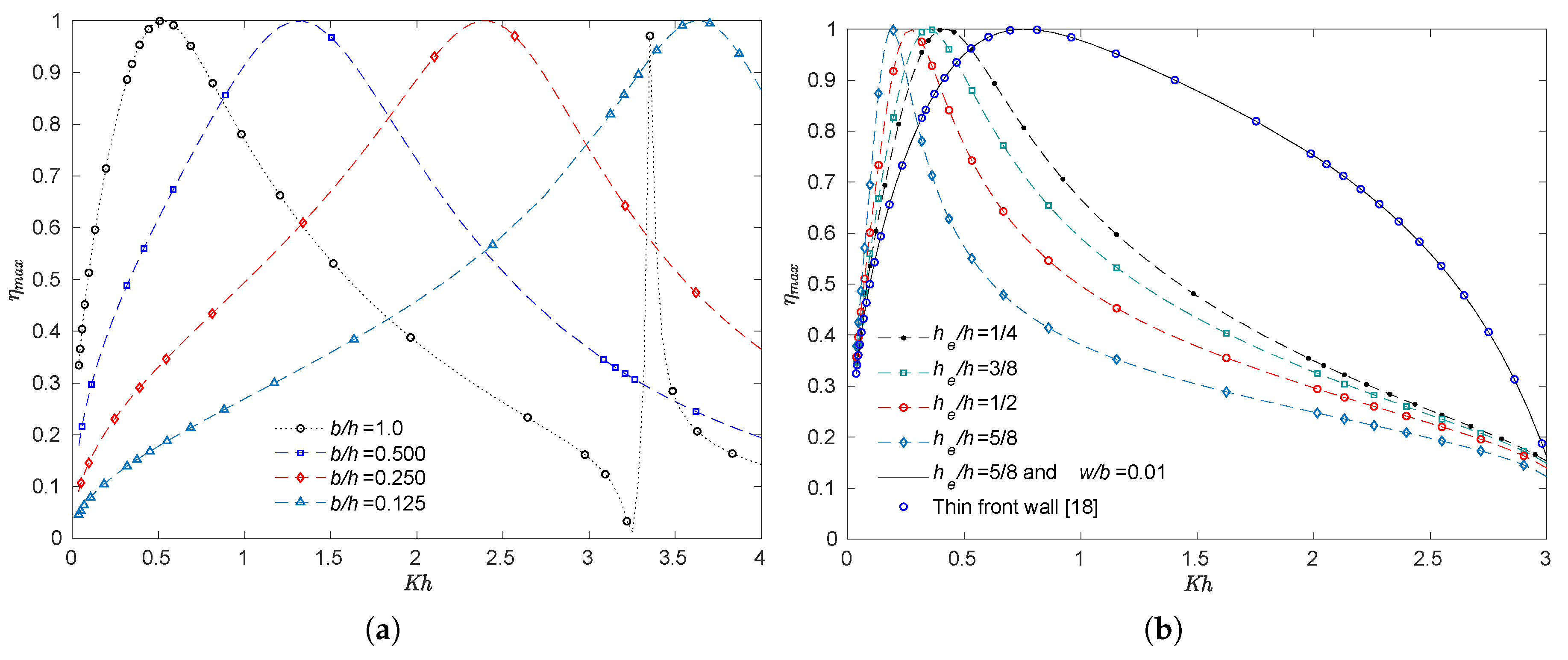
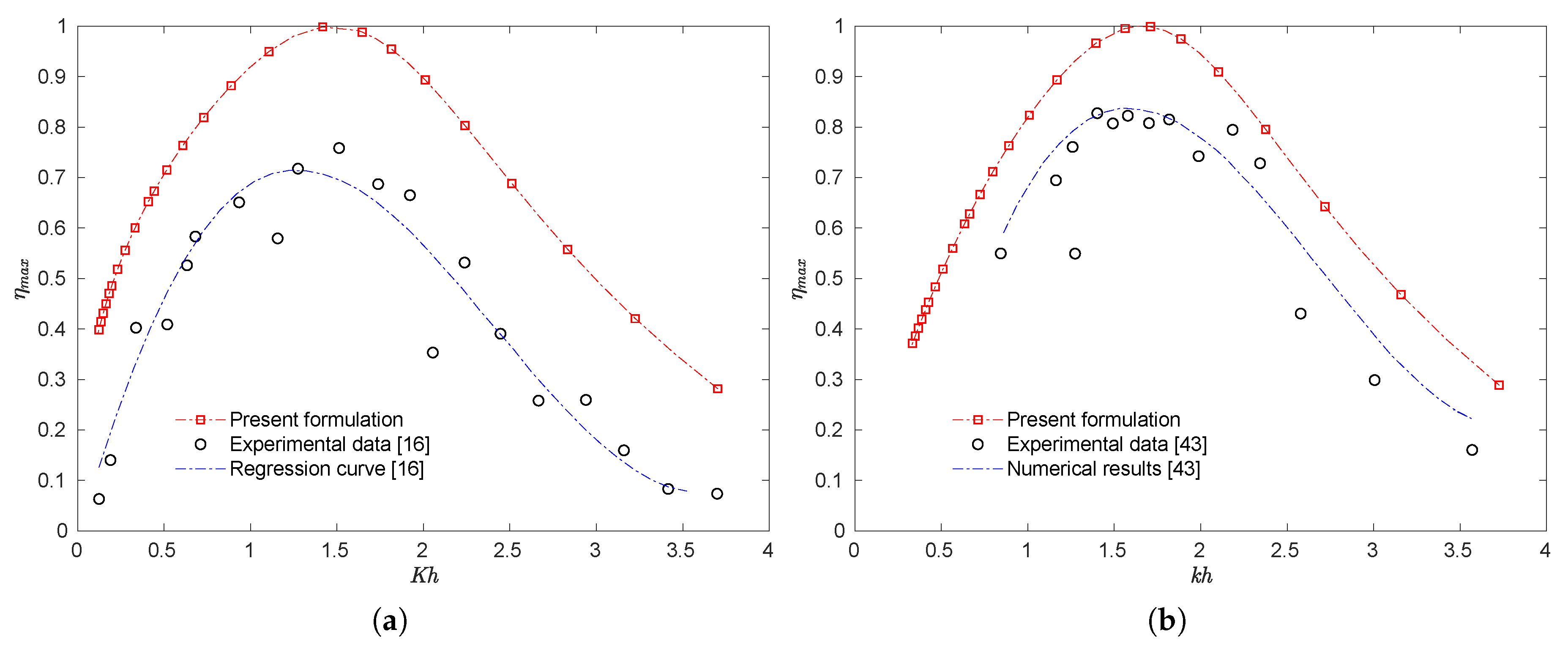
5. Results and Discussion

In this section, numerical results based on the BEM discussed in the previous section are presented. First, by considering a thick front wall and ignoring the influence of the air compressibility (i.e., $\varrho =0$), the effect of the chamber configuration on the hydrodynamic efficiency, radiation susceptance and radiation conductance coefficients is analyzed. Then, based on the physical dimensions of a single chamber of the MWEP, the effects of three different bottom profiles and the air compressibility on the efficiency are studied. It should be mentioned here that in order to minimize the effect of local disturbances at the far-field boundary, for the boundary discretization the distance between the front wall and the far-field boundary was considered to be 4 times the water depth h.

On the other hand, before performing the rest of the numerical calculations, a convergence analysis was carried out. In

Table 1. Values of hydrodynamic efficiency ${\eta }_{max}$, radiation susceptance coefficient $\mu$ and radiation conductance coefficient $\nu$ computed for different number of nodes N with $h_a/h=0.125$, $b/h=1.0$ and $w/b=0.5$.

N	$\mathit{K}\mathit{h}=$ 3.8329			$\mathit{K}\mathit{h}=$ 2.2657			$\mathit{K}\mathit{h}=$ 1.2054			$\mathit{K}\mathit{h}=$ 0.5074
	$\mathbf{\eta }$	$\mathit{\mu }$	$\mathit{\nu }$	$\mathit{\eta }$	$\mathit{\mu }$	$\mathit{\nu }$	$\mathit{\eta }$	$\mathit{\mu }$	$\mathit{\nu }$	$\mathit{\eta }$	$\mathit{\mu }$	$\mathit{\nu }$
560	0.2808	−0.2926	0.0484	0.4335	−0.3595	0.1035	0.8621	−0.6287	0.7299	0.9425	0.6507	1.2787
480	0.2814	−0.2940	0.0488	0.4337	−0.3598	0.1037	0.8622	−0.6295	0.7312	0.9425	0.6519	1.2806
400	0.2822	−0.2957	0.0492	0.4340	−0.3602	0.1039	0.8624	−0.6305	0.7329	0.9424	0.6534	1.2830
328	0.2833	−0.2982	0.0499	0.4343	−0.3608	0.1042	0.8626	−0.6318	0.7352	0.9423	0.6556	1.2861
256	0.2848	−0.3018	0.0508	0.4349	−0.3616	0.1046	0.8629	−0.6338	0.7386	0.9422	0.6587	1.2906
200	0.2856	−0.3071	0.0519	0.4370	−0.3644	0.1061	0.8636	−0.6373	0.7451	0.9418	0.6649	1.2978

, the results of the hydrodynamic efficiency $\eta$, radiation susceptance $\mu$ and radiation conductance $\nu$ for four different $Kh$ values are given. It is observed that around 480 nodes (240 quadratic elements) are enough to ensure convergence of the numerical results within three decimal places and also to avoid numerical instabilities that arise when the front wall thickness w tends to zero. Therefore, in the present calculations, all the BVPs are discretized through 480 nodes.

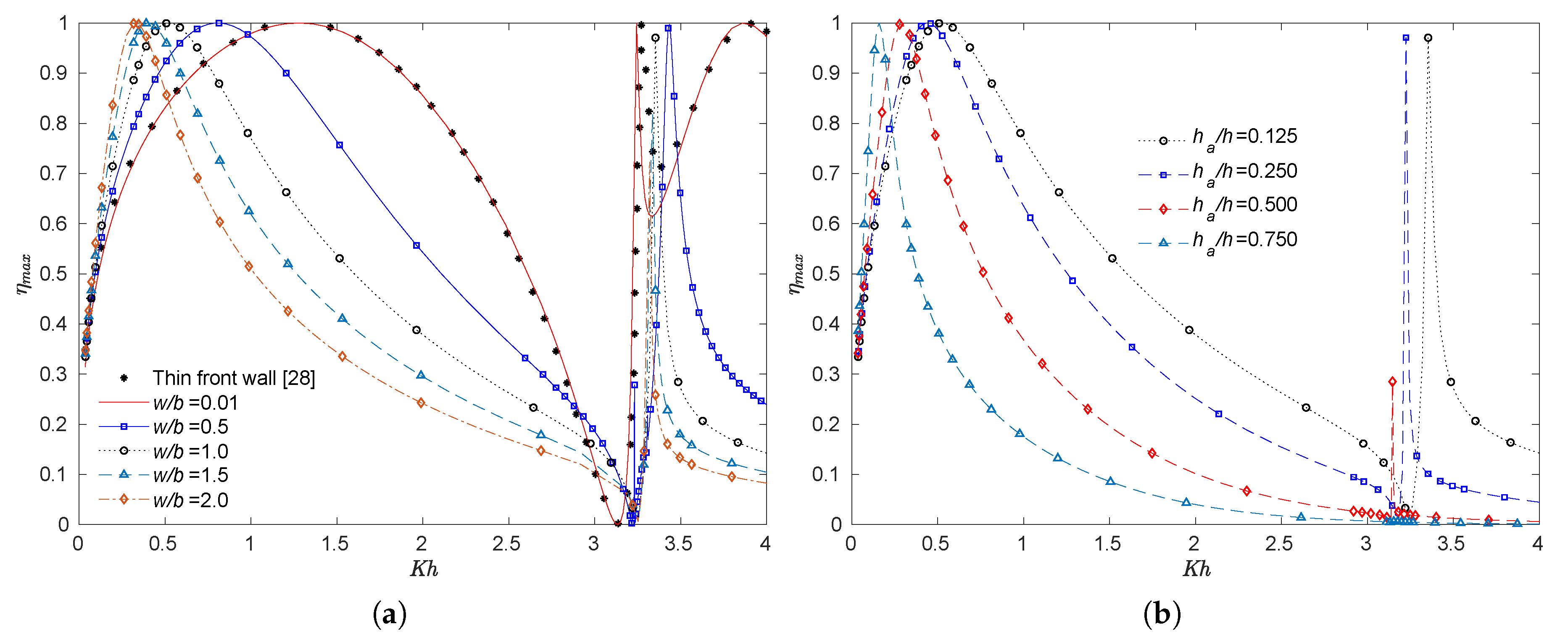
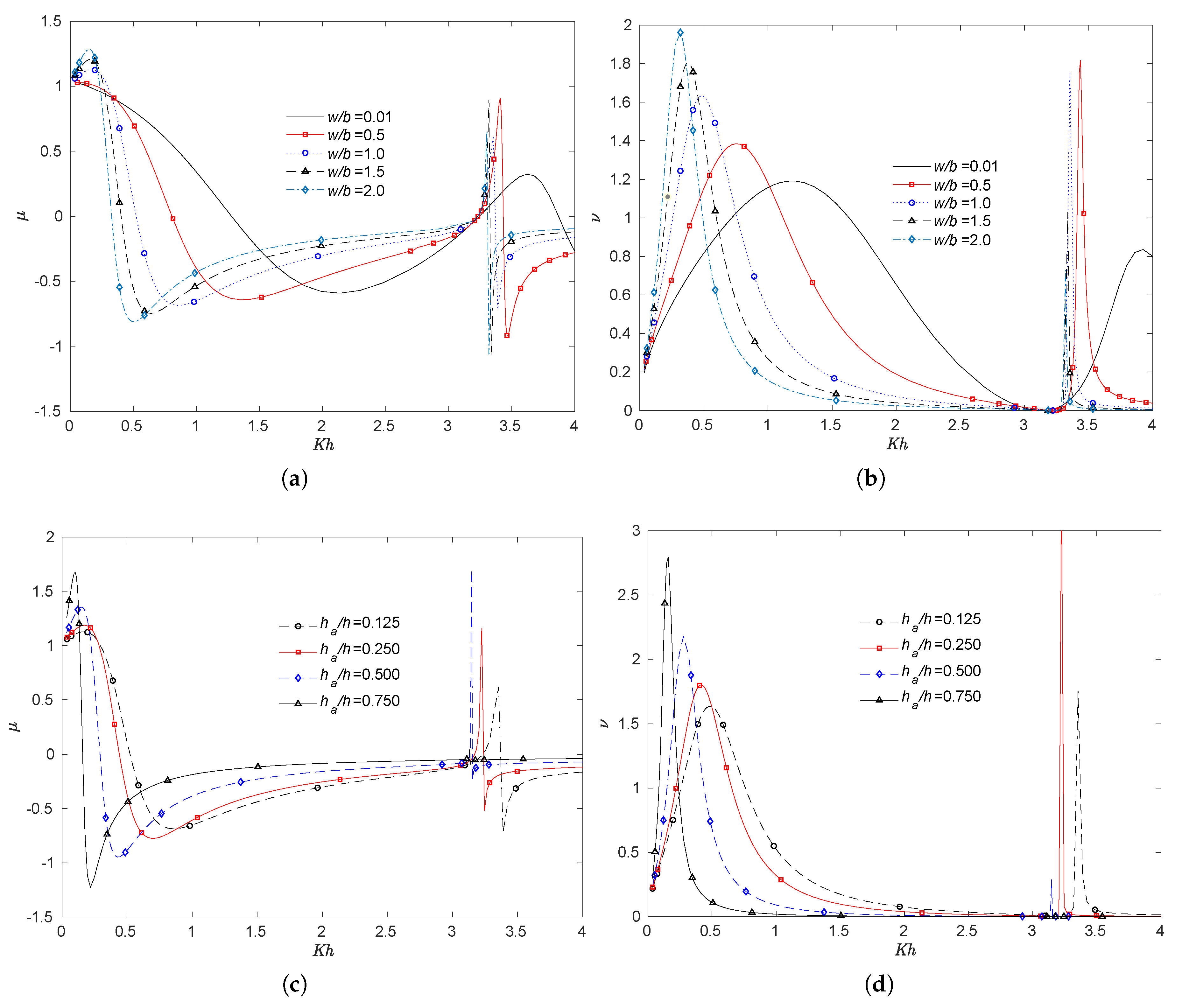
5.1. Front Wall Thickness

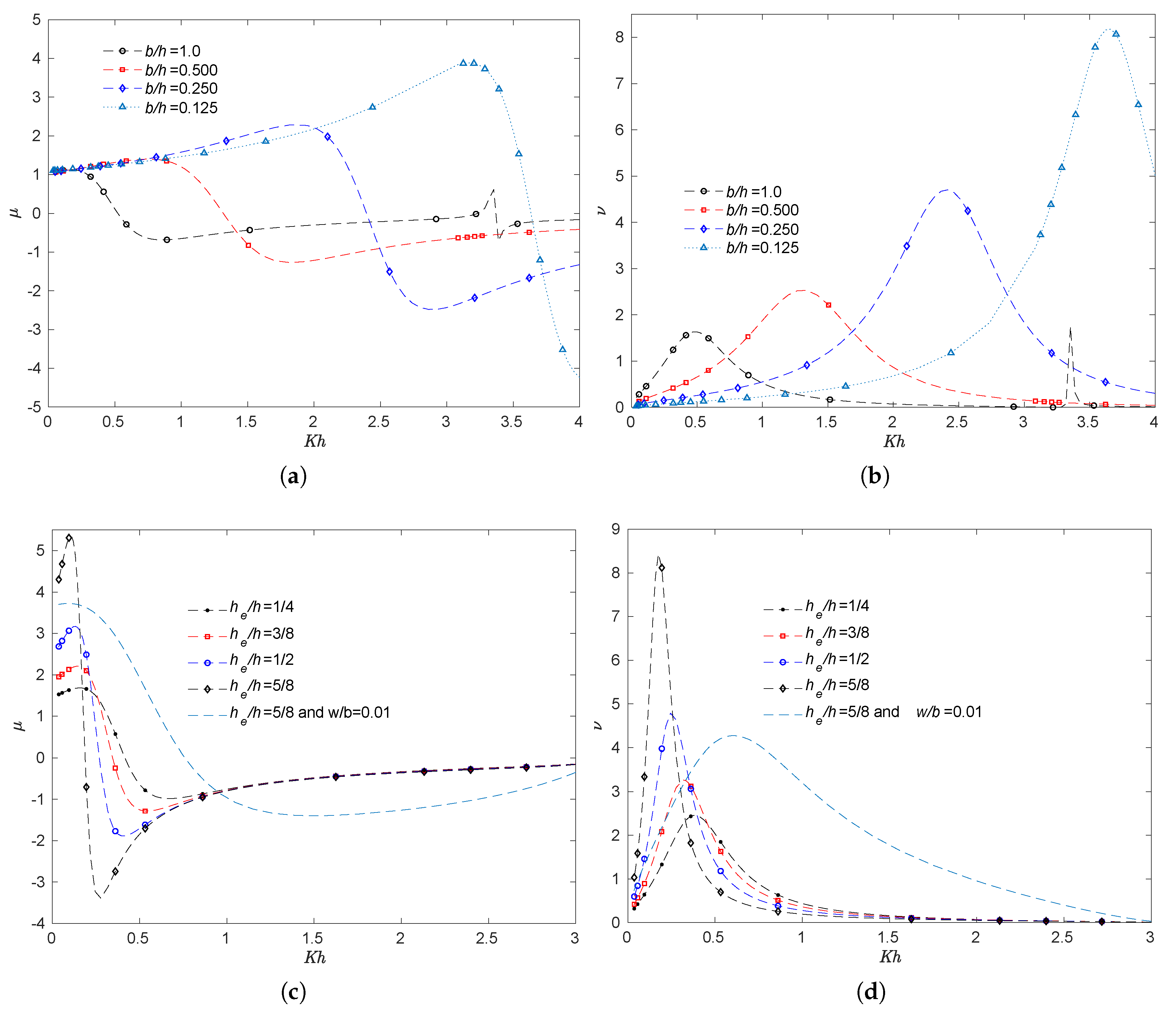
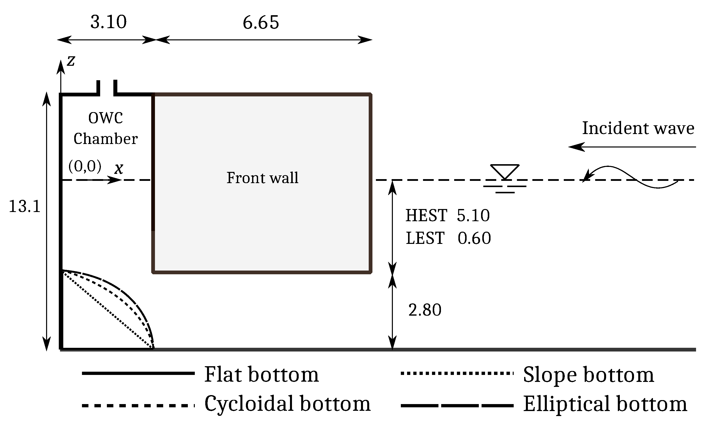
To validate the numerical method described here, the numerical results for the limiting case of Evans and Porter [28] were used. In the case of $h_a/h=0.125$, $b/h=1$, while w and $h_e$ tending to zero, the efficiency obtained by the present formulation was compared with the corresponding results of [28] for an OWC device with a horizontal topography, as shown in Figure 6a. The circles in Figure 6a depict the results of [28], whereas the line represents the results calculated by the present method. It can be seen that both results are in good agreement.

The numerical results of the efficiency ${\eta }_{max}$ versus $Kh$ for different thickness ratios $w/b(=2.0,1.5,1.0,0.5,\mathrm{and}0.01)$ in a flat bottom (without considering $h_e$) are shown in Figure 6a. In this figure, it is seen that by increasing the thickness of the front barrier, the bandwidth of the efficiency curves is reduced and their first peak frequency value is shifted to lower values of the non-dimensional frequency $Kh$. This reduction in the efficiency is explained by the fact that the energy transfer due to the wave motion over small periods is reduced when the front barriers are greater in thickness. However, in a real scenario, during severe storm events, or during times of high water levels, the front barrier is subjected to high loads, due to direct wave action [36,37,38,39], and a slender front wall cannot offer protection to the whole system, as occurred at the MWEP [12]. Therefore, special consideration should be given to this structural aspect.

On the other hand, Figure 6b shows the effect on efficiency of different submergance ratios $h_a/h(=0.125,0.250,0.500,\mathrm{and}0.750)$, together with a front barrier of the same thickness as the OWC chamber (i.e., $w/b=1.0$). In this figure, it is observed that the effective area of efficiency, under the curve, and the magnitude of the first natural frequency, both increase when the front wall $h_a/h$ decreases. Nevertheless, for a relatively small $h_a/h$, and considering that changes in water depth due to tidal variations and extreme waves may take place, a small draft may mean that the trough of a wave propagates below the front wall. This should be considered at the design stage, since in this situation the pressure within the chamber would be equivalent to the atmospheric pressure, causing the power available inside the OWC device to be zero and thus decreasing the efficiency.

The variation of the radiation susceptance and radiation conductance coefficients versus $Kh$ when $h_a/h=0.125$ and $b/h=1.0$ for different values of $w/b(=2.0,1.5,1.0,0.5,\mathrm{and}0.01)$ is shown in Figure 7a,b, respectively. In Figure 7a it is observed that the frequencies for which $\mu$ is zero are related to the peaks of maximum efficiency shown in Figure 6a, which is also evident from the maximum efficiency Equation (27). Figure 7a also shows that when the thickness ratio $w/b$ increases, the range of the non-dimensional frequency $Kh$ for which $\mu$ is negative also increases. As previously mentioned, the radiation susceptance $\mu$ is related to $\tilde{A}$ which is analogous to the added mass of the forced oscillation of a rigid body system. In this sense, the above-mentioned negative values in $\mu$ are may be due to the relevance of the free-surface effects of the internal free surface enclosed by the rigid wall and the surface-piercing front barrier. Negative values in the added mass are a common phenomenon in the theory of submerged and floating moving bodies in a fluid, such as when one or more elements of a structure enclose a portion of the free surface or two-dimensional cylinders are close to the free surface [40,41]. Furthermore, as demonstrated by Falnes [42], negative added mass occurs when an oscillating body produces a water motion where the associated potential energy is greater than the associated kinetic energy.

Figure 7b shows that the peaks in the radiation conductance $\nu$ are associated with those observed in Figure 6a. Together with Figure 7a, this shows that by increasing the radiation conductance coefficient $\nu$, with respect to the radiation susceptance coefficient $\mu$, an increase in the power extraction capacity can be attained. In this sense, the radiation conductance coefficient $\nu$ indicates the degree to which the system absorbs energy at different frequencies.

Figure 7c,d show the numerical results of the radiation susceptance and radiation conductance coefficients, respectively, versus $Kh$ with $w/b=1.0$, $b/h=1.0$ and for different submergance ratios $h_a/h(=0.125,0.250,0.500,\mathrm{and}0.750)$. In Figure 7c it is observed that by increasing the front wall draft $h_a$ with respect to h, the value of $Kh$ for which $\mu$ first become zero decreases, which is associated with the first resonance frequency inside the chamber, while the range of $Kh$ for negative values of $\mu$ increases. On the other hand, Figure 7d shows that a larger draft decreases the frequency at which this resonance occurs. It can also be observed that the peak resonance become more prominent the further the barrier is submerged. With a large draft, conditions are similar to those in a closed tank with parallel sides, where a second resonance mechanism occurs when the incident wave frequency is such that the fluid inside the chamber is excited into an antisymmetric sloshing mode [28]. In this case, the sloshing frequencies occur at values of the dimensionless wave number $kb=n\pi$, with n being the sloshing mode. For the case presented in Figure 7d, it is observed that the second peaks in $\nu$ due to the first sloshing frequency take place close to $Kh\approx \pi$.

Figure 8a plots the numerical results of the efficiency ${\eta }_{max}$ versus $Kh$ for various wall to front barrier spacing ratios $b/h(=1.0,0.5,0.25,\mathrm{and}0.125)$ with $h_a/h=0.125$ and $w/b=1.0$ with in a flat bottom. As reported by [19,28], large motions inside the chamber occur when the fluid between the front barrier and the back wall is excited by the incident wave into a resonant piston-like motion inside the OWC. An estimation of this natural frequency of oscillation can be obtained for small values of $b/h$ and so the water contained between the walls can be regarded as a solid body. By employing simple hydrostatic modelling gives that the expected resonance occurs at $Kh\approx h/h_a$. In the present case, this resonance would occur at $Kh=8$, which is seemed to be approached for smaller values of $b/h$. On the other hand, for a longer chamber, the frequency at which this resonance occurs is smaller. Physically, this is due to the fact that by increasing the length of the device, the horizontal distance a typical fluid particle must travel during a period of motion increases. This can also be obtained in the vertical direction by increasing the draft of the front wall. As a consequence, a decrease in the value of $Kh$ at which resonance occurs is caused, and since an increase in $b/h$ allows more local fluid motion inside the chamber, this leads to a breakdown in the solid-body model of resonance, and the amplitude of oscillation decreases.

Figure 8b illustrates the condition when a step, as long as the front wall, is placed below the latter with $h_a/h=0.125$, $b/h=1.0$ and $w/b=1.0$. First, a comparison of the present formulation with the limiting case of Şentürk and Özdamar [18] of an OWC device with a gap in its fully submerged thin front wall, together with the nondimensional parameters $h_a/h=0.125$, $h_e/h=0.625$, $b/h=1.0$ and $w/b=0.01$, is shown in Figure 8b. It can be seen that both results agree very well. Then, it can be observed that the smaller the distance between the front wall and the step, the lower the magnitude of the non-dimensional frequency $Kh$ at which resonance occurs. This is similar to the trend observed when the draft of the front wall is increased without considering the step, Figure 6b. A larger gap leads to a wider range of frequency bandwidth as it increases the transference of energy due to wave motion.

The numerical results for the radiation susceptance and radiation conductance coefficients versus $Kh$ when $h_a/h=0.125$ and $w/b=1.0$ for different values of $b/h(=1.0,0.5,0.25,\mathrm{and}0.125)$ are shown in Figure 9a,b, respectively. In Figure 9a, it is observed that when the wall to front barrier spacing is sufficiently small, compared to the depth h, the range of the non-dimensional frequency $Kh$ for which the radiation susceptance is negative decreases. Thus, when a small draft is considered, the $b/h$ ratio is important for the occurrence of negative values of the radiation susceptance coefficient. On the other hand, Figure 9b shows that when the length of chamber b increases with respect to the depth h, the radiation conductance coefficient peaks are maximum for longer periods. Consequently, since $\nu$ is a measure of the transfer of energy into the system, it may be beneficial to design the chamber length of the OWC device so that the range of frequency bandwidth in the radiation conductance coincides with the most occurring wave period of a particular location and thus exploit the available wave energy as much as possible.

Figure 9c,d show the radiation susceptance and radiation conductance coefficients, respectively, versus $Kh$ for various step to bottom ratios $h_e/h$ with $h_a/h=0.125$, $b/h=1.0$ and $w/b=1.0$. On one hand, Figure 9c shows that the variation from positive to negative in the radiation susceptance increases when the vertical spacing between the step and the front wall decreases. On the other hand, Figure 9d shows an increasing and narrowing peak for the radiation conductance coefficient, as the gap is reduced, decreasing the magnitude of the resonance frequency.

Figure 10a,b show a comparison of the present formulation with the experimental results obtained by Thomas et al. [16] and Wang et al. [43], respectively. First, in the case of a thick front wall considered by Thomas et al. [16], the OWC dimensions employed in the calculations are $h=$ 0.92 m, $b=$ 0.64 m $h_a=$ 0.15 m and $w=$ 0.08 m, while in the case of comparison with Wang et al. [43], the dimensions are $h=$ 0.80 m, $b=$ 0.55 m $h_a=$ 0.14 m and $w=$ 0.04 m. From Figure 10a,b, it is observed that by comparing the maximum theoretical efficiency and the experimental efficiency, the discrepancy is significant. The numerical solutions overpredict the hydrodynamic efficiency since it neglects the wave nonlinearity and the viscous dissipation, but the resonant frequencies and the shapes of the hydrodynamic efficiency curves predicted by the present numerical method agree well with each experiment [20,22]. It should be pointed out that the present formulation is based on the assumption of an ideal fluid and, therefore, viscous effects and flow separation due to the front wall are apparently the main cause of difference between the experimental and numerical results. Furthermore, another factor contributing to this discrepancy may be attributed to the rate of energy extraction modelled by the PTO system and the energy loss through it by viscous dissipation during the experiments.

In this sense, it is worth mentioning that ${\eta }_{max}=1$ theoretically means that the OWC device effectively captures all the incident wave energy, a condition that in practice is not feasible, due to the radiated wave generated by the oscillatory motion of the internal free surface, the scattering waves by the device and various viscous damping previously mentioned [20]. Thus, in a real scenario, a value of ${\eta }_{max}=$ 1 could never be achieved because of the energy loss through viscous dissipation as the fluid flow interacts with the chamber geometry and the PTO modelling. It should be mentioned that the effect of vortex and flow separation, which occur near the front wall, can be simulated well by introducing an artificial viscous damping term to the dynamic free surface boundary condition inside the OWC chamber and thus, to account for the energy loss due to vortex shedding and flow separation as previously reported by [20,22,43,44,45].

5.2. Bottom Profile

In this subsection, an analysis is made, based on the physical dimensions of the MWEP and on the highest and lowest tidal levels, Figure 11. The influence of different bottom profiles, the linear turbine damping and the linearized air compressibility inside the chamber on the hydrodynamic efficiency are evaluated. However, it should be noted that in this study the effect of the non-linear phenomena that occur in the interaction between the waves, the OWC device and the trapped air inside the chamber, such as viscous flow separation, turbulence, wave breaking and thermodynamic processes, are not taken into account. These aspects may play an important role in the performance of the OWC when variations in the bottom chamber are considered.

The varying bottom profiles proposed are defined in the interval 0 $\le x\le b$ and given by:

$$z=-h\left(x\right)=\left\{\begin{array}{cc}\left(\frac{h_a-h}{b}\right)x-h_a,\hfill & \mathrm{Sloped}\mathrm{bottom},\hfill \\ \left(\frac{h-h_a}{b}\right)\sqrt{b^2-x^2}-h,\hfill & \mathrm{Elliptical}\mathrm{bottom},\hfill \end{array}\right.$$

(49)

while the cycloidal bottom is given by the parametric equation

$$x\left(\widehat{\theta }\right)=\widehat{r}\left(\widehat{\theta }+sin\widehat{\theta }-\pi \right)+b,$$

(50a)

$$z\left(\widehat{\theta }\right)=\widehat{r}\left(cos\widehat{\theta }+1\right)-h,$$

(50b)

with $0.56416\le \widehat{\theta }\le \pi$ and $\widehat{r}=1.51759$ m.

In Figure 12, the numerical results for 1:1 sloped bottom profile with different linear turbine damping coefficients, $\mathsf{\Lambda }$, are compared with the experimental results obtained by Ashlin et al. [21] for a wave steepness $H_w/\lambda$ varying from $0.0320$ to $0.0371$. Regarding the numerical results presented here, it is worth noting that these are independent of the wave height since linear wave theory was employed for the formulation of the BVP. In order to perform the calculations, the OWC dimensions are those used by Ashlin et al. [21] in their experiments; these are $h=0.500$ m, $h_a=0.200$ m, $b=0.300$ m, $w=0.012$ m, a chamber width of $l=0.471$ m and a distance from the internal free surface to the top of the chamber of $s=0.400$ m. In order to see better the agreement between the results, the least-squares method was applied to the experimental data presented by [21] to obtain a best-fit second-order polynomial curve. Figure 12 shows that the numerical solution and the experimental results of [21] are in good agreement for a linear turbine damping coefficient $\mathsf{\Lambda }=$ 5 × 10${}^{-4}$ m${}^4·$s/kg. However, it is observed that by comparing the maximum theoretical efficiency obtained from Equation (27) and the experimental efficiency, the discrepancy is high. Therefore, special attention should be paid to turbine damping, as well as non-linear effects, in order to make an adequate estimation of the power absorption of an OWC device.

Figure 13a–d show the numerical results of the maximum ${\eta }_{max}$ versus the incoming wave period T for the cases when the HEST and LEST take place and the linearized air compressibility is considered. The range of wave period used in these figures is related to mean wave periods reported by [8]. In Figure 13a,c the maximum efficiency was obtained from Equation (25) with $\varrho =0$, while in Figure 13b,d, the optimum value of the damping coefficient (${\mathsf{\Lambda }}_{opt}$), calculated from Equation (23), was employed to obtain the hydrodynamic efficiency by considering the linearized air compressibility inside the chamber. In all the figures it can be seen that the efficiency band shifts slightly to the right as the bottom of the chamber becomes steeper, generating a slightly higher efficiency for higher periods. Figure 13a,b show that for incoming wave periods of less than 8 s, the flat bottom inside the chamber gives maximum efficiency. As reported by [21], this is due to the higher reflection generated by the curved bottom, together with the energy reflection caused by the front and back walls of the OWC device, for shorter wavelengths. The cycloidal and elliptical bottoms decrease the efficiency because these profiles reduce the section of the entrance of fluid particles, obstructing the waves and leading to a decrease in the internal free surface oscillation which drives the air column. This consequently diminishes the output power. The natural frequency of the system is seen to alter slightly for the different bottom profile configurations. Figure 13c,d show the efficiency in the case of the lowest equinoctial spring tide. As expected, compared with the HEST, the period at which resonance takes place is reduced due to the lower front wall draft, $h_a=0.60$ m. Furthermore, as observed in Figure 6b, Figure 13c shows that the efficiency effective area under the curve increases with a shorter front wall draft. However, in the case of Mutriku, where significant wave heights of 4 m are common [8], this small draft increases the possibility that the wave trough propagates below the front wall, and thus reduces efficiency. Regarding the effect of the volume of air inside the chamber, compared with Figure 13b, Figure 13d shows that efficiency is significantly reduced when the air volume is larger. Comparing Figure 13d to Figure 13c shows that the period at which resonance occurs is independent of the damping condition and is mostly determined by the natural frequency of the water column.

6. Conclusions

The effects of the chamber configuration of an OWC device on efficiency were numerically analyzed, using the BEM, employing quadratic elements. Comparisons were made of these numerical results with theoretical limiting cases obtained by Evans and Porter [28] and Şentürk and Özdamar [18] for a thin front wall and very good agreement was achieved. Numerical estimates for the hydrodynamic efficiency and the radiation susceptance and radiation conductance coefficients were then obtained for different physical configurations. Experimental results reported by Thomas et al. [16] and Wang et al. [43] were compared with those obtained by the present formulation; resonance frequencies and shapes of the hydrodynamic efficiency curves were found to be in good agreement. The main conclusions drawn from this study are as follows:

• By increasing the thickness of the front barrier, the bandwidth on the efficiency curves is reduced. This reduction in efficiency could be related to the fact that the transfer of energy from the incoming wave to the internal free surface, due to the orbital wave motion, is reduced for short wave periods when the front barrier is thicker.
• For a thick front barrier, a further reduction in the efficiency effective area under the curve is obtained when the front wall draft is increased.
• When the OWC chamber length-water depth ratio $b/h$ is decreased, the period of maximum hydrodynamic efficiency is shorter. Consequently, an OWC chamber in which the range of frequency bandwidth in ${\eta }_{max}$ coincides with the predominant wave period of a particular location, will mean the available wave power will be made better use of.
• It was observed that the incorporation of a step below the front wall reduces the bandwidth on the efficiency. This step gives a similar effect as that observed when the draft of the front wall is increased in an OWC with a completely flat bottom.
• It was also observed that when the wall to front barrier spacing is sufficiently small, compared to the depth, the range of the non-dimensional frequency $Kh$, for which the radiation susceptance coefficient is negative, is significantly reduced.
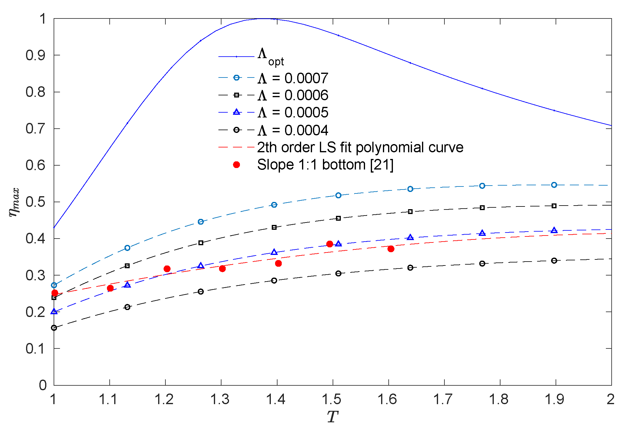
• By comparing the maximum theoretical efficiency with the experimental efficiency reported by Ashlin et al. [21] for a wave steepness $H/\lambda$ varying from $0.0320$ to $0.0371$, the discrepancy is seen to be high. Therefore, special attention should be paid to turbine damping, as well as to non-linear effects, in order to make an adequate estimation of the power absorption of an OWC.
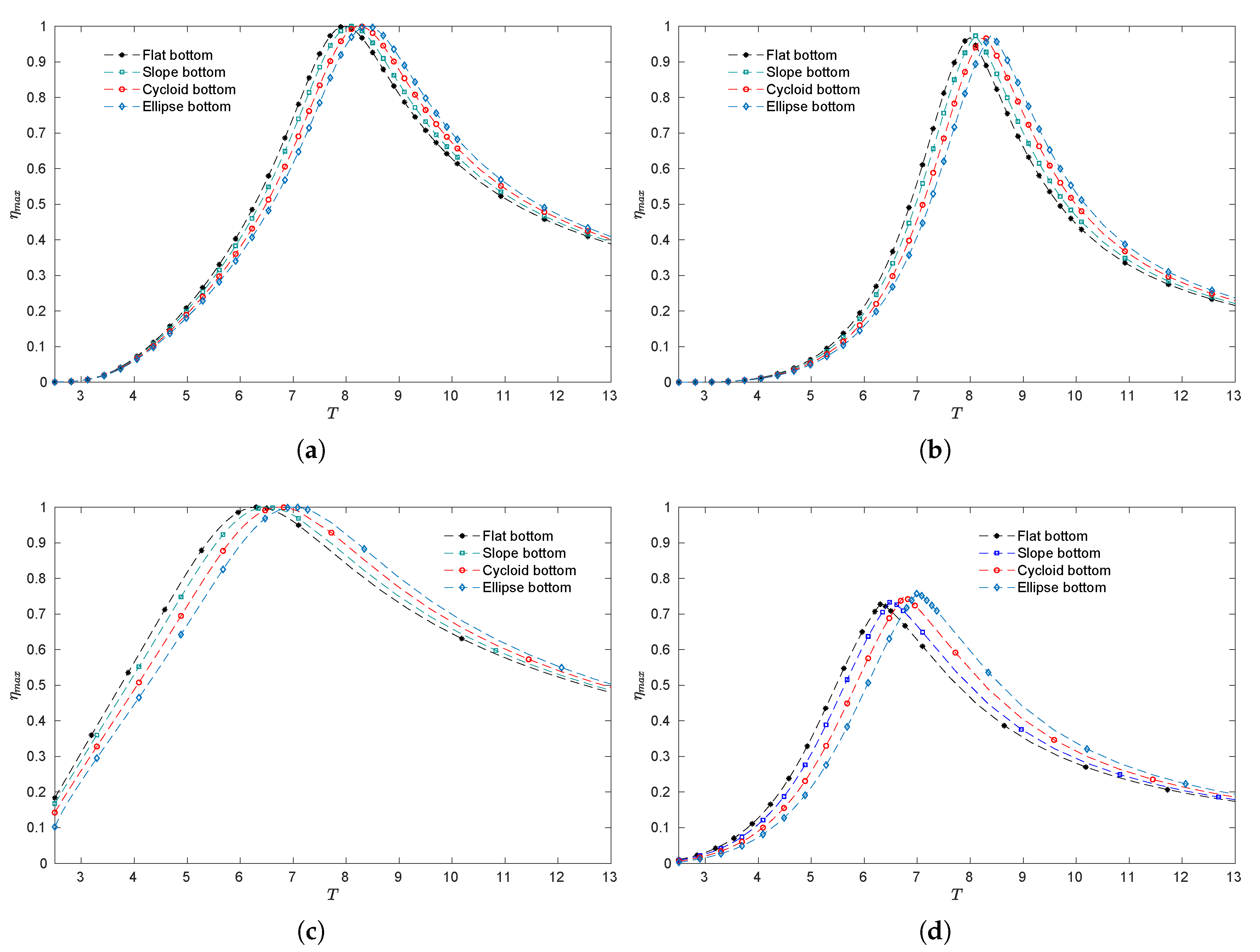
• When sloped, cycloidal or elliptical bottom profiles in a chamber of the MWEP were considered, it was seen that the efficiency band slightly shifts to longer periods, as the bottom of the chamber becomes steeper, generating slightly higher efficiency for longer wavelengths.
• For small periods, it was found that compared with the flat bottom, the sloped, cycloidal and elliptical bottoms diminish the hydrodynamic efficiency. This is due to the reduction of the part of the chamber entrance for the fluid particles, obstructing the waves and leading to a decrease in the internal free surface oscillation which drives the air column.
• It was observed that in the case of LEST in the MWEP, the efficiency band becomes wider as the draft is reduced. However, when the air volume inside the chamber is greater, the efficiency is significantly reduced.
• By comparing the different bottom profiles, it was found that the period in which resonance occurs is almost independent of the bottom geometrical configuration and it is mostly determined by the natural frequency of the water column.

This paper is only a numerical investigation on the hydrodynamic performance of an OWC device based on the linear wave theory. Experimental investigations that include the non-linearities on the air compressibility and the turbine damping should be carried out in the future. Finally, it is hoped that the results of this study may provide valuable information for the clean and efficient harnessing of marine renewable energy.

References

1. Izquierdo, U.; Adolfo Esteban, G.; Blanco, J.M.; Albaina, I.; Peña, A. Experimental validation of a CFD model using a narrow wave flume. Appl. Ocean Res. 2019, 86, 1–12. [Google Scholar] [CrossRef]
2. Ahamed, R.; McKee, K.; Howard, I. Advancements of wave energy converters based on power take off (PTO) systems: A review. Ocean Eng. 2020, 204, 107248. [Google Scholar] [CrossRef]
3. Falcão, A.F.O.; Henriques, J.C.C. Oscillating-water-column wave energy converters and air turbines: A review. Renew. Energy 2016, 85, 1391–1424. [Google Scholar] [CrossRef]
4. Vicinanza, D.; Di Lauro, E.; Contestabile, P.; Gisonni, C.; Lara, J.L.; Losada, I.J. Review of Innovative Harbor Breakwaters for Wave-Energy Conversion. J. Waterway Port Coast. Ocean Eng. 2019, 145, 03119001. [Google Scholar] [CrossRef]
5. Polinder, H.; Scuotto, M. Wave energy converters and their impact on power systems. In Proceedings of the International Conference on Future Power Systems, Amsterdam, The Netherlands, 16–18 November 2005. [Google Scholar]
6. Torre-Enciso, Y.; Ortubia, I.; López De Aguileta, L.I.; Marqués, J. Mutriku Wave Power Plant: From the Thinking out to the Reality. In Proceedings of the 8th European Wave and Tidal Energy Conference (EWTEC), Uppsala, Sweden, 7–10 September 2009. [Google Scholar]
7. Garrido, A.J.; Otaola, E.; Garrido, I.; Lekube, J.; Maseda, F.J.; Liria, P.; Mader, J. Mathematical Modeling of Oscillating Water Columns Wave-Structure Interaction in Ocean Energy Plants. Math. Prob. Eng. 2015, 2015, 727982. [Google Scholar] [CrossRef] [Green Version]
8. Ibarra-Berastegi, G.; Sáenz, J.; Ulazia, A.; Serras, P.; Esnaola, G.; Garcia-Soto, C. Electricity production, capacity factor, and plant efficiency index at the Mutriku wave farm (2014–2016). Ocean Eng. 2018, 147, 20–29. [Google Scholar] [CrossRef] [Green Version]
9. Google Maps 2020. Available online: https://www.google.es/maps (accessed on 10 July 2020).
10. GeoEuskadi, Infraestructura de Datos Espaciales (IDE) de Euskadi. Available online: http://www.geo.euskadi.eus (accessed on 10 July 2020).
11. Ente Vasco de la Energía. Available online: http://www.eve.es (accessed on 15 August 2020).
12. Medina-Lopez, E.; Allsop, W.; Dimakopoulos, A.; Bruce, T. Conjectures on the Failure of the OWC Breakwater at Mutriku. In Proceedings of the Coastal Structures and Solutions to Coastal Disasters Joint Conference, Boston, MA, USA, 9–11 September 2015. [Google Scholar]
13. Heath, T.V. A review of oscillating water columns. Philos. Trans. R. Soc. A 2012, 370, 235–245. [Google Scholar] [CrossRef] [Green Version]
14. Delmonte, N.; Barater, D.; Giuliani, F.; Cova, P.; Buticchi, G. Review of Oscillating Water Column Converters. IEEE Trans. Ind. Appl. 2016, 52, 1698–1710. [Google Scholar] [CrossRef]
15. Wang, D.J.; Katory, M.; Li, Y.S. Analytical and experimental investigation on the hydrodynamic performance of onshore wave-power devices. Ocean Eng. 2002, 29, 871–885. [Google Scholar] [CrossRef]
16. Morris-Thomas, M.T.; Irvin, R.J.; Thiagarajan, K.P. An Investigation Into the Hydrodynamic Efficiency of an Oscillating Water Column. J. Offshore Mech. Arct. 2006, 129, 273–278. [Google Scholar] [CrossRef]
17. Martins-rivas, H.; Mei, C.C. Wave power extraction from an oscillating water column along a straight coast. Ocean Eng. 2009, 36, 426–433. [Google Scholar] [CrossRef]
18. Şentürk, U.; Özdamar, A. Wave energy extraction by an oscillating water column with a gap on the fully submerged front wall. Appl. Ocean Res. 2012, 37, 174–182. [Google Scholar] [CrossRef]
19. Rezanejad, K.; Bhattacharjee, J.; Guedes Soares, C. Stepped sea bottom effects on the efficiency of nearshore oscillating water column device. Ocean Eng. 2013, 70, 25–38. [Google Scholar] [CrossRef]
20. Ning, D.Z.; Shi, J.; Zou, Q.P.; Teng, B. Investigation of hydrodynamic performance of an OWC (oscillating water column) wave energy device using a fully nonlinear HOBEM (higher-order boundary element method). Energy 2015, 83, 177–188. [Google Scholar] [CrossRef]
21. John Ashlin, S.; Sundar, V.; Sannasiraj, S.A. Effects of bottom profile of an oscillating water column device on its hydrodynamic characteristics. Renew. Energy 2016, 96, 341–353. [Google Scholar] [CrossRef]
22. Ning, D.Z.; Wang, R.Q.; Zou, Q.P.; Teng, B. An experimental investigation of hydrodynamics of a fixed OWC Wave Energy Converter. Appl. Energy 2016, 168, 636–648. [Google Scholar] [CrossRef]
23. Zheng, S.; Zhang, Y.; Iglesias, G. Coast/breakwater-integrated OWC: A theoretical model. Mar. Struct. 2019, 66, 121–135. [Google Scholar] [CrossRef]
24. Zheng, S.; Alessandro, A.; Zhang, Y.; Greaves, D.; Miles, J.; Iglesias, G. Wave power extraction from multiple oscillating water columns along a straight coast. J. Fluid Mech. 2019, 878, 445–480. [Google Scholar] [CrossRef]
25. Zheng, S.; Zhu, G.; Simmonds, D.; Greaves, D.; Iglesias, G. Wave power extraction from a tubular structure integrated oscillating water column. Renew. Energy 2020, 150, 342–355. [Google Scholar] [CrossRef]
26. Koley, S.; Trivedi, K. Mathematical modeling of oscillating water column wave energy converter devices over the undulated sea bed. Eng. Anal. Bound. Elem. 2020, 117, 26–40. [Google Scholar] [CrossRef]
27. Belibassakis, K.; Magkouris, A.; Rusu, E. A BEM for the Hydrodynamic Analysis of Oscillating Water Column Systems in Variable Bathymetry. Energies 2020, 13, 3403. [Google Scholar] [CrossRef]
28. Evans, D.V.; Porter, R. Hydrodynamic characteristics of an oscillating water column device. Appl. Ocean Res. 1995, 17, 155–164. [Google Scholar] [CrossRef]
29. Evans, D.V. Wave-power absorption by systems of oscillating surface pressure distributions. J. Fluid Mech. 1982, 114, 481–499. [Google Scholar] [CrossRef]
30. Rezanejad, K.; Guedes Soares, C.; López, I.; Carballo, R. Experimental and numerical investigation of the hydrodynamic performance of an oscillating water column wave energy converter. Renew. Energy 2017, 106, 1–16. [Google Scholar] [CrossRef]
31. Michele, S.; Renzi, E.; Perez-Collazo, C.; Greaves, D.; Iglesias, G. Power extraction in regular and random waves from an OWC in hybrid wind-wave energy systems. Ocean Eng. 2019, 191, 106519. [Google Scholar] [CrossRef]
32. Katsikadelis, J. Boundary Elements. Theory and Applications; Elsevier: Amsterdam, The Netherlands, 2002. [Google Scholar]
33. Dominguez, J. Boundary Elements in Dynamics; Computational Mechanics Publications: Southampton, UK, 1993. [Google Scholar]
34. Brebbia, C.A.; Dominguez, J. Boundary Elements: An Introductory Course; Computational Mechanics Publications: Southampton, UK, 1992. [Google Scholar]
35. Becker, A. The Boundary Element Method in Engineering: A Complete Course; McGraw-Hill Book Company: London, UK, 1992. [Google Scholar]
36. Viviano, A.; Naty, S.; Foti, E.; Bruce, T.; Allsop, W.; Vicinanza, D. Large-scale experiments on the behaviour of a generalised Oscillating Water Column under random waves. Renew. Energy 2016, 99, 875–887. [Google Scholar] [CrossRef] [Green Version]
37. Pawitan, K.A.; Dimakopoulos, A.S.; Vicinanza, D.; Allsop, W.; Bruce, T. A loading model for an OWC caisson based upon large-scale measurements. Coast. Eng. 2019, 145, 1–20. [Google Scholar] [CrossRef] [Green Version]
38. Viviano, A.; Musumeci, R.E.; Vicinanza, D.; Foti, E. Pressures induced by regular waves on a large scale OWC. Coast. Eng. 2019, 152, 103528. [Google Scholar] [CrossRef]
39. Pawitan, K.A.; Vicinanza, D.; Allsop, W.; Bruce, T. Front Wall and In-Chamber Impact Loads on a Breakwater-Integrated Oscillating Water Column. J. Waterway Port Coast. Ocean Eng. 2020, 146, 04020037. [Google Scholar] [CrossRef]
40. McIver, P.; Evans, D.V. The occurrence of negative added mass in free-surface problems involving submerged oscillating bodies. J. Eng. Math. 1984, 18, 7–22. [Google Scholar] [CrossRef]
41. McIver, M.; McIver, P. The added mass for two-dimensional floating structures. Wave Motion 2016, 64, 1–12. [Google Scholar] [CrossRef] [Green Version]
42. Falnes, J. Added-Mass Matrix and Energy Stored in the “Near Field”; Internal Report Division of Experimental Physics, University of Trondheim: Trondheim, Norway, 1983. [Google Scholar]
43. Wang, R.Q.; Ning, D.Z.; Zhang, C.W.; Zou, Q.P.; Liu, Z. Nonlinear and viscous effects on the hydrodynamic performance of a fixed OWC wave energy converter. Coast. Eng. 2018, 131, 42–50. [Google Scholar] [CrossRef]
44. Ning, D.Z.; Wang, R.Q.; Gou, Y.; Zhao, M.; Teng, B. Numerical and experimental investigation of wave dynamics on a land-fixed OWC device. Energy 2016, 115, 326–337. [Google Scholar] [CrossRef]
45. Wang, R.Q.; Ning, D.Z. Dynamic analysis of wave action on an OWC wave energy converter under the influence of viscosity. Renew. Energy 2020, 150, 578–588. [Google Scholar] [CrossRef]
Figure 1. Location and turbo-generators of the MWEP. (a) Location of the harbour at Mutriku (source: Google Maps [9]). (b) Bird’s eye view of Mutriku harbour and the OWC-breakwater system. (source: geoEuskadi [10]). (c) Mutriku Wells Turbo-generators (source: EVE [11]).
Jmse 08 00751 g001
Figure 2. Comparison between the original and the present-day design of the integrated breakwater-OWC system in Mutriku. (a) View of the MWEP in 2008 (Reproduced with permission from [6]). (b) Mutriku OWC (source: EVE [11]).
Jmse 08 00751 g002
Figure 3. Definition sketch of an OWC device with a thick front wall.
Jmse 08 00751 g003
Figure 4. Schematic diagram of the modeling of the boundary with quadratic elements.
Jmse 08 00751 g004
Figure 5. Boundary element discretization of the composite domain. (a) Separation of the BVP into three regions. (b) Discretization of the three regions.
Jmse 08 00751 g005
Figure 6. Hydrodynamic efficiency versus K h . (a) For various thickness ratios w / b with h a / h = 0.125 and b / h = 1.0 . (b) For different submergence ratios h a / h with w / b = 1.0 and b / h = 1.0 .
Jmse 08 00751 g006
Figure 7. The radiation susceptance and radiation conductance coefficients versus K h . (a) The radiation susceptance coefficient for various thickness ratios w / b with h a / h = 0.125 and b / h = 1.0 . (b) The radiation conductance coefficient for various thickness ratios w / b with h a / h = 0.125 and b / h = 1.0 . (c) The radiation susceptance coefficient for different submergance ratios h a / h with w / b = 1.0 and b / h = 1.0 . (d) The radiation conductance coefficient for different submergance ratios h a / h with w / b = 1.0 and b / h = 1.0 .
Jmse 08 00751 g007
Figure 8. Hydrodynamic efficiency versus K h . (a) For various wall to front barrier spacing ratios b / h with h a / h = 0.125 and w / b = 1.0 . (b) For various step to bottom ratios h e / h with h a / h = 0.125 , b / h = 1.0 and w / b = 1.0 .
Jmse 08 00751 g008
Figure 9. The radiation susceptance and radiation conductance coefficients versus K h . (a) The radiation susceptance coefficient for various wall to front barrier spacing ratios b / h with h a / h = 0.125 and w / b = 1.0 . (b) The radiation conductance coefficient for various wall to front barrier spacing ratios b / h with h a / h = 0.125 and w / b = 1.0 . (c) The radiation susceptance coefficient for various step to bottom ratios h e / h with h a / h = 0.125 , b / h = 1.0 and w / b = 1.0 . (d) The radiation conductance coefficient for various step to bottom ratios h e / h with h a / h = 0.125 , b / h = 1.0 and w / b = 1.0 .
Jmse 08 00751 g009
Figure 10. Hydrodynamic efficiency versus (a) K h and (b) k h . (a) Comparison with experimental results obtained by Thomas et al. [16] for a thick front wall. (b) Comparison with experimental and numerical results obtained by Wang et al. [43].
Jmse 08 00751 g010
Figure 11. Definition sketch of a single chamber in the Mutriku Wave Energy Plant (Dimensions in meters. Chamber width = 4.5 m; HEST = Highest equinoctial spring tide and LEST = Lowest equinoctial spring tide).
Jmse 08 00751 g011
Figure 12. Hydrodynamic efficiency versus period T for different values of linear turbine damping coefficient Λ , without considering the step.
Jmse 08 00751 g012
Figure 13. Hydrodynamic efficiency in the cases of HEST and LEST versus T for different bottom profiles. (a) Maximum efficiency versus T with ϱ = 0 for various bottom profiles with h = 7.90 , h a / h = 0.646 , b / h = 0.392 and w / b = 2.145 in the case of the HEST. (b) Maximum efficiency versus T for various bottom profiles with h = 7.90 , h a / h = 0.646 , b / h = 0.392 and w / b = 2.145 . in the case of the HEST. (c) Maximum efficiency versus T with ϱ = 0 for various bottom profiles with h = 3.40 , h a / h = 0.176 , b / h = 0.392 and w / b = 2.145 in the case of the LEST. (d) Maximum efficiency versus T for various bottom profiles with h = 3.40 , h a / h = 0.176 , b / h = 0.392 and w / b = 2.145 in the case of the LEST.
Jmse 08 00751 g013