UAV Photogrammetry and Ground Surveys as a Mapping Tool for Quickly Monitoring Shoreline and Beach Changes


Abstract
1. Introduction
2. Study Area
3. Data Availability
- DJI Matrice 600, 525 × 480 × 640 mm, max take-off weight 15.5 kg, with a max. payload of 5.5 kg and flight time of approximately 30 min, equipped with a DJI M600-X5 camera;
- DJI Spark, 143 × 143 × 55 mm, lightened to a weight less than 300g and flight time of approximately 16 min, equipped with a DJI FC 1102 camera.
4. Photogrammetric Analysis
5. PPK and NRTK GNSS Surveys
6. Empirical Accuracy Assessment of PPK and Photogrammetric Surveys
7. Results
8. Discussion and Conclusions
Supplementary Materials
Author Contributions
Funding
Acknowledgments
Conflicts of Interest
References
- Smith, A.W.S.; Jackson, L.A. The variability in width of the visible beach. Shore Beach 1992, 60, 7–15. [Google Scholar]
- Armaroli, C.; Ciavola, P.; Perini, L.; Lorito, S.; Valentini, A.; Masina, M. Critical storm thresholds for significant morphological changes and damage along the Emilia-Romagna coastline, Italy. Geomorphology 2012, 143–144, 34–51. [Google Scholar] [CrossRef]
- Cantasano, N.; Pellicone, G.; Ietto, F. Integrated coastal zone management in Italy: A gap between science and policy. J. Coast Conserv. 2017, 21, 317–325. [Google Scholar] [CrossRef]
- Ciavola, P.; Armaroli, C.; Chiggiato, J.; Valentini, A.; Deserti, M.; Perini, L.; Luciani, P. Impact of storms along the coastline of Emilia-Romagna: The morphological signature on the Ravenna coastline (Italy). J. Coast. Res. 2007, 540–544. [Google Scholar]
- Moore, L.J. Shoreline mapping techniques. J. Coast. Res. 2000, 16, 111–124. [Google Scholar] [CrossRef]
- Boak, E.; Turner, I.L. Shoreline definition and detection: A review. J. Coast. Res. 2005, 21, 688–703. [Google Scholar] [CrossRef]
- Michalowska, K.; Glowienka, E.; Pekala, A. Spatial-Temporal detection of changes on the southern coast of the Baltic sea based on multitemporal aerial photographs. In Proceedings of the International Archives of the Photogrammetry, Remote Sensing and Spatial Information Sciences—ISPRS Archives, Prague, Czech Republic, 12–19 July 2016; Volume 41, pp. 49–53. [Google Scholar] [CrossRef]
- Schwarzer, K.; Diesing, M.; Larson, M.; Niedermeyer, R.O.; Schumacher, W.; Furmanczyk, K. Coastline evolution at different time scales—Examples from the Pomeranian Bight, southern Baltic Sea. Mar. Geol. 2003, 194, 79–101. [Google Scholar] [CrossRef]
- Benassai, G.; Aucelli, P.; Budillon, G.; De Stefano, M.; Di Luccio, D.; Di Paola, G.; Montella, R.; Mucerino, L.; Sica, M.; Pennetta, M. Rip current evidence by hydrodynamic simulations, bathymetric surveys and UAV observation. Nat. Hazards Earth Syst. Sci. 2017, 17, 1493–1503. [Google Scholar] [CrossRef]
- Casella, E.; Rovere, A.; Pedroncini, A.; Stark, C.P.; Casella, M.; Ferrari, M.; Firpo, M. Drones as tools for monitoring beach topography changes in the Ligurian Sea (NW Mediterranean). Geo-Mar. Lett. 2016, 36, 151–163. [Google Scholar] [CrossRef]
- Duo, E.; Trembanis, A.C.; Dohner, S.; Grottoli, E.; Ciavola, P. Local-scale post-event assessments with GPS and UAV based quick-response surveys: A pilot case from the Emilia—Romagna (Italy). Coast. Nat. Hazards Earth Syst. Sci. 2018, 18, 2969–2989. [Google Scholar] [CrossRef]
- Giordan, D.; Notti, D.; Villa, A.; Zucca, F.; Calò, F.; Pepe, A.; Dutto, F.; Pari, P.; Baldo, M.; Allasia, P. Low cost, multiscale and multi-sensor application for flooded area mapping. Nat. Hazards Earth Syst. Sci. 2018, 18, 1493–1516. [Google Scholar] [CrossRef]
- Mancini, F.; Dubbini, M.; Gattelli, M.; Stecchi, F.; Fabbri, S.; Gabbianelli, G. Using Unmanned Aerial Vehicles (UAV) for High-Resolution Reconstruction of Topography: The Structure from Motion Approach on Coastal Environments. Remote Sens. 2013, 5, 6880–6898. [Google Scholar] [CrossRef]
- Turner, I.L.; Harley, M.D.; Drummond, C.D. UAVs for coastal surveying. Coast. Eng. 2016, 114, 19–24. [Google Scholar] [CrossRef]
- Van Puijenbroek, M.E.; Nolet, B.; de Groot, C.; Suomalainen, A.V.; Riksen, J.M.; Berendse, M.J.P.M.; Limpens, F.J. Exploring the contributions of vegetation and dune size to early dune development using unmanned aerial vehicle (UAV) imaging. Biogeosciences 2017, 14, 5533–5549. [Google Scholar] [CrossRef]
- Guariglia, A.; Buonamassa, A.; Losurdo, A.; Saladino, R.; Trivigno, M.L.; Zaccagnino, A.; Colangelo, A. A multisource approach for coastline mapping and identification of shoreline changes. Ann. Geophys. 2006, 49, 295–304. [Google Scholar] [CrossRef]
- Bazzichetto, M.; Malavasi, M.; Acosta, A.T.R.; Carranza, M.L. How does dune morphology shape coastal EC habitats occurrence? A remote sensing approach using airborne LiDAR on the Mediterranean coast. Ecol. Indic. 2016, 71, 618–626. [Google Scholar] [CrossRef]
- Charlton, M.E.; Large, A.R.G.; Fuller, I.C. Application of airbourne LiDAR in river environments: The River Coquet, Northumberland, UK. Earth Surf. Process. Landf. 2003, 28, 299–306. [Google Scholar] [CrossRef]
- Le Mauff, B.; Juigner, M.; Ba, A.; Robin, M.; Launeau, P.; Fattal, P. Coastal monitoring solutions of the geomorphological response of beach-dune systems using multi-temporal LiDAR datasets (Vendée coast, France). Geomorphology 2018, 304, 121–140. [Google Scholar] [CrossRef]
- Middleton, J.H.; Cooke, C.G.; Kearney, E.T.; Mumford, P.J.; Mole, M.A.; Nippard, G.J.; Rizos, C.; Splinter, K.D.; Turner, I.L. Resolution and accuracy of an airborne scanning laser system for beach surveys. J. Atmos. Ocean. Technol. 2013, 30, 2452–2464. [Google Scholar] [CrossRef]
- Pye, K.; Blott, S.J. Assessment of beach and dune erosion and accretion using LiDAR: Impact of the stormy 2013-14 winter and longer term trends on the Sefton Coast, UK. Geomorphology 2016, 266, 146–167. [Google Scholar] [CrossRef]
- Stockdonf, H.F.; Sallenger, A.H., Jr.; List, J.H.; Holman, R.A. Estimation of shoreline position and change using airborne topographic lidar data. J. Coast. Res. 2002, 18, 502–513. [Google Scholar]
- Nunziata, F.; Buono, A.; Migliaccio, M.; Benassai, G. Dual-polarimetric C-and X-band SAR data for coastline extraction. IEEE J. Sel. Top. Appl. Earth Obs. Remote Sens. 2016, 9, 4921–4928. [Google Scholar] [CrossRef]
- Tajima, Y.; Wu, L.; Fuse, T.; Shimozono, T.; Sato, S. Study on shoreline monitoring system based on satellite SAR imagery. Coast. Eng. J. 2019, 61, 401–421. [Google Scholar] [CrossRef]
- Alesheikh, A.A.; Ghorbanali, A.; Nouri, N. Coastline change detection using remote sensing. Int. J. Environ. Sci. Technol. 2007, 4, 61–66. [Google Scholar] [CrossRef]
- Archetti, R. Quantifying the evolution of a beach protected by low crested structures using video monitoring. J. Coast. Res. 2009, 25, 884–899. [Google Scholar] [CrossRef]
- Brignone, M.; Schiaffino, C.F.; Isla, F.I.; Ferrari, M. A system for beach video-monitoring: Beachkeeper plus. Comput. Geosci. 2012, 49, 53–61. [Google Scholar] [CrossRef]
- Holman, R.A.; Stanley, J. The history and technical capabilities of Argus. Coast. Eng. 2007, 54, 477–491. [Google Scholar] [CrossRef]
- Kroon, A.; Aarninkhof, S.G.J.; Archetti, R.; Armaroli, C.; Gonzalez, M.; Medri, S.; Osorio, A.; Aagaard, T.; Davidson, M.A.; Holman, R.A.; et al. Application of remote sensing video systems for coastline management problems. Coast. Eng. 2007, 54, 493–505. [Google Scholar] [CrossRef]
- Triggs, B.; McLauchlan, P.; Hartley, R.; Fitzgibbon, A. Bundle Adjustment-A Modern Synthesis. In Proceedings of the International Workshop on Vision Algorithms, ICCV’99, Corfu, Greece, 20–25 September 1999; Springer: Berlin/Heidelberg, Germany, 2000; pp. 298–372. [Google Scholar] [CrossRef]
- Seitz, S.; Curless, B.; Diebel, J.; Scharstein, D.; Szeliski, R. A Comparison and Evaluation of Multi-View Stereo Reconstruction Algorithms. In Proceedings of the 2006 IEEE Computer Society Conference on Computer Vision and Pattern Recognition (CVPR 2006), New York, NY, USA, 17–22 June 2006; pp. 519–528. [Google Scholar] [CrossRef]
- Snavely, N.; Seitz, S.M.; Szeliski, R. Photo tourism: Exploring photo collections in 3D. ACM Trans. Graph. 2006, 25, 835–846. [Google Scholar] [CrossRef]
- Ullman, S. The interpretation of structure from motion. Proc. R. Soc. Lond. B 1979, 203, 405–426. [Google Scholar]
- Teatini, P.; Ferronato, M.; Gambolati, G.; Bertoni, W.; Gonella, M. A century of land subsidence in Ravenna, Italy. Environ. Geol. 2005, 47, 831–846. [Google Scholar] [CrossRef]
- Zavatarelli, M.; Pinardi, N. The Adriatic Sea modelling system: A nested approach. Ann. Geophys. 2003, 21, 345–364. [Google Scholar] [CrossRef]
- Barzaghi, R.; Borghi, A.; Carrion, D.; Sona, G. Refining the estimate of the Italian quasi-geoid. Boll. Geod. Sci. Affin. 2007, 66, 145–160. [Google Scholar]
- Hsu, S.K. XCORR: A cross-over technique to adjust track data. Comput. Geosci. 1995, 21, 259–271. [Google Scholar] [CrossRef]
- Baldi, P.; Bonvalot, S.; Briole, P.; Marsella, M. Digital photogrammetry and kinematic GPS applied to the monitoring of Vulcano Island, Aeolian Arc, Italy. Geophys. J. Int. 2000, 142, 801–811. [Google Scholar] [CrossRef]
- Giambastiani, B.M.; Greggio, N.; Sistilli, F.; Fabbri, S.; Scarelli, F.; Candiago, S.; Gabbianelli, G. RIGED-RA project-Restoration and management of Coastal Dunes in the Northern Adriatic Coast, Ravenna Area-Italy. In Proceedings of the IOP Conference Series Earth Environment Science, World Multidisciplinary Earth Sciences Symposium (WMESS 2016), Prague, Czech Republic, 5–9 September 2016; Volume 44, pp. 38–52. [Google Scholar] [CrossRef]
- Sytnik, O.; Del Río, L.; Greggio, N.; Bonetti, J. Historical shoreline trend analysis and drivers of coastal change along the Ravenna coast, NE Adriatic. Environ. Earth Sci. 2018, 77, 779. [Google Scholar] [CrossRef]
- Harley, M.D.; Ciavola, P. Managing local coastal inundation risk using real-time forecasts and artificial dune placements. Coast. Eng. 2013, 77, 77–90. [Google Scholar] [CrossRef]
- Scarelli, F.M.; Sistilli, F.; Fabbri, S.; Cantelli, L.; Barboza, E.; Gabbianelli, G. Seasonal dune and beach monitoring using photogrammetry from UAV surveys to apply in the ICZM on the Ravenna coast (Emilia-Romagna, Italy). Remote Sens. Appl. Soc. Environ. 2017, 7, 27–39. [Google Scholar] [CrossRef]
- Forlani, G.; Dall’Asta, E.; Diotri, F.; Morra di Cella, U.; Roncella, R.; Marina Santise, M. Quality Assessment of DSMs Produced from UAV Flights Georeferenced with On-Board RTK Positioning. Remote Sens. 2018, 10, 311. [Google Scholar] [CrossRef]


| Data | 07/12/2017 | 25/05/2018 | 24/05/2019 |
|---|---|---|---|
| Camera Model | M600_X5 | M600_X5 | FC1102 |
| Resolution (pixel) | 4000 × 2250 | 4000 × 2250 | 3968 × 2976 |
| Sensor dimension (mm) | 17.3 × 13.0 | 17.3 × 13.0 | 6.17 × 4.56 |
| Focal Length (mm) | 15 | 15 | 4.49 |
| Pixel Size (μm) | 4.33 | 4.33 | 1.57 |
| N° images | 450 | 99 | 296 |
| Relative height (m) | 113 * | 66.7 | 53.1 |
| Mean scale | 7533 | 4447 | 11826 |
| Ground resolution cm/pixel | 3.26 | 1.92 | 1.86 |
| Source | Date | Origin Description | Scale | Accuracy (m) |
|---|---|---|---|---|
| CTR | 1977–1998 | Scan of Traditional map | 1:5000 | 2 |
| DBTR | 1997–2013 | Cartographic representation of the contents of the DBTR | 1:5000 | 2 |
| AGEA | 2008 | Orthophotos; GSD 0.5 m; GCPs from CTR 1:5000 | 1:10000 | 4 |
| AGEA | 2011 | Orthophotos; GSD 0.5 m; GCPs from CTR 1:5000 | 1:10000 | 4 |
| LiDAR | 2013 | Digital Surface Model; GSD 2.0 m | 0.3 |
| Data | 07/12/2017 | 25/05/2018 | 24/05/2019 |
|---|---|---|---|
| GCP 1 n° | 9 | 12 | 9 |
| RMSE 2 (cm) | 15 | 6.3 | 2.3 |
| DTM 3 resolution (cm) | 2.7 | 4.3 | 3.3 |
| DTM 3 density (points/m2) | 1360 | 532 | 903 |
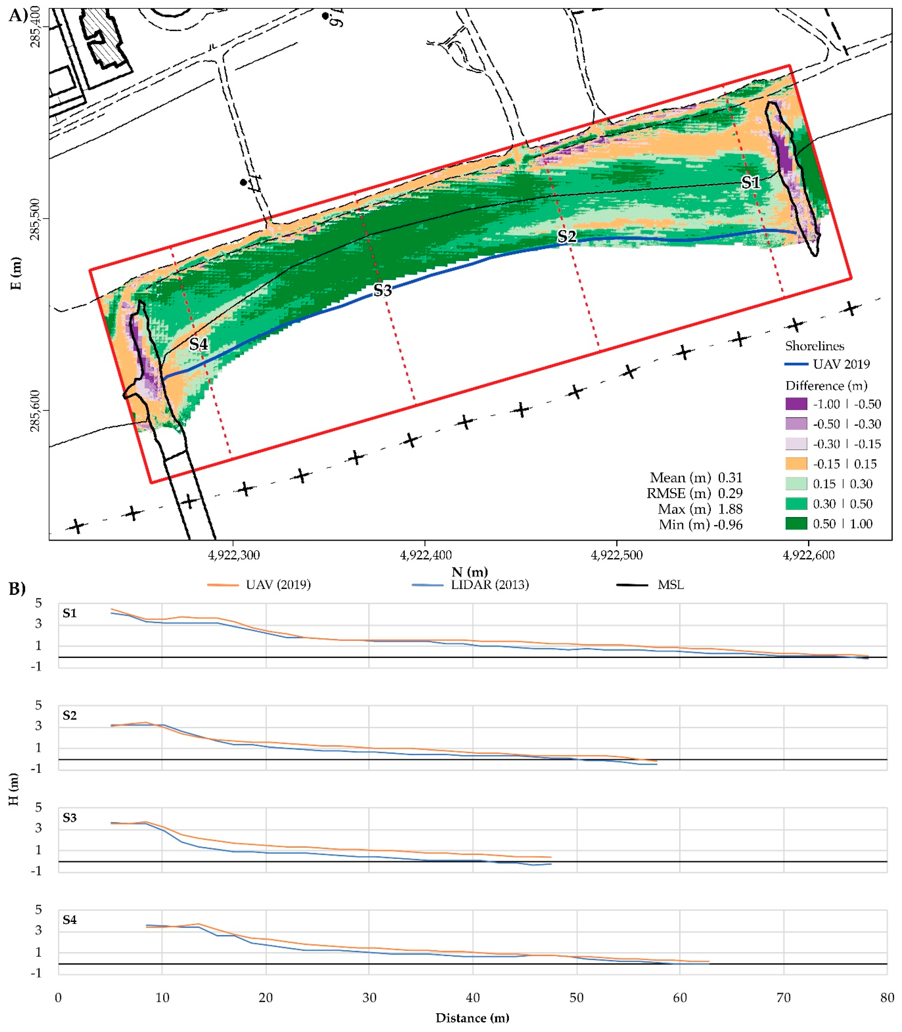
| Data | 07/12/2017 | 25/05/2018 | 24/05/2019 |
|---|---|---|---|
| Mean (m) | −0.01 | −0.01 | 0.00 |
| RMSE (m) | 0.09 | 0.10 | 0.02 |
| Max (m) | 0.24 | 0.83 | 0.06 |
| Min (m) | 0.06 | 0.03 | 0.01 |
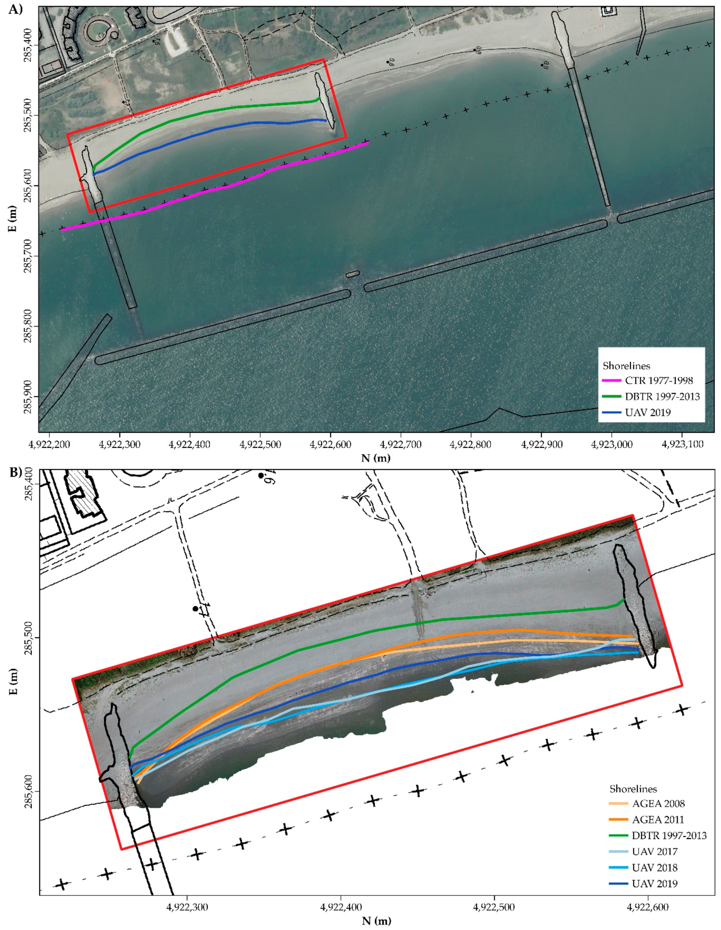
| Source | CTR | DBTR | AGEA | AGEA |
|---|---|---|---|---|
| Date | 1977–1998 | 1977–2013 | 2008 | 2011 |
| S1 | −53.77 | 26.56 | 3.36 | 7.98 |
| S2 | −76.29 | 25.69 | 7.81 | 14.32 |
| S3 | −81.11 | 29.83 | 13.51 | 13.56 |
| S4 | −71.23 | 15.98 | −0.30 | 0.49 |
| Mean (m) | −70.60 | 24.52 | 6.10 | 9.09 |
| Std Dev (m) | 11.92 | 5.96 | 5.95 | 6.39 |
| Max (m) | −53.77 | 29.83 | 13.51 | 14.32 |
| Min (m) | −81.11 | 15.98 | −0.30 | 0.49 |
© 2020 by the authors. Licensee MDPI, Basel, Switzerland. This article is an open access article distributed under the terms and conditions of the Creative Commons Attribution (CC BY) license (http://creativecommons.org/licenses/by/4.0/).
Share and Cite
Zanutta, A.; Lambertini, A.; Vittuari, L. UAV Photogrammetry and Ground Surveys as a Mapping Tool for Quickly Monitoring Shoreline and Beach Changes. J. Mar. Sci. Eng. 2020, 8, 52. https://doi.org/10.3390/jmse8010052
Zanutta A, Lambertini A, Vittuari L. UAV Photogrammetry and Ground Surveys as a Mapping Tool for Quickly Monitoring Shoreline and Beach Changes. Journal of Marine Science and Engineering. 2020; 8(1):52. https://doi.org/10.3390/jmse8010052
Chicago/Turabian StyleZanutta, Antonio, Alessandro Lambertini, and Luca Vittuari. 2020. "UAV Photogrammetry and Ground Surveys as a Mapping Tool for Quickly Monitoring Shoreline and Beach Changes" Journal of Marine Science and Engineering 8, no. 1: 52. https://doi.org/10.3390/jmse8010052
APA StyleZanutta, A., Lambertini, A., & Vittuari, L. (2020). UAV Photogrammetry and Ground Surveys as a Mapping Tool for Quickly Monitoring Shoreline and Beach Changes. Journal of Marine Science and Engineering, 8(1), 52. https://doi.org/10.3390/jmse8010052