Article

Shoreline Extraction Based on an Active Connection Matrix (ACM) Image Enhancement Strategy

by
Sara Zollini
1,*,†,
Maria Alicandro
1,†,
María Cuevas-González
2,†,
Valerio Baiocchi
3,†,
Donatella Dominici
1,† and
Paolo Massimo Buscema
4,5,†
1
DICEAA, Department of Civil, Environmental Engineering and Architecture, Via Gronchi 18, 67100 L’Aquila, Italy
2
Centre Tecnològic de Telecomunicacions de Catalunya (CTTC), Division of Geomatics, Av. Gauss 7, E-08860 Castelldefels, Barcelona, Spain
3
DICEA, Sapienza University of Rome, via Eudossiana, 18, 00184 Roma, Italy
4
Semeion Research Center of Sciences of Communication, Via Sersale 117, 00128 Rome, Italy
5
Department of Mathematical and Statistical Sciences, University of Colorado, Denver, CO 82017, USA
*
Author to whom correspondence should be addressed.
These authors contributed equally to this work.
J. Mar. Sci. Eng. 2020, 8(1), 9; https://doi.org/10.3390/jmse8010009
Submission received: 19 November 2019 / Revised: 6 December 2019 / Accepted: 17 December 2019 / Published: 23 December 2019
(This article belongs to the Special Issue Remote Sensing in Coastline Detection)

Abstract

:
Coastal environments are facing constant changes over time due to their dynamic nature and geological, geomorphological, hydrodynamic, biological, climatic and anthropogenic factors. For these reasons, the monitoring of these areas is crucial for the safeguarding of the cultural heritage and the populations living there. The focus of this paper is shoreline extraction by means of an experimental algorithm, called J-Net Dynamic (Semeion Research Center of Sciences of Communication, Rome, Italy). It was tested on two types of image: a very high resolution (VHR) multispectral image (WorldView-2) and a high resolution (HR) radar synthetic aperture radar (SAR) image (Sentinel-1). The extracted shorelines were compared with those manually digitized for both images independently. The results obtained with the J-Net Dynamic algorithm were also compared with common algorithms, widely used in the literature, including the WorldView water index and the Canny edge detector. The results show that the experimental algorithm is more effective than the others, as it improves shoreline extraction accuracy both in the optical and SAR images.

1. Introduction

The coastal environment is an extraordinary natural resource, not only from the point of view of the cultural heritage but for hosting resources that can be measured in terms of economic assets. It is a dynamic environment, subject to continuous and constant transformation. The coastal area is indeed a highly dynamic system where erosion and deposition phenomena are influenced by various factors. According to [1], the factors responsible for changes in coastal areas may be grouped into geological and geomorphological, hydrodynamic, biological, climatic and anthropogenic factors. The coastal environment, where large percentages of the global population live, change rapidly due to its dynamic nature. For this reason, the availability of up-to-date information on its state is of great interest.
The theoretical definition of “shoreline” is merely the transition between the sea and the land [2,3], and in general, between the land surface and the surface of a water body, such as an ocean, sea or lake. The coastal zone is, instead, that area of land and water that borders the shoreline and extends landward [4]. In [5,6,7] other definitions about coastal areas can be found. In theory, the concept is very simple and intuitive but its application is actually a complex task because of the temporal variability of the shoreline itself. The temporal variability develops on scales profoundly different from instantaneous to secular variations, and it depends on various factors, including wave motion, tides and winds, but also erosion and deposition. For this reason, the results obtained from surveys on the field or remote sensing are generally indicators of the actual shoreline.
According to [7], there are three main subdivisions of shoreline indicators:
  • Characteristics visible by an operator on an aerial or remote sensing image;
  • Intersection between a tidal datum and a digital terrain model or a coastal profile;
  • Characteristics of multispectral images identified by automatic algorithms not necessarily visible to an unaided operator.
In this work, we will experiment with several indicators of the third type by comparing them with each other and with those of the first type. It is important to underline, however, that those things which are extracted are indicators of the shoreline and not the shoreline itself.
Several survey methodologies are used for the detection of shorelines: from traditional topographical and GNSS (Global Navigation Satellite System) surveys to remote sensing techniques (aerial and unmanned aerial vehicle (UAV) photogrammetry, video systems and satellite optical and SAR images [8,9]), as widely discussed in another recent work [10]. In the last few years, the use of optical and SAR satellite images for automatic and semi-automatic shoreline extraction has complemented the traditional approach based on surveying methods and air-photo processing [11]. Several approaches have been proposed to outline the shoreline using remote sensing, such as edge detection, segmentation and classification approaches [6].
An edge in an image is a boundary where there is a change in some physical parameters and it is like a contour between two different regions. Many approaches have been used for edge extraction; for example, the Canny edge detector [12,13] or the snake model [14]. Segmentation methods can be divided into three categories: threshold-based, region-based and edge-based [15]. Concerning classification, they can be pixel-oriented, based on individual pixel classifications or object-oriented—which instead are able to group characteristics by aggregation in similar regions or polygons. Among the pixel-oriented classification, spectral indices have been successfully used to extract shorelines. In particular, water indices (WIs) and vegetation indices (VIs) have been developed, which are obtained by combining two or more spectral bands. Although VIs are mainly used for vegetation analysis, they have also been tested for shoreline mapping purposes [10,16]. WIs have been specifically developed for water body detection [17].
In this work, an experimental algorithm, called J-Net Dynamic [18,19], was tested both on a very high resolution (VHR) WorldView-2 optical image, and for the first time, on a high resolution (HR) Sentinel-1 SAR image. The J-Net Dynamic algorithm can be considered an edge operator, as it highlights the edges of the image and is part of the active connection matrix (ACM) system, which is a new unsupervised artificial adaptive system developed by Semeion Research Institute. The system can automatically extract features of the images—edges, tissue differentiation, etc., when they are activated by original non-linear equations. ACM activation reduces the image noise while maintaining the spatial resolution of high contrast structures. The J-Net Dynamic exploits the dynamic connections between a central pixel and its neighboring pixels. The relationships among these latter pixels with their neighbors is also taken into account, so the new image is created considering the totality of these contributions at every elaboration cycle. Every single neighbor pixel participates in the evolution of the ACM, which is finally used to create the pixel matrix with the new image. A detailed description of the algorithm can be found in Appendix A.

2. Study Area and Data Set

The Abruzzo region (Italy) coastline has a length of 125 km, of which 26 km is high coast and 99 km is sandy coast; the latter, therefore, accounts for 80% of the entire coastline and more than 50% is under erosion. The northern sector, between the Tronto River and Ortona, is characterized by low coasts; proceeding southwards, the coast is formed, up to Vasto, by mainly high coasts, but, at Vasto Marina and San Salvo the coasts are low and sandy. The average width of the Abruzzo beaches is often less than 100 m, and in some cases, it does not reach 50 m. The dominant winds are the Mistral and the Tramontana. Studies performed on wave measurements demonstrated that among the states of significant sea, that is wave heights greater than 0.5 m, the most frequent waves have heights greater than two meters and the most intense wave motions have heights between 3.5 and 6 m, characterized by an occurrence frequency of less than 5% [20].
The study of this paper was conducted on the sandy coast of Ortona (Abruzzo Region) in which three erosion phenomena have been reported on the coast, four active landslides that have effects on the coast and three landslide crags on the sea [21]. For this reason, according to the guidelines for the defense of the coast against erosion and the effects of climate change [22], one of the fundamental elements of a coastal information system is the extraction of the shoreline. The potential of the J-Net Dynamic algorithm for identifying the shoreline, in automatic or semiautomatic mode, from remote sensing, has been tested on two types of images: multispectral WorldView-2 and SAR Sentinel-1 satellite images. The Digital Globe WorldView-2 sensor, launched in October 2009, was the first VHR, 8-band, multispectral commercial satellite [23] with four standard (red, green, blue and near-infrared) and four new (coastal, yellow, red edge and near-infrared) spectral bands [24]. The images are provided with a panchromatic band (0.5 m) and eight multispectral bands (2 m) [25]. Moreover, depending on the level of processing, the images can be supplied as “Basic,” “Standard,” “Ortho Ready Standard Imagery” or “Stereo Pair” products [26]. A WorldView-2 image acquired on 29 June 2010 was analyzed in this work. This image was projected to UTM WGS84 reference system (WGS84/UTM Zone 33 N, EPSG: 32633). After pre-processing, described in Section 3.1, a pan-sharpening pre-treatment was also performed to merge the high geometric resolution of the panchromatic image with the multispectral bands. A Sentinel-1 SAR image has also been analyzed in this work. The Sentinel-1 mission is the European Radar Observatory for the Copernicus joint initiative of the European Commission (EC) and the European Space Agency (ESA) [27]. Sentinel-1 images are freely available and are also supplied with a level of processing that guarantees immediate use: level-0 provides raw images, level-1 Single Look Complex (SLC), level-1 Ground Range Detected (GRD), level-2 Ocean. Seven Sentinel-1 Interferometric Wide (IW) Level-1 (GRD) images (see Table 1) have been downloaded from Copernicus Open Access Hub website [28].
They consist of focused SAR data that have been detected, multi-looked and projected to ground range using the Earth ellipsoid model WGS84. The ellipsoid projection of the GRD products is corrected using the terrain height specified in the product general annotation. The terrain height varies in azimuth but is constant in range (but can be different for each IW sub-swath) [29]. The IW swath acquires data with 250 km swath at 5 m by 20 m spatial resolution. IW captures three sub-swaths using Terrain Observation with Progressive Scans SAR (TOPSAR) [30]. Ground range coordinates are the slant range coordinates projected onto the ellipsoid of the Earth. Pixel values represent detected amplitude. There is no information about the phase. The resulting product has approximately square resolution pixels and square pixel spacing with reduced speckle but reduced spatial resolution. For the IW GRD products, multi-looking is performed on each burst individually. All bursts in all sub-swaths are then seamlessly merged to form a single, contiguous, ground range detected image per polarization. Seven Sentinel-1 images are processed in order to better remove the speckle, although just the one in the middle was processed for shoreline extraction.
Information regarding tides was also taken into account to compare the instantaneous shoreline [31]. In Ortona area, the maximum high tide recorded in the tide tables is 0.6 m and the minimum height is –0.2 m, referenced to mean lower low water (MLLW). As the wave action on the Mediterranean coast is limited [32] the images can be considered at the same tidal moment.

3. Methodology

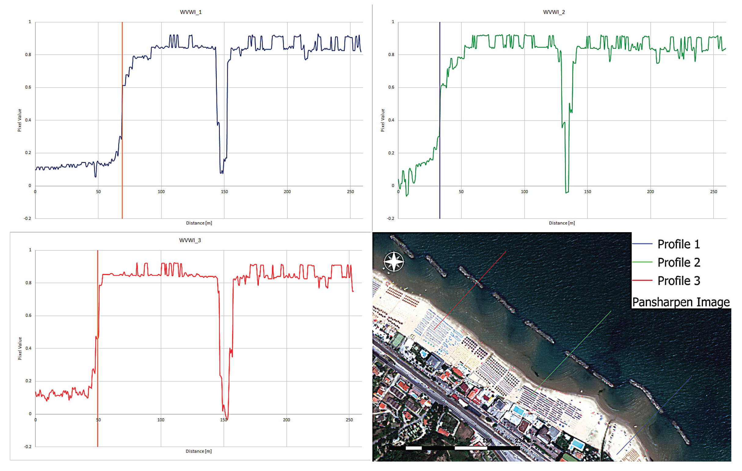
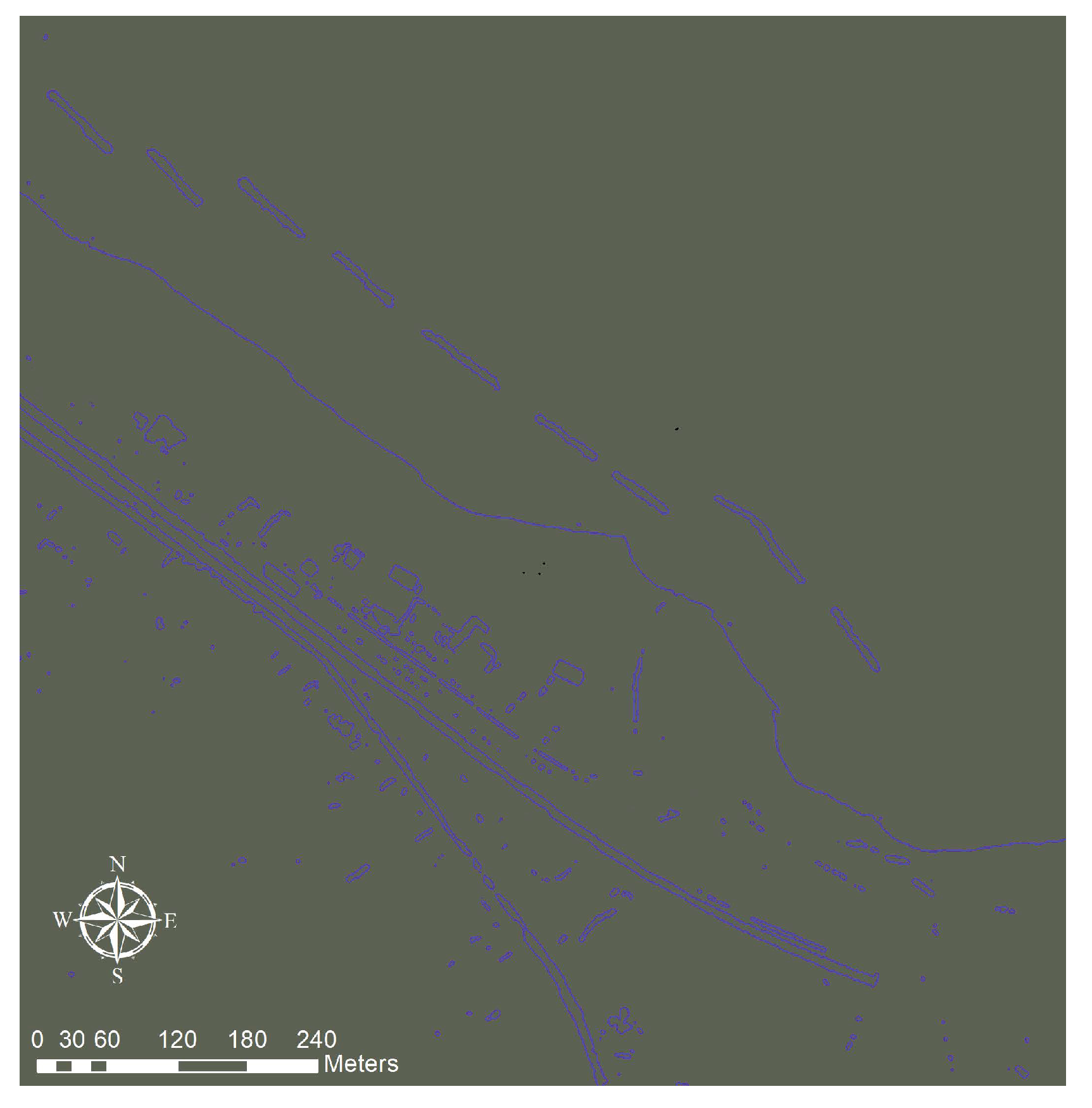
3.1. Shoreline Extraction with WorldView-2 Image

The WorldView-2 images are provided as Ortho Ready Standard products, so a pre-processing is required to correct the geometric distortions [16]. An orthorectification was performed using ERDAS Imagine 2015 [33], and rational polynomial coefficients (RPCs) were used to correct the geometric distortions. In addition, 17 ground control points (GCPs) and 8 check points (CPs) were used to improve the process [10]. Finally, the original spatial resolution of the multi-spectral bands was improved with the panchromatic one by applying the HCS (hyperspherical color dpace) resolution merge algorithm, designed for WorldView-2 [34] and implemented in Erdas Imagine. After the pre-processing, two algorithms were applied to extract the shoreline edges: the WVWI (WorldView Water Index) and the J-Net Dynamic. The WVWI (1) is a WI adjusted for the WorldView-2 images [35] and defined as:
W V W I = C B N I R 2 C B + N I R 2 ,
where C B and N I R 2 are referred to the Coastal band (400–450 nm) and Near Infrared 2 band (860–900 nm), respectively. WVWI combines the Coastal and the Near-Infrared 2 bands pixel by pixel and it ranges mathematically between 1 and 1. WVWI tends to 1 in the presence of water and to 0 where sand is present. To vectorize the shoreline extracted from WVWI, a threshold was set in correspondence of the inflection point evaluated on some WVWI profiles, as it was determined in [36] and in a previous work [10] (Figure 1). The peaks, showed around 150 m on the profile, correspond to the rocks but, for the purpose of this paper, they were not taken into account.
A reclassification based on the threshold was performed and finally the shoreline was digitized with the Arcscan tools in ArcMap (ESRI, Redlands, California). Finally, a smoothing algorithm was used to improve the quality of vector line [37].
The J-Net Dynamic algorithm has been tested on a single band or band combinations. For the sake of brevity, in this work only the analysis of the NIR2 band, which gave the best results, is reported. The NIR2 band is indeed suitable for discriminating water from wet and dry sand, as it is almost completely absorbed by the water and possible perturbations are minimized by the shallow bottoms [38,39].
The J-Net Dynamic algorithm, thoroughly described in the Appendix A, permits one to obtain a clear separation threshold between water and land (Figure 2).
The vectorization of the shoreline extracted by J-Net is performed in the same way of the WVWI.

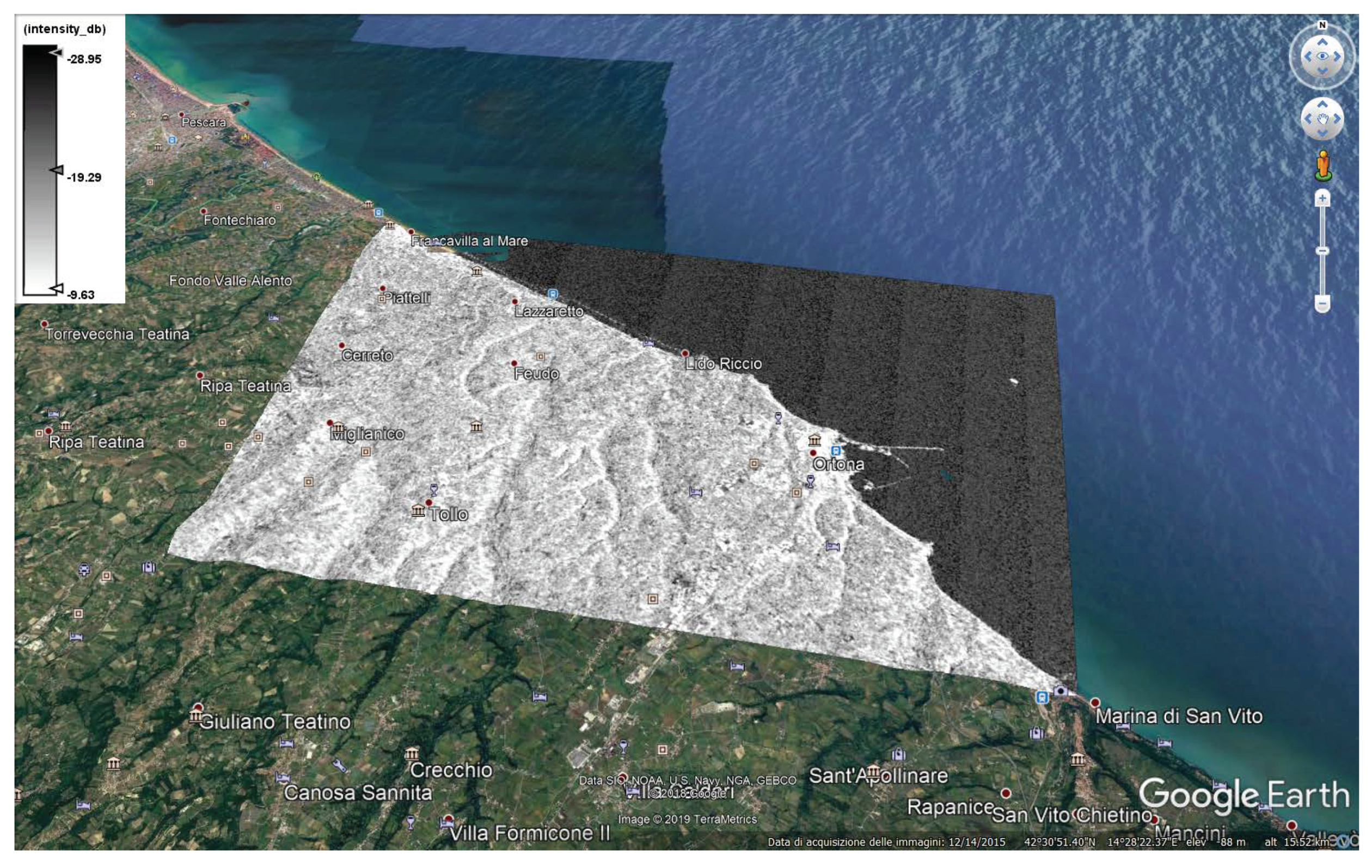
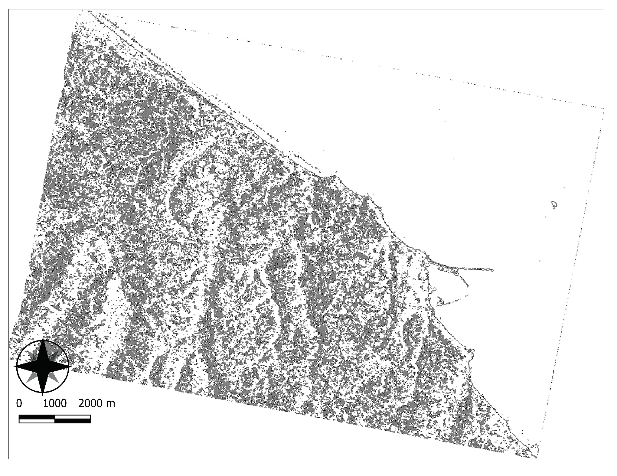
3.2. Shoreline Extraction with Sentinel-1 Image

The pre-processing of Sentinel-1 images is a key issue of SAR elaboration because, for a better identification of the shoreline, it is essential to improve the image quality, and in this case, to reduce noise while preserving the edges. Pre-processing methods can be grouped into noise reduction and image correction [6]. SAR images are affected by speckle, an effect caused by the coherent radiation used by radar systems. It is like a salt and pepper effect that happens because each resolution cell associated with an extended target contains several scattering centers whose elementary returns, by positive or negative interference, originate light or dark image brightness [40]. There are some adaptive filters, such as the median filter, which are suitable for SAR speckle removal. The median filter uses the median values within a moving kernel in place of each pixel of the image. That way, it smooths the image without smoothing the edges [6]. The SNAP (Sentinel Application Platform) software is used to pre-process the Sentinel-1 SAR images. The pre-processing steps that were carried out are:
  • Thermal noise removal;
  • Apply Orbit filer;
  • Calibration to Beta0;
  • Coregistration;
  • Multitemporal de-speckle;
  • Range doppler terrain correction.
The pre-processing aims to enhance the image for a better interpretation. In particular, the purpose is to increase the contrast while preserving the edges, using bands, algorithms and polarizations which maximize the difference between coast and water. The following options were tested:
  • Use decibel bands or not;
  • Use polarization VV or VH;
  • Choose the filter for the multitemporal de-speckle.
Two masks, one on the sea and one on the mainland, have been created and statistics have been computed using the ENVI software (Harris Geospatial Solutions, Broomfield, Colorado, United States). For each study, the digital number (DN) minimum, maximum, mean and standard deviation are calculated. The results show that the contrast between sea and land is higher using the decibel bands and VH polarization. Among the filters computed with SNAP to reduce the speckle, the one which maximizes the contrast is the IDAN, but it presents the problem of excessively smoothing the edges. For this reason, the Lee filter is used, because it is a good compromise between keeping the spatial resolution and preserving the edges [41,42,43].
Finally, the image selected for analysis and shoreline extraction was the one in decibels, with the VH polarization and whose speckle had been reduced using the Lee filter. Figure 3 shows the image acquired on December 31, 2016 after the pre-processing.
After image pre-processing, edge detection algorithms are used to extract the shoreline. It is also manually vectorized to create a reference. As reference shoreline, both an orthorectified Sentinel-2, acquired on 1 January 2017, and the Sentinel-1 on 31 December 2016 itself were used. Due to the inherent characteristics of the SAR images, a better reference line can derive from orthoimagery. This is the reason why the Sentinel-2 optical image was also used as reference. As it was given already orthorectified, it was pre-processed by applying the atmosphere correction using the Sen2Cor tool in SNAP, and then, it was resampled to 10 m. Finally, for the same reason previously explained in Section 3.1, the NIR band (that is band 8 in Sentinel-2) was chosen to extract the reference shoreline. Then, two edge detection algorithms were tested. The first one is the Canny edge detector, which detects a wide range of edges in raster images and produces thin edges as a raster map. It operates, at first, with a Gaussian filter (based on normal distribution) to reduce the noise, then two orthogonal gradient images are computed. Finally, only relevant or significant edges are extracted by thresholding with hysteresis [44]. The result is shown in Figure 4.
Then, the J-Net Dynamic algorithm was tested. The result provided by the J-Net Dynamic algorithm on the SAR image is shown in Figure 5.

4. Results and Discussion

The shorelines extracted from the WorldView-2 image are presented in Figure 6: the red line illustrates the shoreline extracted manually, while the yellow one is the one generated using the WVWI and the blue one from the J-Net Dynamic.
The three instantaneous shorelines extracted using the Sentinel-1 image are shown in Figure 7: the red one is the shoreline extracted manually, the yellow one is from the Canny algorithm and the blue one is from the J-Net Dynamic algorithm. The additional green line is the shoreline manually extracted from Sentinel-2, acquired on 1 January 2017; that is, one day after the Sentinel-1. It was also used as a reference for the reasons explained in Section 3.2.
In order to compare the accuracy of the obtained shorelines, an index I (2), reported in literature [16,45], is used:
I = S L ,
where S is the area calculated between the shoreline extracted from the algorithm and the shoreline used as reference; and L is the length of the reference line. The index is expressed in meters. The values obtained are shown in Table 2.
The results of the index indicate that the use of J-Net Dynamic algorithm improves the shoreline extraction both in the optical and in the SAR images compared to the common filters. For the optical WorldView-2 image, the index I is equal to 1.67 m using WVWI indexed image and 1.20 m using the J-Net Dynamic derived image. This means that, in the VHR image, the J-Net Dynamic algorithm improves the accuracy by about 28 % . For the SAR Sentinel-1 image, considering as a reference the shoreline extracted from the Sentinel-1 image, the index I is equal to 12.52 m using Canny derived image and 5.86 m with the application of the J-Net Dynamic filter. In brief, in the HR SAR image, the accuracy is increased by about 58 % . Considering as reference the shoreline extracted from Sentinel-2 image, the index I is 66.49 m for the Canny and 60.77 m for the J-Net Dynamic, which means an increase of almost 9 % . All the results proves that the shoreline extracted from the J-Net Dynamic derived image is over-fitted to the reference compared to the ones extracted from the common filters. Two more things can be also noted: the first one is that there is a higher difference between the SAR image values and the optical image values. This happens because the SAR image has a lower resolution. The second one is that, with respect to the SAR image, there is a big difference depending on the chosen reference shoreline. The ones extracted with the algorithms are further away from the Sentinel-2 than the Sentinel-1 reference shoreline. The SAR image, due to its nature, could have little backscattering from the wet sand, which means that, in this case, it “confuses” the wet sand with water. However, the purpose of this paper is to test the J-Net Dynamic on optical and SAR images and to compare the results to the common algorithms. In all of the aforementioned cases, it proved to extract a shoreline closest to the reference one.
To better determine the accuracy of the shoreline extraction, a method already used in literature [10,46] was used. Ten transects (Figure 8), about one every 100 m and drawn from the land to the sea, were used to calculate the intersection between them and the seven shorelines extracted from WorldView-2, WVWI, J-Net Dynamic on the VHR image, Sentinel-1, Sentinel-2, Canny and J-Net Dynamic on the HR image.
Then, the differences between the reference shorelines and the ones extracted from the algorithms were measured. In the end, the mean values and the standard deviations of every difference were calculated (Table 3).
As shown in Table 3, for the VHR image, the standard deviation is 1.13 m and the mean is 1.87 considering the common filter. On the other hand, the standard deviation of the J-Net Dynamic is 1.12 m and the mean value 1.45 m. For the HR image, considering the Sentinel-2 optical image as a reference, the results show that the mean value of the difference with the Canny derived shoreline is 70.11 m and the standard deviation is 29.20 m. Compared with the J-Net values, that are 66.09 m and 19.57 m respectively, they are higher. The same happens considering the Sentinel-1 as a reference: the mean values for Canny and J-Net are 17.21 m and 10.61 m and the standard deviations are 9.10 m and 8.21 m, respectively. It can be noticed that the mean and standard deviation are lower for the VHR optical image than the HR SAR image, as expected. Moreover, the values obtained for the SAR image using two different reference shorelines confirm the better results obtained by using the Sentinel-1 image as references, as they were found previously. Indeed, the standard deviation for the difference between Sentinel-2 and Canny shorelines is 29.20 m, compared to 9.10 m obtained by the difference between the Sentinel-1 and Canny shorelines. The same happens for the differences between the Sentinel-2 with the J-Net (19.57 m) and Sentinel-1 with the J-Net (8.21 m). However, in every case, the J-Net Dynamic gives best accuracy compared to the common filters, as already found out with the index I.
In [16], the index I was used to compare the results obtained for the shoreline extraction using the NDVI and the NDWI (normalized difference water index, which considers the same bands of WVWI and the same equation) filters on the WorldView-2 initial and pansharpened image. It confirms that NDWI application provides better results; and that the pan-sharpening permits one to enhance geometric resolution and to reduce, to less than 1 m, the mean value of shifts between the automatically extracted shoreline and the manually vectorized one. They found an index value of 1.386 m for the multispectral image and 0.955 m for the pan-sharpened one. The better accuracy, compared to the one obtained for the research of this paper, that is, 1.67 m, could be due to the fact that they identified a different threshold to detect the shoreline based on a classification method using three contrasting classes (sea, land and vegetation) or due to the fact that the range of shoreline was both sandy and rocky. The rocky parts are less sensitive to instantaneous dynamic change than the sandy ones. The index I was also considered to evaluate the average shift between two temporal consecutive shorelines [11]. They compared shorelines during 2005 and 2011 and they evidenced that the effects of the human intervention, like the installation of breakwaters, limit erosion phenomena near shore zone. This tendency was also remarked on for the years 2011–2012.
The index I has not been used yet in literature to assess the SAR images. In [47], an automated method of the shoreline position detection using Sentinel-1 SAR image was studied. The method aimed at the automatic extraction of shoreline edge from pre-processed images. The algorithm performs four steps: despeckling, binarisation, morphological operations and edge detection by means of the Canny edge detector. Once the shoreline is extracted, it is compared to the one extracted from the images acquired by video system. The VDS (video-derived shoreline) is a collection of shoreline points. So, the distance between each point from the SDS (satellite-derived shoreline) is calculated in order to evaluate quantitatively the correctness of the SDS position. The average offset turns out to be about 10 m and the root mean square difference (RMSD) is 12.48 m.
To compare the accuracy with the case study discussed in this paper, the vertices of the reference shoreline (so the shoreline manually outlined on the pre-processed Sentinel-1 image) are extracted and the shortest distance between them and the Canny derived shoreline is calculated. The results show that the average offset is around 16 m, while the standard deviation is 11.40 m. So, a robust contrast can be performed also by applying the binarisation, as proposed by [47], because it splits exactly water and land, and as consequence, the edge detector can easily extract the contour of the image. To increase the accuracy, [48] propose an integration between RASAT pansharpened image and Sentinel-1 SAR image to improve the quality of the results. The first land/water segmentation was obtained using RASAT image by means of random forest classification method. Then, the result was used as training data set to define fuzzy parameters for shoreline extraction from Sentinel-1A SAR image. The manually digitized shoreline was used as a reference and the accuracy assessment was performed by calculating perpendicular distances between reference data and extracted shoreline by the aforementioned method. The mean distance value between the final result and the reference data was calculated to be 5.59 m, which is half pixel size of Sentinel-1A and which is almost three times better then the results obtained in this research. The higher accuracy was due not only to the integration between optical and SAR images, but also to the fact that the coast considered in [48] is mainly stony rather than sandy.
Due to the high resolution difference, the authors find it inappropriate to compare the WorldView-2 optical image and the Sentinel-1 SAR image. The purpose of the paper was only to discuss potentiality of the J-Net Dynamic algorithm both in optical and in SAR images independently. So, an additional test was performed. To compare the accuracy with the average offset obtained by means of the Canny edge detector (16 m with an RMSD equal to 11.40), the vertices of the pre-processed Sentinel-1 image shoreline were extracted and the shortest distance between them and the J-Net derived shoreline was calculated. An average offset around 7 m and a standard deviation of 7.36 m were found. The accuracy was lower than one pixel. The values confirm the trend that was delineated by means of the index I value: the algorithm J-Net Dynamic increased the accuracy of the extraction.
In future studies, other images, comparable in terms of resolution, such as Sentinel-1 and Sentinel-2 or WorldView-2 and COSMO-SkyMed images, can be integrated to improve the accuracy of the results. Moreover, to answer to the question of whether the Sentinel-1 is capable of monitoring coastal changes, another interesting future work could consider all the Sentinel-1 image data set to study the shoreline changes during a determined period of time.

5. Conclusions

Monitoring coastal areas with shoreline mapping allows one to analyze erosion and deposition phenomena in order to be able to propose corrective actions. In this work, an experimental algorithm, called J-Net Dynamic, has been presented to automatically extract the shoreline. It has been tested both in multispectral and in SAR images with different resolutions. Both images were pre-processed to improve their geometric and radiometric properties in order to facilitate their subsequent analysis. They were then processed with filters and indices commonly used for this kind of research, like the WorldView water index for the optical image and the Canny edge detector for the radar image, and the J-Net Dynamic. The J-Net Dynamic algorithm was mainly developed and previously applied in medical fields and it has been tested on a VHR optical image, and for the first time, also on an HR SAR image for environmental monitoring. To validate and verify the accuracy and robustness of this approach, a comparison with other typical algorithms was performed through an index I, which divides the area between the shoreline obtained by the algorithm and the reference one with the length of the latter, and through the use of ten transects along the shorelines. The results showed that J-Net Dynamic improves the detection, obtaining a shoreline closest to the reference, both for VHR and HR satellite images.

Author Contributions

These authors contributed equally to this work. All authors have read and agreed to the published version of the manuscript.

Funding

This research received no external funding.

Conflicts of Interest

The authors declare no conflict of interest.

Abbreviations

The following abbreviations are used in this manuscript:
VHRvery high resolution
HRhigh resolution
SARsynthetic aperture radar
GNSSGlobal Navigation Satellite System
UAVunmanned aerial vehicle
WIwater index
VIvegetation index
ACMactive connections matrix
UTMuniversal transverse mercator
WGS84World Geodetic System 1984
EPSGEuropean Petroleum Survey Group
ECEuropean Commission
ESAEuropean Space Agency
SLCsingle look complex
GRDground range detected
IWInterferometric Wide
TOPSARTerrain Observation with Progressive Scans SAR
MLLWmean Lower low water
RPCrational polynomial coefficient
GCPground control point
CPcheck point
HCShyperspherical color space
WVWIWorldView water index
CBcoastal band
NIRnear infrared
SNAPsentinel application platform
DNdigital number
NDVInormalized difference vegetation index
NDWInormalized difference Water Index
VDSvideo-derived shoreline
SDSsatellite-derived shoreline
RMSDroot mean square difference
COSMO-SkyMedCOnstellation of small Satellites for the Mediterranean basin Observation

Appendix A

J-Net Dynamic

This algorithm was developed by Professor Paolo Massimo Buscema, mathematician, Director of the Semeion Research Centre of Science of Communication of Rome and Full Professor Adjoint at the University of Colorado (USA).
The patent concerns active connections matrix systems (ACM), according to which each image is considered as an active matrix (network) of connected elements (pixels) that develops over time. The main idea upon which this theory is based states that each digital image stores the maximum amount of information within the pixel values and their relationships. Furthermore, it is possible to obtain important information by analyzing the reciprocal positions occupied by pixels. For a complete presentation of ACM algorithms, see [18,49].
Any digital image is a matrix made of as many rows as the pixels that determine the width and as many columns as the pixel number related to the height. Each pixel is identified by its coordinates i 1 , , R , j 1 , , C , and its brightness L 2 M (e.g., in the case of 256 shades of gray, M = 8). For each pixel u i j a set containing all the surrounding pixels I ( u i j ) named neighborhood can be defined. In the ACM systems, all the pixels u x y I ( u i j ) are linked to the central pixel u i j by means of the w ( i j ) , ( x y ) connections. The systems are classified into three orders of complexity, according to the type of evolution over time. In the first order of complexity, the values of connections are initialized once, at the beginning, and then remain fixed while pixel values u i j [ n ] evolve over time until convergence, starting from the u i j [ 0 ] value, directly derived from the image. The situation is specular in the case of second order, where the pixels’ values are fixed and equal to u i j [ 0 ] , while the connections values w ( i j ) , ( x y ) [ n ] are updated at each iteration, after initializing them to values w ( i j ) , ( x y ) [ 0 ] 0 . Finally, the third order of complexity includes models in which both the pixels and the connections change over time.
J–Net Dynamic [19,49] is a ACM system with dynamic connections and units (third order of complexity). The main prerogative of this method is to consider in its equations not only the central pixel as such, with its relative neighborhood, but also as part of the surroundings of each of the pixels around it, when they are considered in turn as the central pixel. At the beginning of the process, the units u i j are linearly scaled into the range [ 1 + α , 1 + α ] , where α is a parameter to be set up. By varying the α value it is possible to study images in an iterative manner. The first part of computations involves exclusively the central pixel and its neighborhood I i j , as shown by Equations (A2)–(A7). J–Net follows the schema: update of weights (Equations (A1)– (A5), computation of the new pixel values based on the weights (Equation (A6)), update of units (Equations (A7)–(A14), re-update of weights and so on. In this case, the update of units also involves the neighborhoods I x y such that u x y I i j .
S i j [ n ] = π · ( r i j [ n ] ) 2
D i j [ n ] = ( x y ) s . t . u x y I i j ( u i j [ n ] w ( i j ) , ( x y ) [ n ] )
J i j [ n ] = e D i j [ n ] e D i j [ n ] e D i j [ n ] + e D i j [ n ]
Δ w ( i j ) , ( x y ) [ n ] = ( u i j [ n ] J i j [ n ] ) · ( 2 · J i j [ n ] ) · ( 1 ( J i j [ n ] ) 2 ) · ( u x y [ n ] w ( i j ) , ( x y ) [ n ] )
w ( i j ) , ( x y ) [ n + 1 ] = w ( i j ) , ( x y ) [ n ] + Δ w ( i j ) , ( x y ) [ n ]
P i j [ n ] = S P · 1 | I i j | · ( x y ) s . t . u x y I i j w ( i j ) , ( x y ) [ n ] + O P ,
where:
S P = M P M w m w
O P = m w · M P M w m w .
M P denotes the maximum value available for pixels, M w and m w are, respectively, the maximum and the minimum weights w ( i j ) , ( x y ) [ n ] i , x { 1 , , R } and j , y { 1 , , C } .
O u t i j [ n ] = S 0 · 1 | I i j | · ( x y ) s . t . u x y I i j w ( i j ) , ( x y ) [ n ] + O 0
where, with the usual notation:
S 0 = 2 M w m w
O 0 = M w + m w M w m w .
The internal activation state of each pixel is then defined as:
S i j [ n ] = | O u t i j [ n ] | .
Therefore, the closer the weighted average of the connections of each pixel with those of its surroundings is to a neutral value, 0 or 127 depending on the encoding, the higher the value of the internal activation state of the pixel itself. With the aim of defining an update rule for units, the quantity Δ S ( i j ) , ( x y ) [ n ] is considered (Equation (A9). Then, according to Equations (A10)–(A11), the transition from I i j to I x y takes place.
Δ S ( i j ) , ( x y ) [ n ] = t a n h ( S i j [ n ] u x y [ n ] )
φ i j [ n ] = L · u i j [ n ] · ( x y ) s . t . u x y I i j 1 Δ S ( x y ) , ( i j ) [ n ] 2
ψ i j [ n ] = ( x y ) s . t . u x y I i j t a n h ( φ x y [ n ] ) .
The delta quantities required for correction shall be calculated in the last step. It is possible to choose for two different update laws named union (Equation (A12)) and intersection (Equation (A13)).
δ u i j [ n ] = φ i j [ n ] + ψ i j [ n ]
δ u i j [ n ] = φ i j [ n ] · ψ i j [ n ]
u i j [ n + 1 ] = u i j [ n ] + δ u i j [ n ] .

References and Note

  1. Łabuz, T.A. Environmental impacts-coastal erosion and coastline changes. In Second Assessment of Climate Change for the Baltic Sea Basin; Springer: Cham, Switzerland, 2015; pp. 381–396. [Google Scholar]
  2. Carapuço, M.M.; Taborda, R.; Silveira, T.M.; Psuty, N.P.; Andrade, C.; Freitas, M.C. Coastal geoindicators: Towards the establishment of a common framework for sandy coastal environments. Earth-Sci. Rev. 2016, 154, 183–190. [Google Scholar] [CrossRef]
  3. Dolan, R.; Hayden, B.P.; May, P.; May, S. The reliability of shoreline change measurements from aerial photographs. Shore Beach 1980, 48, 22–29. [Google Scholar]
  4. Sorensen, R.M. Basic Coastal Engineering; Springer Science & Business Media: New York, NY, USA, 2005; Volume 10. [Google Scholar]
  5. Gens, R. Remote sensing of coastlines: Detection, extraction and monitoring. Int. J. Remote Sens. 2010, 31, 1819–1836. [Google Scholar] [CrossRef]
  6. Toure, S.; Diop, O.; Kpalma, K.; Maiga, A.S. Shoreline Detection using Optical Remote Sensing: A Review. ISPRS Int. J. Geo-Inf. 2019, 8, 75. [Google Scholar] [CrossRef] [Green Version]
  7. Boak, E.H.; Turner, I.L. Shoreline definition and detection: A review. J. Coastal Res. 2005, 688–703. [Google Scholar] [CrossRef] [Green Version]
  8. Pugliano, G.; Robustelli, U.; Luccio, D.D.; Mucerino, L.; Benassai, G.; Montella, R. Statistical Deviations in Shoreline Detection Obtained with Direct and Remote Observations. J. Mar. Sci. Eng. 2019, 7, 137. [Google Scholar] [CrossRef] [Green Version]
  9. Palazzo, F.; Latini, D.; Baiocchi, V.; Del Frate, F.; Giannone, F.; Dominici, D.; Remondiere, S. An application of COSMO-Sky Med to coastal erosion studies. Eur. J. Remote Sens. 2012, 45, 361–370. [Google Scholar] [CrossRef] [Green Version]
  10. Dominici, D.; Zollini, S.; Alicandro, M.; Della Torre, F.; Buscema, P.M.; Baiocchi, V. High Resolution Satellite Images for Instantaneous Shoreline Extraction Using New Enhancement Algorithms. Geosciences 2019, 9, 123. [Google Scholar] [CrossRef] [Green Version]
  11. Maglione, P.; Parente, C.; Vallario, A. High resolution satellite images to reconstruct recent evolution of domitian coastline. Am. J. Appl. Sci. 2015, 12, 506. [Google Scholar] [CrossRef] [Green Version]
  12. Liu, H.; Jezek, K.C. Automated extraction of coastline from satellite imagery by integrating Canny edge detection and locally adaptive thresholding methods. Int. J. Remote Sens. 2004, 25, 937–958. [Google Scholar] [CrossRef]
  13. Zhang, T.; Yang, X.; Hu, S.; Su, F. Extraction of coastline in aquaculture coast from multispectral remote sensing images: Object-based region growing integrating edge detection. Remote Sens. 2013, 5, 4470–4487. [Google Scholar] [CrossRef] [Green Version]
  14. Sheng, G.; Yang, W.; Deng, X.; He, C.; Cao, Y.; Sun, H. Coastline detection in synthetic aperture radar (SAR) images by integrating watershed transformation and controllable gradient vector flow (GVF) snake model. IEEE J. Ocean. Eng. 2012, 37, 375–383. [Google Scholar] [CrossRef]
  15. Ma, H.; Zhang, L. Ocean SAR Image Segmentation and Edge Gradient Feature Extraction. J. Coast. Res. 2019, 94 (Suppl. S1), 141–144. [Google Scholar] [CrossRef]
  16. Maglione, P.; Parente, C.; Vallario, A. Coastline extraction using high resolution WorldView-2 satellite imagery. Eur. J. Remote Sens. 2014, 47, 685–699. [Google Scholar] [CrossRef]
  17. McFeeters, S.K. The use of the Normalized Difference Water Index (NDWI) in the delineation of open water features. Int. J. Remote Sens. 1996, 17, 1425–1432. [Google Scholar] [CrossRef]
  18. Buscema, P.M. Sistemi ACM e Imaging Diagnostico: Le Immagini Mediche Come Matrici Attive di Connessioni; Springer Science & Business Media: New York, NY, USA, 2006. [Google Scholar]
  19. Buscema, M.; Catzola, L.; Grossi, E. Images as active connection matrixes: The J-net system. Int. J. Intell. Comput. Med. Sci. Image Process. 2008, 2, 27–53. [Google Scholar] [CrossRef]
  20. Le spiagge dell’Abruzzo. Studi costieri. 2006; Volume 10. Available online: http://www.gnrac.it/rivista/Numero10.htm (accessed on 2 December 2019).
  21. Progetto Preliminare Della Costa Teatina—Fenomeni Erosivi Della Fascia Costiera. Available online: http://www.provincia.chieti.it/flex/cm/pages/ServeAttachment.php/L/IT/D/2%252F4%252F4%252FD.d367c153fd7837fd72ca/P/BLOB%3AID%3D3926/E/pdf (accessed on 28 October 2019).
  22. MATTM-Regioni. Linee Guida per la Difesa della Costa dai fenomeni di Erosione e dagli effetti dei Cambiamenti climatici. Versione 2018. Available online: http://www.erosionecostiera.isprambiente.it/linee-guida-nazionali (accessed on 29 October 2019).
  23. European Space Imaging. Available online: https://www.euspaceimaging.com/about/satellites/worldview-2/ (accessed on 19 September 2019).
  24. Satellite Imaging Corporation. Available online: https://www.satimagingcorp.com/satellite-sensors/worldview-2/ (accessed on 19 September 2019).
  25. Geoimage. Available online: https://www.geoimage.com.au/satellite/worldview-2 (accessed on 19 September 2019).
  26. Geomatics. Available online: https://www.https://geomatics.planet.com/upload/digitalglobe/DigitalGlobe%20Core%20Imagery%20Products%20Guide.pdf (accessed on 19 September 2019).
  27. ESA Sentinel Home, Missions, Sentinel-1. Available online: https://sentinel.esa.int/web/sentinel/missions/sentinel-1/overview (accessed on 22 May 2019).
  28. Copernicus Open Access Hub. Available online: https://scihub.copernicus.eu/dhus/#/home (accessed on 22 May 2019).
  29. ESA Sentinel Home, User Guides, Sentinel-1 SAR, Product Types and Processing Levels, Level-1. Available online: https://sentinel.esa.int/web/sentinel/user-guides/sentinel-1-sar/product-types-processing-levels/level-1 (accessed on 22 May 2019).
  30. ESA Sentinel Home, User Guides, Sentinel-1 SAR, Acquisition Modes, Interferometric Wide Swath. Available online: https://sentinel.esa.int/web/sentinel/user-guides/sentinel-1-sar/acquisition-modes/interferometric-wide-swath (accessed on 24 May 2019).
  31. TIDES4FISHING. Available online: https://tides4fishing.com/ (accessed on 29 March 2019).
  32. Whitfield, A.; Elliott, M. 1.07-Ecosystem and biotic classifications of estuaries and coasts. In Treatise on Estuarine and Coastal Science; Elsevier: Amsterdam, The Netherlands, 2011; pp. 99–124. [Google Scholar]
  33. Planetek, ERDAS IMAGINE, Software, PRODUCER Suite of Power Portfolio by Hexagon Geospatial.
  34. Padwick, C.; Deskevich, M.; Pacifici, F.; Smallwood, S. WorldView-2 Pansharpening. In Proceedings of the ASPRS 2010 Annual Conference, San Diego, CA, USA, 26–30 April 2010. [Google Scholar]
  35. Wolf, A.F. Using WorldView-2 Vis-NIR multispectral imagery to support land mapping and feature extraction using normalized difference index ratios. In International Society for Optics and Photonics Algorithms and Technologies for Multispectral, Hyperspectral, and Ultraspectral Imagery XVIII; International Society for Optics and Photonics: San Diego, CA, USA, 2012; Volume 8390. [Google Scholar]
  36. Palomar-Vázquez, J.; Almonacid-Caballer, J.; Pardo-Pascual, J.E.; Sanchez-García, E. SHOREX: A new tool for automatic and massive extraction of shorelines from Landsat and Sentinel 2 imagery. In Proceedings of the 7th International Conference on the Application of Physical Modelling in Coastal and Port Engineering and Science (Coastlab), Santander, Spain, 22–26 May 2018. [Google Scholar]
  37. Bodansky, E.; Gribov, A.; Pilouk, M. Smoothing and compression of lines obtained by raster-to-vector conversion. In International Workshop on Graphics Recognition; Springer: Berlin/Heidelberg, Germany, 2001; pp. 256–265. [Google Scholar]
  38. Alesheikh, A.A.; Ghorbanali, A.; Nouri, N. Coastline change detection using remote sensing. Int. J. Environ. Sci. Technol. 2007, 4, 61–66. [Google Scholar] [CrossRef] [Green Version]
  39. Braga, F.; Tosi, L.; Prati, C.; Alberotanza, L. Shoreline detection: Capability of COSMO-SkyMed and high-resolution multispectral images. Eur. J. Remote Sens. 2013, 46, 837–853. [Google Scholar] [CrossRef]
  40. ESA, Earth Online, Home, Missions, ESA EO Missions, ERS, Instruments, SAR, Applications. Available online: https://earth.esa.int/web/guest/missions/esa-operational-eo-missions/ers/instruments/sar/applications/radar-courses/content-3/-/asset_publisher/mQ9R7ZVkKg5P/content/radar-course-3-image-interpretation-tone (accessed on 3 September 2019).
  41. Marghany, M.; Sabu, Z.; Hashim, M. Mapping coastal geomorphology changes using synthetic aperture radar data. Int. J. Phys. Sci. 2010, 5, 1890–1896. [Google Scholar]
  42. Pradhan, B.; Rizeei, H.; Abdulle, A. Quantitative assessment for detection and monitoring of coastline dynamics with temporal RADARSAT images. Remote Sens. 2018, 10, 1705. [Google Scholar] [CrossRef] [Green Version]
  43. Taha, L.G.E.D.; Elbeih, S.F. Investigation of fusion of SAR and Landsat data for shoreline super resolution mapping: The northeastern Mediterranean Sea coast in Egypt. Appl. Geom. 2010, 2, 177–186. [Google Scholar] [CrossRef] [Green Version]
  44. GRASS Manual. Available online: https://grass.osgeo.org/grass76/manuals/addons/i.edge.html (accessed on 5 July 2019).
  45. Guastaferro, F.; Maglione, P.; Parente, C.; Santamaria, R. Estrazione in automatico della linea di costa da immagini satellitari IKONOS. In Proceedings of the Conference “Geomatica. Le Radici del Futuro. Tributo a Sergio Degual & Riccardo Galetto”, Pavia, Italy, 10–11 February 2011; pp. 109–116, ISBN 88-901939-6-4. [Google Scholar]
  46. Esmail, M.; Mahmod, W.E.; Fath, H. Assessment and prediction of shoreline change using multi-temporal satellite images and statistics: Case study of Damietta coast, Egypt. Appl. Ocean Res. 2019, 82, 274–282. [Google Scholar] [CrossRef]
  47. Spinosa, A.; Ziemba, A.; Saponieri, A.; Navarro-Sanchez, V.D.; Damiani, L.; El Serafy, G. Automatic Extraction of Shoreline from Satellite Images: A new approach. In Proceedings of the 2018 IEEE International Workshop on Metrology for the Sea; Learning to Measure Sea Health Parameters (MetroSea), Bari, Italy, 8–10 October 2018; pp. 33–38. [Google Scholar]
  48. Demir, N.; Oy, S.; Erdem, F.; Şeker, D.Z.; Bayram, B. Integrated shoreline extraction approach with use of Rasat MS and SENTINEL-1A SAR Images. ISPRS Ann. Photogramm. Remote Sens. Spat. Inf. Sci. 2017, 4, 445. [Google Scholar] [CrossRef] [Green Version]
  49. Buscema, M.; Grossi, E. J-Net System: A New Paradigm for Artificial Neural Networks Applied to Diagnostic Imaging. In Applications of Mathematics in Models, Artificial Neural Networks and Arts; Publishing House: Dordrecht, The Netherlands, 2010; pp. 431–455. [Google Scholar]
Figure 1. Spatial profiles of WVWI (WorldView Water Index): along the x-axis the distances (m) and along the y-axis the WVWI pixel values; the vertical line represents the inflection point in which the threshold between water and sand has been set.
Jmse 08 00009 g001
Figure 2. J-Net algorithm tested on NIR2 band of the WorldView-2 image.
Jmse 08 00009 g002
Figure 3. Pre-processed and georeferenced Sentinel-1 image. Date: December 31, 2016. Units: decibels. Polarization: VH polarization. De-speckle filter: Lee.
Jmse 08 00009 g003
Figure 4. Canny algorithms applied on the pre-processed Sentinel-1 image acquired on 31 December 2019.
Jmse 08 00009 g004
Figure 5. Application of the J-Net Dynamic algorithm on the SAR Sentinel-1 image acquired on 31 December 2016.
Jmse 08 00009 g005
Figure 6. WorldView-2 image with three shorelines: the red line is the manually extracted shoreline; the yellow one is generated using the WVWI and the blue one from the J-Net Dynamic algorithm.
Jmse 08 00009 g006
Figure 7. SAR Sentinel-1 image on the background showing four shorelines: the red and the green lines are, respectively, the shorelines manually extracted from Sentinel-1 and Sentinel-2 images; the yellow one is the one generated using the Canny algorithm and the blue one from the J-Net Dynamic algorithm.
Jmse 08 00009 g007
Figure 8. Ten transects every 100 m, drawn from the land to the sea, to calculate the intersection between them and seven shorelines extracted from WorldView-2, WVWI, J-Net Dynamic on the VHR image, Sentinel-1, Sentinel-2, Canny and J-Net Dynamic on the HR image.
Jmse 08 00009 g008
Table 1. List of the Sentinel-1 images used in this analysis.
Sentinel-1 Images
NumberDate dd/mm/yyyy
112/01/2017
206/01/2017
331/12/2016
425/12/2016
519/12/2016
613/12/2016
707/12/2016
Table 2. I Index values. Comparisons.
Image TypeOptical ImageSAR Image
Reference shoreline extracted fromPansharpened WV-2 imageSentinel-1 imageSentinel-2 image
AlgorithmNDVIJ-Net DynamicCannyJ-Net DynamicCannyJ-Net Dynamic
I (m)1.671.2012.525.8666.4960.77
% increase28.1458.198.60
Table 3. Statistic table. The means and the standard deviations have been calculated on the difference between the reference shorelines with the algorithms we tested. The difference has been calculated on the values obtained from the intersection between the transects and the seven shorelines.
VHR OPTICALHR SAR
WV2 - WVWIWV2 - J NetS2 - CannyS2 - J NetS1 - CannyS1 - JNet
Mean (m)1.871.4570.1166.0917.2110.61
Standard deviation (m)1.131.1229.2019.579.108.21

