Hydro-Acoustic and Hydrodynamic Optimization of a Marine Propeller Using Genetic Algorithm, Boundary Element Method, and FW-H Equations

Abstract

Noise generated by ships is one of the most significant noises in seas, and the propeller has a significant impact on the noise of ships, which reducing it can significantly lower the noise of vessels. In this study, a genetic algorithm was used to optimize the hydro-acoustic and hydrodynamic performance of propellers. The main objectives of this optimization were to reduce the propeller noise and increase its hydrodynamic efficiency. Modifying the propeller geometry is one of the most effective methods for optimizing a propeller performance. One of the numerical methods for calculating propeller noise is the Ffowcs Williams and Hawkings (FW-H) Model. A numerical code was developed by authors which solved these equations using the velocity and pressure distribution around the propeller and calculated its noise. To obtain flow quantities and to investigate the hydrodynamic performance of the propeller, a code was developed using a Boundary Element Method, the panel method. The geometry of DTMB 4119 propeller was selected for optimization, where geometric modifications included skew angle, rake angle, pitch to diameter (P/D) distribution, and chord to diameter (c/D) distribution. Finally, the results of geometric optimization were presented as Pareto optimal solutions. The results indicated that the optimum geometries had rake angles between 8.14 and 12.05 degrees and skew angles between 31.52 and 39.74 degrees. It was also observed that the increase in the chord up to a specific limit enhanced the efficiency and reduced the noise of the propeller.

1. Introduction

Marine propellers play an essential role in the maritime industry and shipping. Due to the increasing importance of propellers, extensive research has been carried out on various aspects of design, such as hydrodynamics and hydro-acoustic performance. Nowadays, with the progress in numerical methods and improvements in processors, the geometric optimization of marine propellers can be performed more comprehensively. The purpose of this research is to present an optimization procedure for a marine propeller in terms of generated noise and hydrodynamic efficiency.

The noise generated by the propeller has a significant contribution to the total noise of the ship. In addition to the environmental impacts, the noise of ships can affect the health and comfort of the crew and passengers of the ship [1,2]. For warships, high levels of noise may cause detection and possible dangers for the ship. Furthermore, the hydrodynamic optimization of the propeller and elevation of the propulsion efficiency could reduce the ship’s fuel consumption and relevant costs. In some cases, reducing the noise of a propeller may lead to the reduction of propeller efficiency, which may be admissible for propellers of warships.

In previous research on marine propellers, in most cases, only one aspect of the design, hydrodynamic performance or generated noise has been studied, and multi-objective optimization has not been carried out. Meanwhile, the number of geometries investigated has been limited. In this study, thanks to the higher solution speed compared to previous methods, a large number of geometries will be studied.

In geometric optimization of the propeller using the genetic algorithm method, hydrodynamic analysis for each geometry must be performed. Then, using the output of the previous step, the noise of propeller is calculated. Through computational fluid dynamics method (CFD) for hydrodynamic analysis of propeller, which has more computational cost relative to the boundary element methods, it is extremely time-consuming to optimize the propeller completely. For this reason, in this research, the panel method code, which is one of the boundary element methods, is developed for the hydrodynamic analysis of the propeller. In this method, the surface of the lifting body is discretized into quadrilateral panels, and the governing equation is solved. Due to the lower number of elements, in comparison to finite element and finite volume methods, the method is much faster. Panel method is based on potential flow theory where the viscosity of the fluid is neglected, and the flow around the body is assumed to be irrotational and inviscid. According to this assumption, the Navier-Stokes equations are converted to Laplace’s equation. In the case of propellers, where pressure force is more important than viscous forces, the panel method can be a very suitable option.

For predicting noise, a code has also been developed which calculates the noise of propeller by solving the Ffowcs Williams and Hawkings (FW-H) equations using the outputs of the panel method code. One of the methods proposed by Farassat [3] for evaluating the FW-H equations, and calculating the three noise terms, monopole, dipole, and quadrupole, has been used in this research. Because of low Mach numbers, the quadrupole noise term is neglected in this investigation. Through combining the panel code and FW-H solver code, thanks to fewer computational costs, the propeller can be optimized more precisely.

Cho and Lee [4] developed a numerical method for optimization of a blade shape to improve the hydrodynamic performance of the propeller. They used a lifting line theory (vortex lattice method) and a lifting surface theory (panel method) for calculating the efficiency of propellers. Bertetta et al. [5] carried out an optimization on the geometry of a CPP propeller to reduce back and face cavitation of the propeller, as well as the resultant radiated noise based on the combination of multi-objective optimization algorithm and a panel method code. Gaggero and Brizzolara [6] used the panel method for optimizing a propeller for fast vessels in terms of hydrodynamic efficiency and extent of cavitation. They carried out geometric optimization by evolutionary optimization in the ModeFRONTIER environment. The Multi-objective Particle Swarm Optimization (MOPSO) method has also been used to optimize marine propellers. Mirjalili et al. [7] employed this method for shape optimization of a marine propeller to maximize the efficiency and minimize cavitation. The effects of RPM and the number of blades on both objectives were also investigated in this work. In addition to application in marine engineering, the FW-H method is also used in aeronautical engineering. Sturemer et al. used an FW-H software for calculation of noise of aircraft propulsion system.

In the present study, the geometric optimization of DTMB 4119 propeller is done using NSGA II genetic algorithm to reduce noise and improve the efficiency of this propeller. A developed code based on the panel method analyzes the hydrodynamic of the propeller. Formulation of the panel method is described in Section 2. The results of this code are validated by experimental results carried out in the cavitation tunnel of Sharif University of technology with the results being summarized in Section 2.1. Furthermore, Section 3 presents the acoustic formulation and solution of FW-H equations for calculating the generated noise of propeller. In Section 3.1, procedures of noise measurements in cavitation tunnel according to ITTC standards are described, and the FW-H code is validated using experimental noise data. In Section 4, by combining the panel method and FW-H codes and using a genetic algorithm, optimization is done by altering the skew angle, rake angle, chord distribution, and pitch distribution. The results of optimization and details of optimum solutions are described in Section 5. Finally, in Section 6, a summary of results and conclusions are presented.

2. Panel Method

The governing equations of flow in real conditions are Navier-Stokes equations. In the case of panel method formulation, the flow around the propeller is considered to be ideal (irrotational, incompressible and inviscid). Therefore, the Navier-stokes equations are replaced with the Laplace equation $({\nabla }^2\varphi )$ through following the general solution obtained by Green’s second identity [8]:

$$\underset{\Omega }{\overset{}{{\displaystyle \int }}}\left({\varphi }_1{\nabla }^2{\varphi }_2-{\varphi }_2{\nabla }^2{\varphi }_1\right)dV=\underset{S}{\overset{}{{\displaystyle \int }}}({\varphi }_1\nabla {\varphi }_2-{\varphi }_2\nabla {\varphi }_1).\overrightarrow{n}dS,$$

(1)

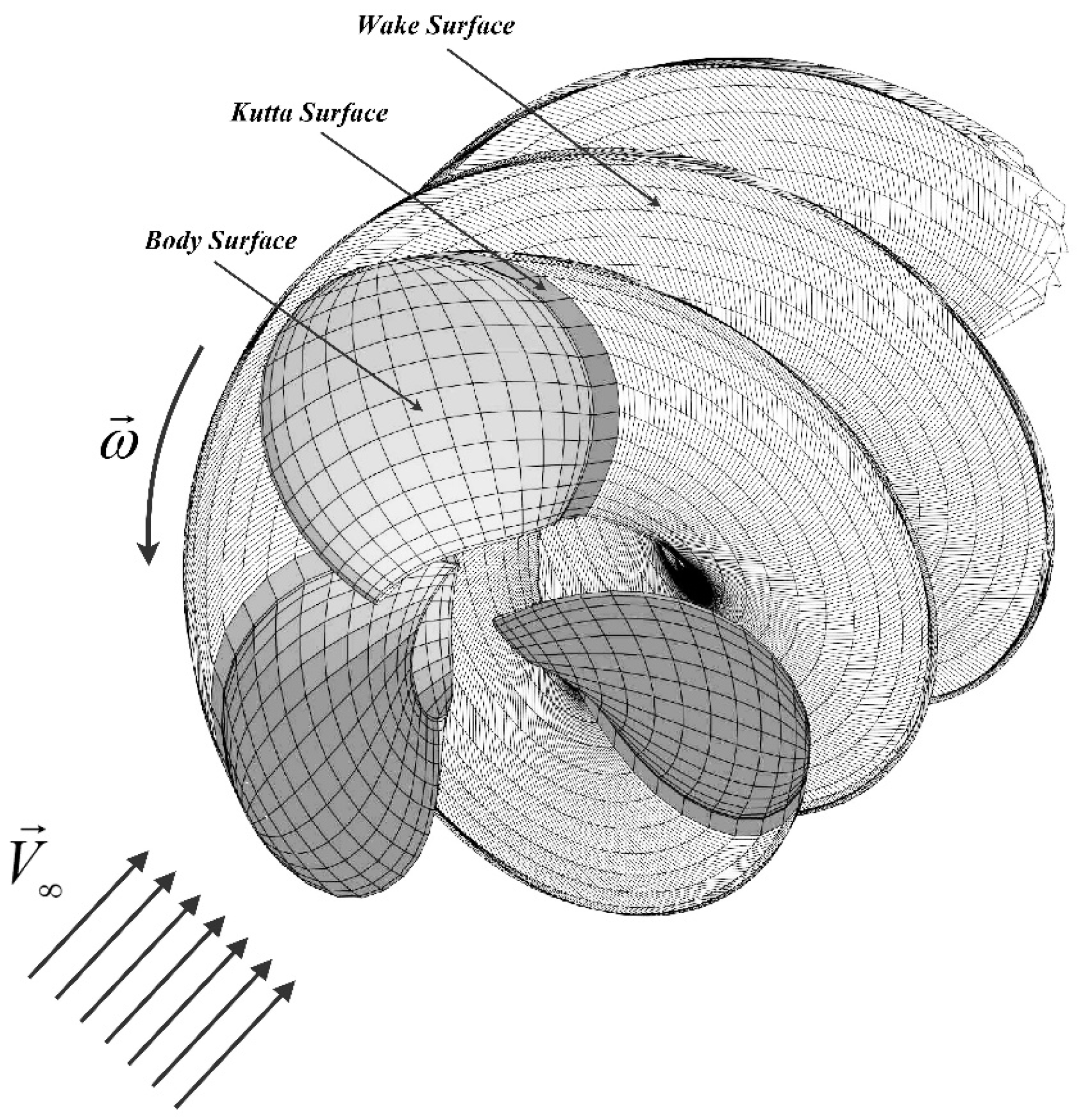
where, surface S includes the body surface, Kutta strip, and wake surfaces, as shown in Figure 1. The control point, source point, and the origin of the coordinate system are represented by P, Q and O, respectively. The vector $\overrightarrow{R}$ is the distance vector between control and source points, and r shows the magnitude of this vector. By supposing ${\varphi }_1=1/r$ and ${\varphi }_2=\varphi$, where $\varphi$ is the potential of flow, ${\varphi }_1$ and ${\varphi }_2$ satisfy the Laplace’s equation [8] and therefore, the left side of Equation (1) will be zero. Then:

$$\underset{S}{\overset{}{{\displaystyle \int }}}(\frac{1}{r}\nabla \varphi -\varphi \nabla \frac{1}{r}).\overrightarrow{n}dS=0.$$

(2)

To avoid singularity in Equation (2), the control point (P) should be excluded from surface S by a small hemisphere of the radius $\epsilon$. Therefore, the surface S will change to $S+S_{\epsilon }$. The value of integral of Equation (2) for $S_{\epsilon }$ is $-2\pi \varphi \left(P\right)$. Then, Equation (2) becomes:

$$\varphi \left(P\right)=\frac{1}{2\pi }\underset{S}{\overset{}{{\displaystyle \int }}}(\frac{1}{r}\nabla \varphi ).\overrightarrow{n}dS-\frac{1}{2\pi }\underset{S}{\overset{}{{\displaystyle \int }}}(\varphi \nabla \frac{1}{r}).\overrightarrow{n}dS,$$

(3)

where, the first and second terms in on the right side of Equation (3) can be interpreted as a dipole (with the strength of $\varphi$) and a source (with the strength of $\nabla \varphi$), respectively. As shown in Figure 1, the surface S is divided into the body surface $\left(S_B\right)$, Kutta strip $\left(S_K\right)$ and wake surface $\left(S_W\right)$. N_B, N_K and N_W represent the number of panels on the body surface, Kutta strip, and wake surface, respectively.

Hence, Equation (3) can re-written as below:

$$\varphi \left(P\right)=\frac{1}{2\pi }\underset{S_B}{\overset{}{{\displaystyle \int }}}(\frac{1}{r}\nabla \varphi -\varphi \nabla \frac{1}{r}).\overrightarrow{n}dS-\frac{1}{2\pi }\underset{S_K+S_W}{\overset{}{{\displaystyle \int }}}(\varphi \nabla \frac{1}{r}).\overrightarrow{n}dS+\frac{1}{2\pi }\underset{S_K+S_W}{\overset{}{{\displaystyle \int }}}(\frac{1}{r}\nabla \varphi ).\overrightarrow{n}dS.$$

(4)

Kutta and wake surfaces have zero thickness and for these surfaces $\nabla \varphi .\overrightarrow{n}=0$. Then, the last term in the right-hand side of Equation (4) becomes zero. This formulation can be interpreted as distributing a source with the strength of $\partial \varphi /\partial n$ on each panel of the body surface and a doublet with the strength of $\varphi$ on each panel of the body surface, Kutta strip, and wake surface. For more simplicity, the strength of doublets on Kutta strip and wake surface is displayed by $\mu$. The final form of Equation (4) is as follows:

$$\varphi \left(P\right)=-\frac{1}{2\pi }\underset{S_B}{\overset{}{{\displaystyle \int }}}\frac{\overrightarrow{n}.\nabla \varphi }{r}dS+\frac{1}{2\pi }\underset{S_B}{\overset{}{{\displaystyle \int }}}\varphi \frac{\overrightarrow{n}.\overrightarrow{r}}{r^3}dS+\frac{1}{2\pi }\underset{S_K}{\overset{}{{\displaystyle \int }}}\mu \frac{\overrightarrow{n}.\overrightarrow{r}}{r^3}dS+\frac{1}{2\pi }\underset{S_W}{\overset{}{{\displaystyle \int }}}\mu \frac{\overrightarrow{n}.\overrightarrow{r}}{r^3}dS.$$

(5)

If the propeller rotates with the angular velocity of $\overrightarrow{\omega }$, and the axial flow velocity introduced into propeller disk is ${\overrightarrow{V}}_{\infty }$ (See Figure 1), the total velocity of point A on propeller blade is:

$${\overrightarrow{v}}_A= {\overrightarrow{V}}_{\infty }+\overrightarrow{r}\times \overrightarrow{\omega }.$$

(6)

The propeller is assumed to be rigid, and the fluid particles cannot enter into the surface of propeller. This boundary condition for all panels of the body surface is [9]:

$${\left(\nabla \varphi .\overrightarrow{n}\right)}_i={\left({\overrightarrow{v}}_A.\overrightarrow{n}\right)}_i i=1,\dots ,N_B.$$

(7)

Then Equation (5) becomes:

$$\varphi \left(P\right)=-\frac{1}{2\pi }\underset{S_B}{\overset{}{{\displaystyle \int }}}\frac{{\overrightarrow{v}}_A.\overrightarrow{n}}{r}dS+\frac{1}{2\pi }\underset{S_B}{\overset{}{{\displaystyle \int }}}\varphi \frac{\overrightarrow{n}.\overrightarrow{r}}{r^3}dS+\frac{1}{2\pi }\underset{S_K}{\overset{}{{\displaystyle \int }}}\mu \frac{\overrightarrow{n}.\overrightarrow{r}}{r^3}dS+\frac{1}{2\pi }\underset{S_W}{\overset{}{{\displaystyle \int }}}\mu \frac{\overrightarrow{n}.\overrightarrow{r}}{r^3}dS.$$

(8)

The value of $\mu$ in the last term on the right-hand side of Equation (8) is obtained from the previous time step. Therefore, the above equation has N_B unknowns for the strength of doublets on body panels and N_K unknowns for doublets on Kutta strip, hence, N_B + N_K unknown totally. Another boundary condition used to solve this problem is the Kutta condition. This condition states that for lifting bodies, the flow smoothly leaves the trailing edge, and the flow velocity should be finite [8]. One of the best ways to apply this condition is presented by Morino [10]:

$${\mu }_i={\left({\varphi }_i\right)}^u-{\left({\varphi }_i\right)}^{l } i=1,\dots ,N_K,$$

(9)

where ${\mu }_i$ is the strength of doublet on Kutta strip i. Also, ${\left(\varphi \right)}^u$ and ${\left(\varphi \right)}^l$ represent the strengths of doublets on upper and lower body panels neighboring Kutta strip i. Kutta conditions will give N_K equations, and N_B equations will be obtained using Equation (8) for all body panels. Finally, by solving this set of N_B + N_K linear equations, all N_B + N_K unknowns will be achieved.

After calculating $\varphi$ on each panel, the total velocity on each panel can be calculated using numerical differentiation methods. Then, unsteady Bernoulli’s equation can be used for calculating the total pressure [11]:

$$\frac{p-p_{\infty }}{\rho }=-\frac{1}{2}{\left|\overrightarrow{\nabla \varphi }-{\overrightarrow{v}}_A\right|}^2+\frac{1}{2}{\left|{\overrightarrow{v}}_A\right|}^2-\frac{\partial \varphi }{\partial t},$$

(10)

where, $\overrightarrow{\nabla \varphi }$ and $\partial \varphi /\partial t$ denote the surface gradient and time derivate of velocity potential, respectively. The propeller thrust can be calculated by integration of pressure forces on panels of the propeller surface. Also, viscous forces $({\overrightarrow{F}}_D)$ should be obtained using empirical formulas for the surface friction coefficient of each panel. Then, the total thrust force $(\overrightarrow{T})$ and torque $(\overrightarrow{Q})$ of propeller are obtained as [12]:

$$\begin{array}{l}\overrightarrow{T}={\displaystyle \int }(p.\overrightarrow{n}+{\overrightarrow{F}}_D)dS\\ \overrightarrow{Q}={\displaystyle \int }\overrightarrow{r}\times (p.\overrightarrow{n}+{\overrightarrow{F}}_D)dS\end{array},$$

(11)

2.1. Validation of Panel Method Code

The DTMB 4119 propeller is one of the propellers which is widely used in modeling and validations of numerical flow solvers. The main particulars and details of the geometry of this propeller are presented in

Table 1. Main Particulars of DTMB 4119 Propeller [13].

Number of Blades	3
Diameter	0.20 m
Blade Sections Profile	NACA 66 modified (a = 0.8)
Design Advance Ratio (J)	0.833

and

Table 2. Geometry of DTMB 4119 Propeller [13].

r/R	c/D	P/D	Skew	Rake	tmax/c	fmax/c
0.2	0.3200	1.1050	0	0	0.2055	0.0143
0.3	0.3635	1.1022	0	0	0.1553	0.0232
0.4	0.4048	1.0983	0	0	0.1180	0.0230
0.5	0.4392	1.0932	0	0	0.0916	0.0218
0.6	0.4610	1.0879	0	0	0.0696	0.0207
0.7	0.4622	1.0839	0	0	0.0542	0.0200
0.8	0.4347	1.0811	0	0	0.0421	0.0197
0.9	0.3613	1.0785	0	0	0.0332	0.0182
0.95	0.2775	1.0770	0	0	0.0323	0.0163
1	0.0800	1.0750	0	0	0.0316	0.0118

. Note that the advance ratio (J) of the propeller is defined as below:

$$J=\frac{V_A}{n.D},$$

(12)

where, n is the rotational speed, and D is the diameter of the propeller.

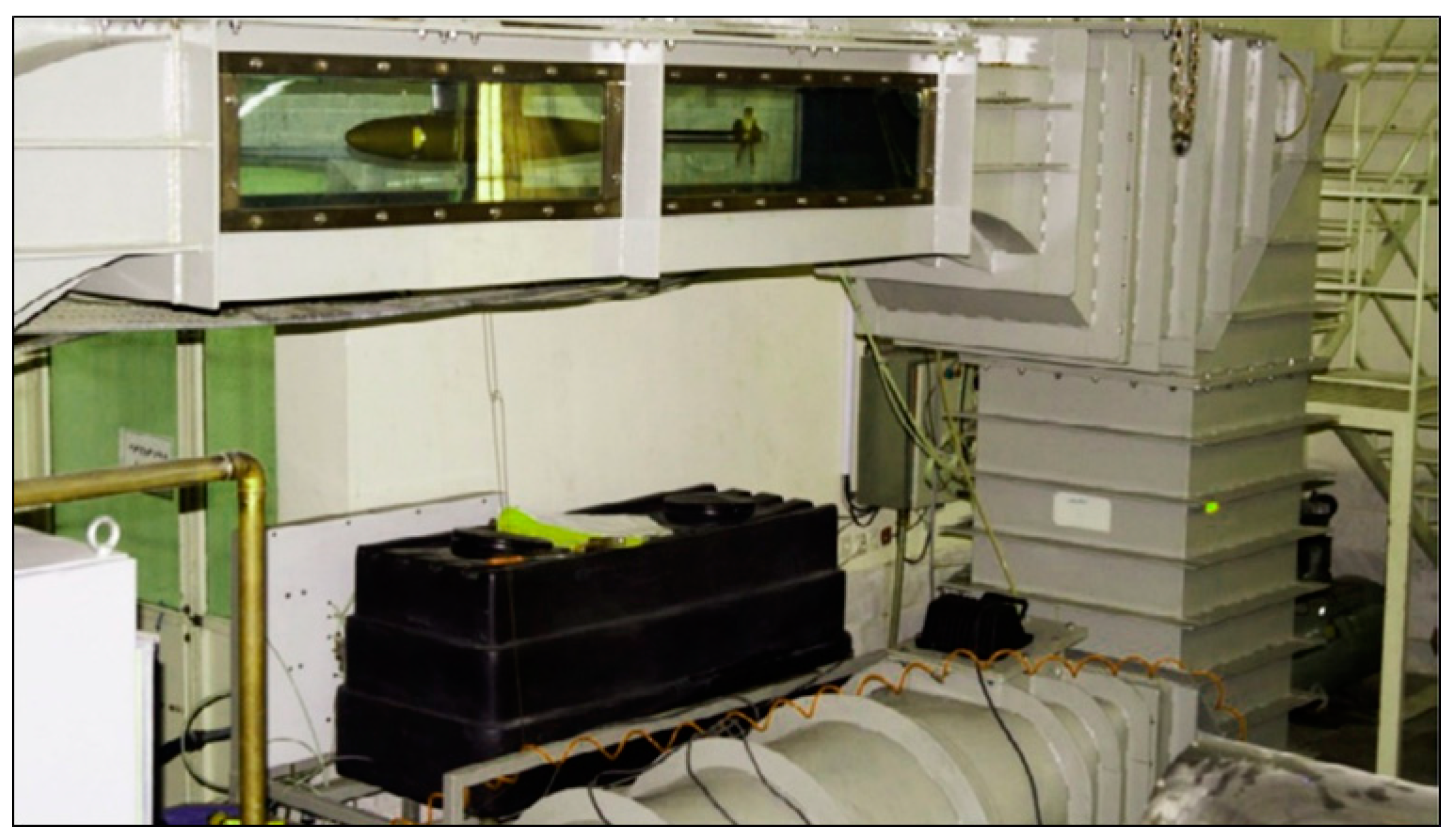
It is more appropriate to use the experimental results of the propeller thrust and torque for validation of results of the panel method code. Accordingly, some experiments were carried out in the cavitation tunnel of the marine engineering laboratory of Sharif University of Technology (Figure 2). In this tunnel, a H29 dynamometer measures the thrust and torque of the propeller, and this data will be used in the validation of numerical results.

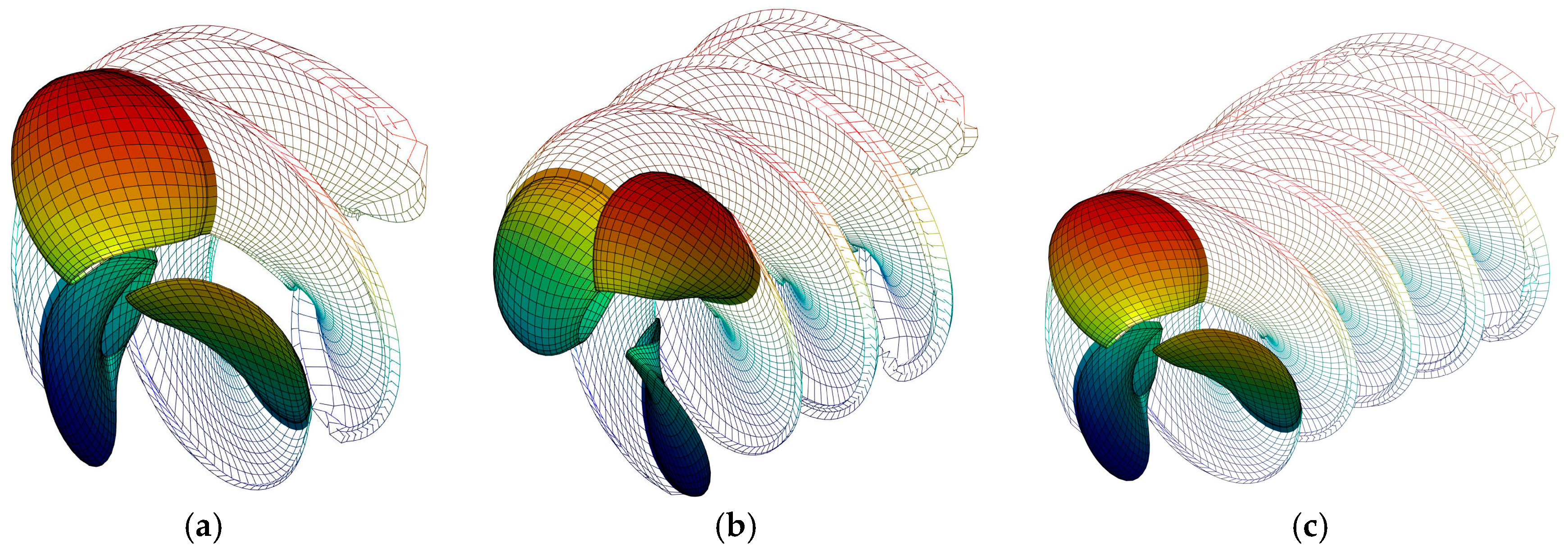
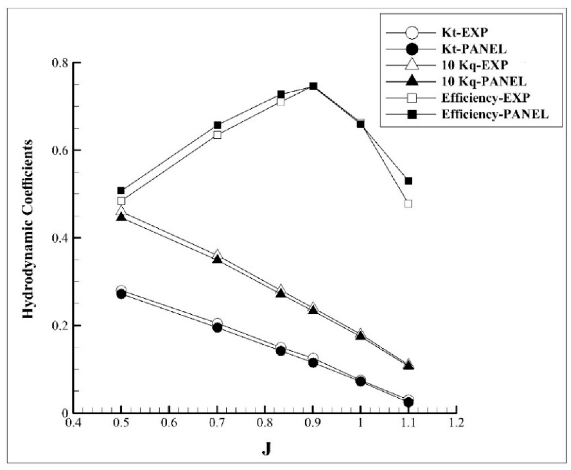
After simulation of the flow around the propeller, wake surface and hydrodynamic coefficients of the propeller (thrust, torque and efficiency) were obtained. Development of the wake surface of the propeller for J = 0.833 at different times is shown in Figure 3. As shown in the figures, the tip vortex of the blades causes a roll-up of the wake surface.

Numerical simulation of the propeller is performed by code developed for various advance ratios, with Figure 4 comparing the hydrodynamic coefficients of the propeller obtained by panel method with experimental data. The thrust coefficient $(K_t)$, torque coefficient $(K_q)$, and efficiency of the propeller $(\eta )$ are defined as below:

$$\begin{array}{l}{K}_t=\frac{T}{\rho n^2{D}^4}\\ K_q=\frac{Q}{\rho n^2{D}^5}\\ \eta =\frac{J}{2\pi }\frac{K_T}{K_q}\end{array}$$

(13)

According to Figure 4, numerical results using the panel method have good agreement with experimental results. The maximum error for the thrust coefficient of propeller calculated by the panel method is 4%, and for the torque coefficient is about 7%. This proves that the accuracy of the panel method is suitable for hydrodynamic performance analysis of marine propellers. One reason for the more significant error of the torque coefficient is the use of empirical formulas when calculating the friction resistance of each panel.

3. Hydro-Acoustic Formulation

One of the most common models for calculating the noise of propellers is the Ffowcs Williams and Hawkings (FW-H) equations. They developed Lighthill equations while considering the rigid body in the flow. For solving the FW-H equations, Farassat et al. [3] presented the integral formulation 1A, which could predict the noise of moving objects. In this formulation, total sound pressure $(p^{\prime })$ is the sum of thickness pressure $({p^{\prime }}_T)$ and loading pressure $({p^{\prime }}_L)$. Thickness pressure is a monopole source, due to the displacement of fluid caused by the movement of blades. Loading pressure is a dipole source, due to the distribution of positive and negative pressures on the face and back of the blade. Quadrupole noise sources have to be neglected because of limitations of formulation 1A and panel method solver, but in general, these sources are not negligible. The above mentioned components are calculated as below [3]:

$$\begin{array}{l}4\pi p^{\prime }{}_T\left(\overrightarrow{x},t\right)=\underset{S}{\overset{}{{\displaystyle \int }}}{\left[\frac{\rho ({\dot{v}}_n+v_{\dot{n}})}{r{\left(1-M_r\right)}^2}\right]}_{ret}dS+\underset{S}{\overset{}{{\displaystyle \int }}}{\left[\frac{\rho v_n\left(r{\dot{M}}_r+c{M}_r-c{M}^2\right)}{r^2{\left(1-M_r\right)}^3}\right]}_{ret}dS\\ 4\pi p^{\prime }{}_L\left(\overrightarrow{x},t\right)=\frac{1}{c}\underset{S}{\overset{}{{\displaystyle \int }}}{\left[\frac{{\dot{L}}_r}{r{\left(1-M_r\right)}^2}\right]}_{ret}dS+\frac{1}{c}\underset{S}{\overset{}{{\displaystyle \int }}}{\left[\frac{L_r-L_M}{r^2{\left(1-M_r\right)}^2}\right]}_{ret}dS\\ +\frac{1}{c}\underset{S}{\overset{}{{\displaystyle \int }}}{\left[\frac{L_r\left(r{\dot{M}}_r+c{M}_r-c{M}^2\right)}{r^2{\left(1-M_r\right)}^3}\right]}_{ret}dS\end{array},$$

(14)

where, $\rho$ represents density, c shows the sound speed in fluid, $\overrightarrow{v}$ is the noise source velocity, $\overrightarrow{r}$ denotes distance vector from the noise source to receiver, $r$ is the magnitude of $\overrightarrow{r}$, Mach number is $\overrightarrow{M}=\overrightarrow{v}/c$, $M_r$ reflects the dot product of $\overrightarrow{M}$ and radiation vector $(\overrightarrow{r})$, $L=p.\overrightarrow{n}$ is pressure force and $p$ is the hydrodynamic pressure. Time derivate of the variables is shown by a dot over the variables. As can be seen, these equations use flow quantities for calculation of noise. Therefore, in the first step, the flow around the propeller should be simulated using numerical methods, such as CFD and BEM. In the current research, the developed code of panel method is used for calculating the flow quantities as input data. Then, according to the receiver in the position of $\overrightarrow{x}$, retarded time $({\tau }_{i,j})$ is obtained for all panels. Finally, all required quantities of Equation (14) (for each panel at the retarded time) must be extracted from input data, numerical integrals of the equation are calculated, and the acoustic pressure of element is obtained. By summing up the acoustic pressures of all elements, a total acoustic pressure is obtained for the specified receiver.

3.1. Validation of FW-H Code

One of the best methods for validation of results of numerical noise codes is measuring the noise in the cavitation tunnel. In this study, experimental tests were carried out in the cavitation tunnel of the marine engineering laboratory of Sharif University. The experimental set-up is displayed in Figure 5.

This method has high accuracy and reliability, but it has complications to be considered. For measuring the noise of a propeller in cavitation tunnel, different procedures and guidelines have been provided by the International Towing Tank Conference (ITTC). The steps of measuring the propeller noise with rotational speed (N) and flow velocity (V) in the cavitation tunnel according to ITTC standards are as follows:

• Measurement of Background Noise (SPL_B): To calculate the net noise of propeller (SPL_N) under different operating conditions, the background noise (from the running facility) of the tunnel must be measured, and correction has to be performed. This step should be carried out by rotating the dynamometer without the propeller at rotational speed N and flow speed of V.
• Measurement of Total Noise (SPL_T): The total noise of the propeller should be obtained by rotating the dynamometer with the model propeller at different operating conditions.

After measuring the background and total noise, the corrections are done based on the difference between noise levels $(\Delta \mathrm{SPL}={\mathrm{SPL}}_T-{\mathrm{SPL}}_B)$ as follows [15]:

• $\Delta \mathrm{SPL}>10$: No corrections;
• $\Delta \mathrm{SPL}<3$: Measurements are dominated by background noise and cannot be used;
• $3\le \Delta \mathrm{SPL}<10$: Corrections should be done by the following expression:

  $${\mathrm{SPL}}_N=10{\log }_{10}\left[{10}^{{\mathrm{SPL}}_T/10}-{10}^{{\mathrm{SPL}}_B/10}\right].$$

  (15)

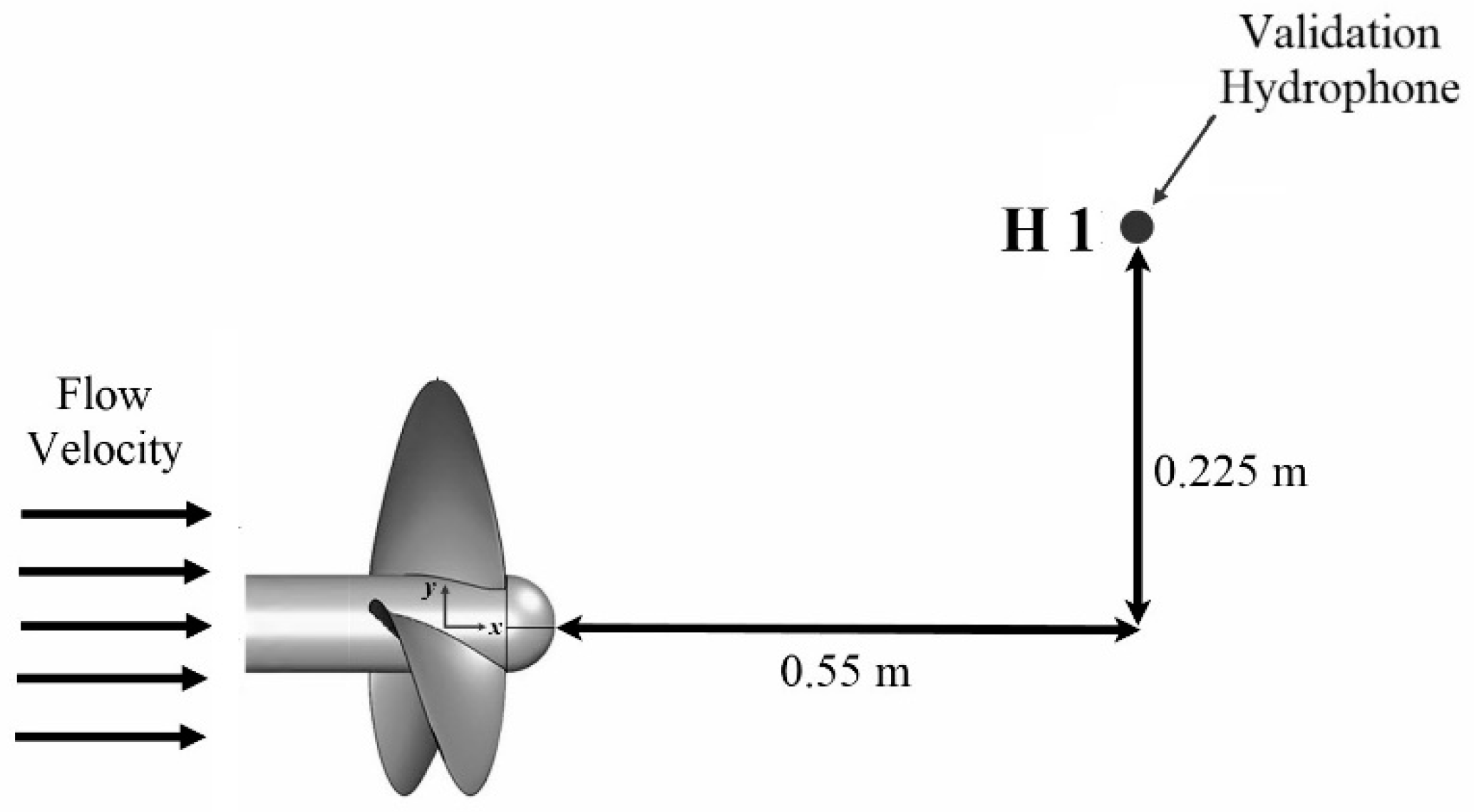
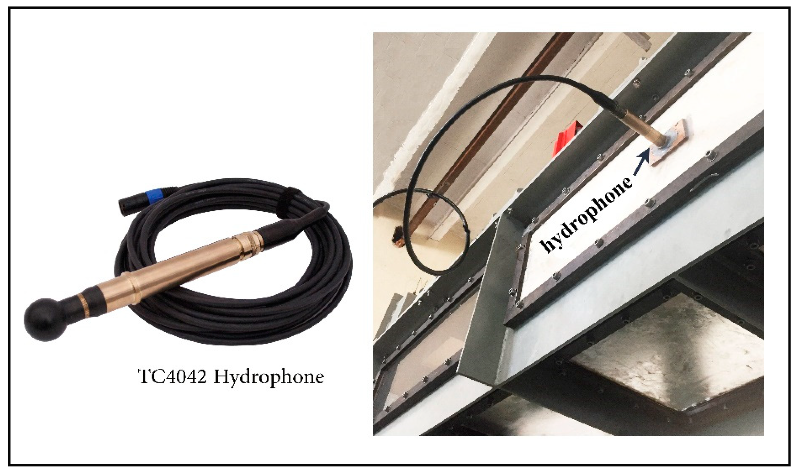
For measuring the noise of the propeller in cavitation tunnel, a Reson TC4042 hydrophone has been used. The distance between this hydrophone and the propeller is given in Figure 6.

Since the experimental results will be used for validation of numerical results of FW-H code, the experimental test conditions are the same as numerical modeling as follows:

• Flow velocity—2.2 m/s;
• Propeller RPM—792;
• Advance ratio (J)—0.833.

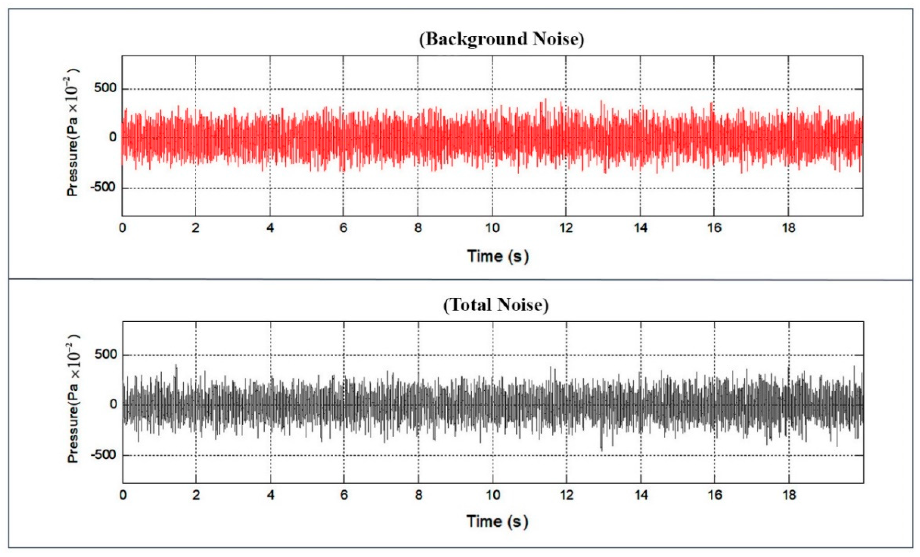
The time history of acoustic pressure recorded by the hydrophone for two states of background and total noise is shown in Figure 7.

In the post-processing step, the Fast Fourier Transform (FFT) was used to transform the acoustic pressure from the frequency domain to the time domain. Next, the following relation was used for conversion of the acoustic pressure into sound pressure level (SPL) [16]:

$$\mathrm{SPL} (\mathrm{dB})=20{\log }_{10}\left(p^{\prime }/p_{ref}\right),$$

(16)

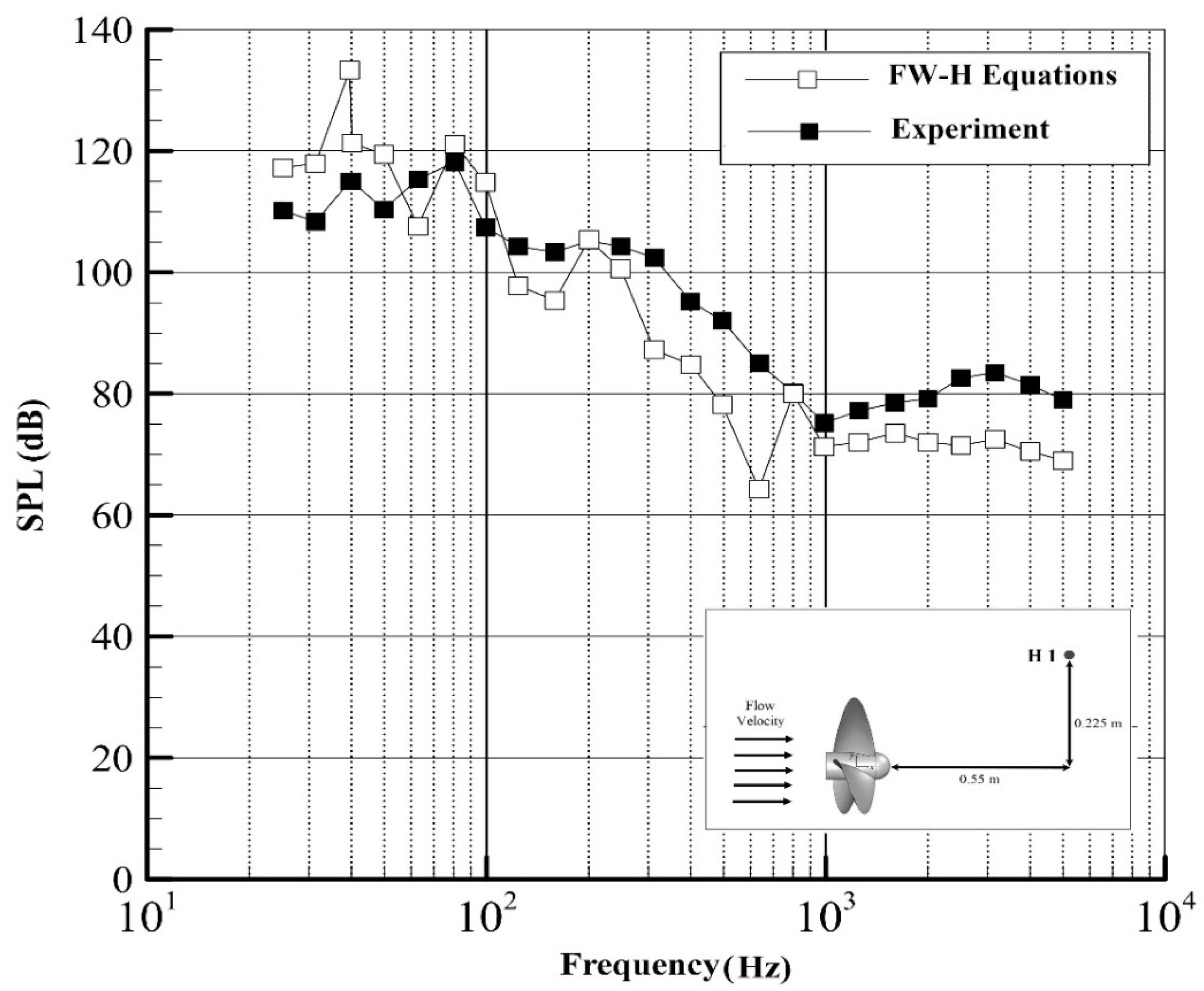
where $p_{ref}$ is the reference pressure and is related to the threshold of a normal human hearing for a frequency of 1 kHz, which is $1 \mathsf{\mu }\mathrm{Pa}$ for water [17]. In this way, the SPL_B and SPL_T will be obtained, and corrections to SPL_T will be made according to ITTC procedures to extract the net noise of the propeller (SPL_N), as described. Figure 8 compares the experimental results of SPL_N with the numerical results of noise calculated by our own developed code. The propeller and flow conditions are the same as the experimental setup.

It can be seen that there is an acceptable agreement between numerical and experimental results, especially within the frequency range of 50 to 250 Hz. The difference between numerical and experimental results in BPF is higher than other harmonics of BPF. Other research [18] carried out on the noise of marine propeller also shows the same results.

One of the most significant sources of error in the numerical results of noise is the error arising from the calculation of pressure and flow velocity by the panel method. As mentioned in the previous section, the panel method has an error of 4 to 7% in calculating the thrust and torque of propellers. Since FW-H equations use panel method outputs, this error can cause inaccuracy in the propeller noise levels. Also, the FW-H equations include some integrals which are evaluated numerically on the surface of the noise source. Note that numerical integration methods have a computational error which can cause an error in the noise values. On the other hand, in the formulation presented for FW-H equation by Farassat, the quadrupole sources of noise are neglected, which could cause a minor error in the propeller noise.

The most important issue in measuring the noise in the cavitation tunnel is the reflection of sound from tunnel walls. This reflection causes an error in the measured noise. Examining the effects of sound reflection requires noise transducer and acoustic tank (without reflection), which unfortunately were not available in our laboratory. The results of research [19,20] carried out in this field show that the reflection of sound in the tunnel can increase or decrease the measured noise level according to the frequency and measurement location in the tunnel. Therefore, another source of error in experimental noise is related to the effects of wall reflections on noise measurement.

As a summary of previous sections, it was observed that the codes developed for simulation of flow around the propeller and calculation of the propeller noise had acceptable accuracy. Accordingly, these two codes can be used further for the optimization of the propeller geometry in terms of noise and hydrodynamic performance. According to the presented analysis, there are differences between the numerical and experimental results. However, the observed accuracy, especially in the range of 50–250 Hz, is considered enough for the purposes of the present study.

4. Genetic Algorithm Optimization of DTMB 4119 Propeller

One of the methods that have been considered in the last two decades to solve optimization problems is the method of genetic algorithm. In this research, a genetic algorithm is used to optimize the hydrodynamic and hydro-acoustic performance of the DTMB 4119 marine propeller. The main geometrical parameters of a marine propeller include radius, the number of blades, rake angle, skew angle, pitch distribution, and chord distribution. Although the radius and the number of blades have a significant effect on the performance of the propeller, variations in the radius do not alter the geometry and only change the scale of the propeller. On the other hand, varying the number of blades generally changes the geometry of the initial propeller. Camber distribution also be one of the geometrical parameters of propellers that the authors decided to study it in future works. Finally, the main geometric characteristics of this propeller investigated in the optimization process are as follows:

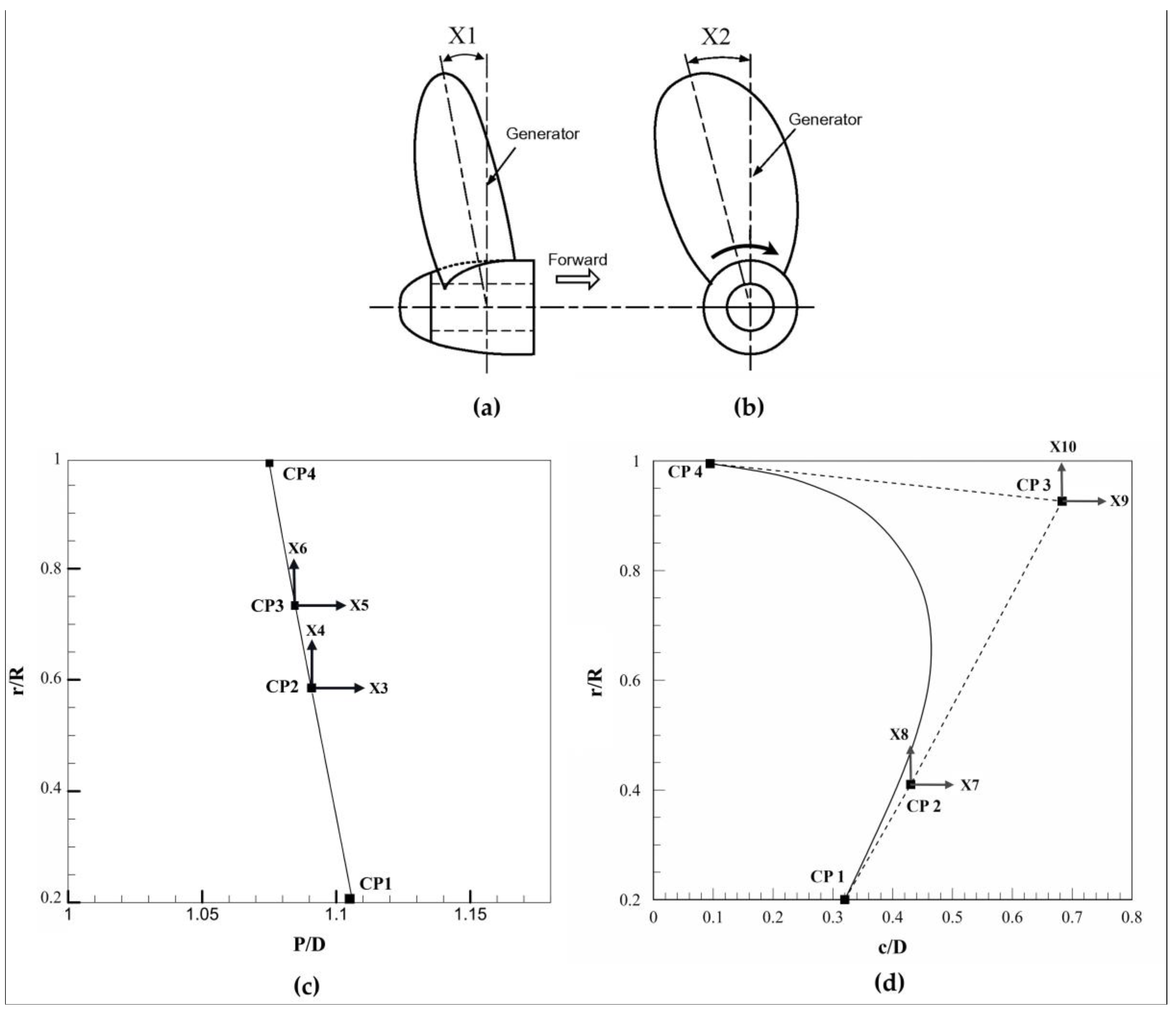
Rake angle: The rake angle is the angle of inclination of the propeller blades relative to the generator line (Figure 9). Rake is one of the main geometric parameters of the ship’s propeller, which has a significant effect on the hydrodynamic and hydro-acoustic performance of the propeller.

Skew angle: The skew angle is defined as the angle between the propeller reference line and a line drawn through the shaft center line and mid-chord point of the last section of the propeller [14].

Pitch distribution: The pitch of a propeller (P) is the distance it would move forward in one revolution. The distribution of a propeller pitch is usually displayed in a dimensionless form of P/D.

Chord distribution: The chord (c) distribution of a propeller is usually displayed in a dimensionless form of c/D.

These characteristics are shown in Figure 9.

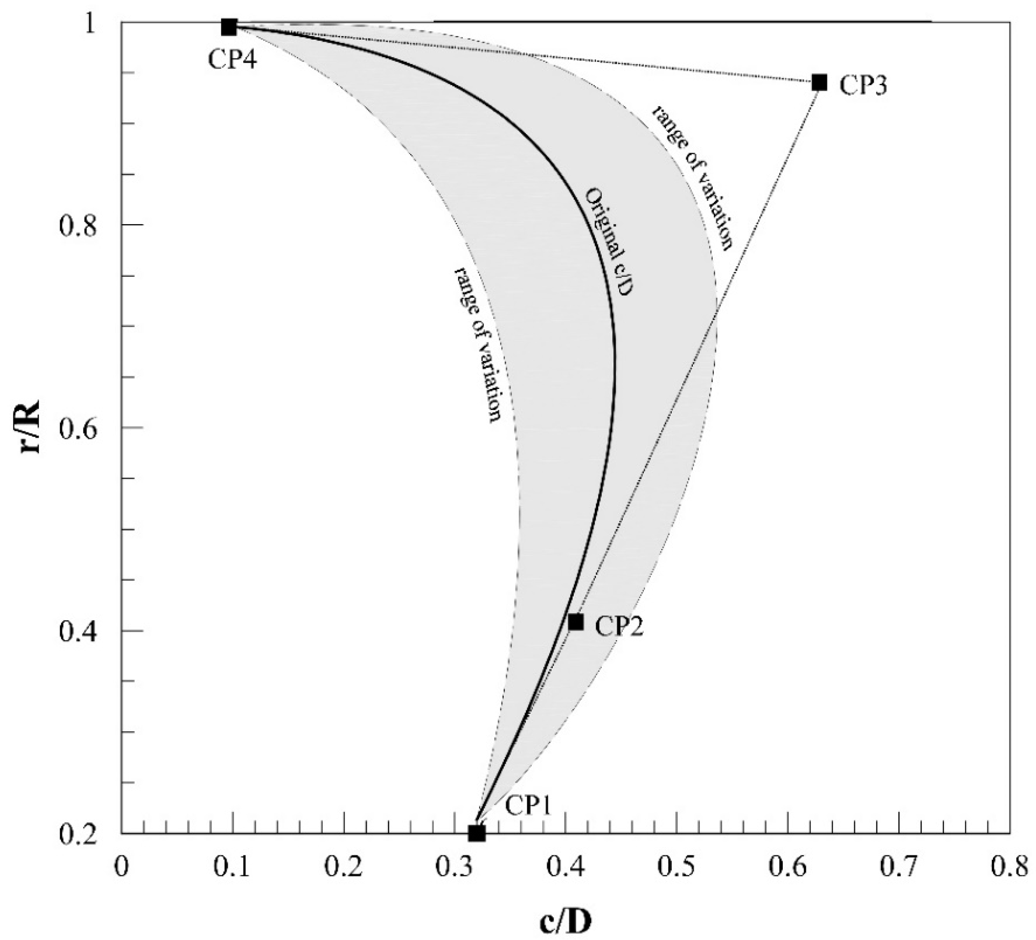
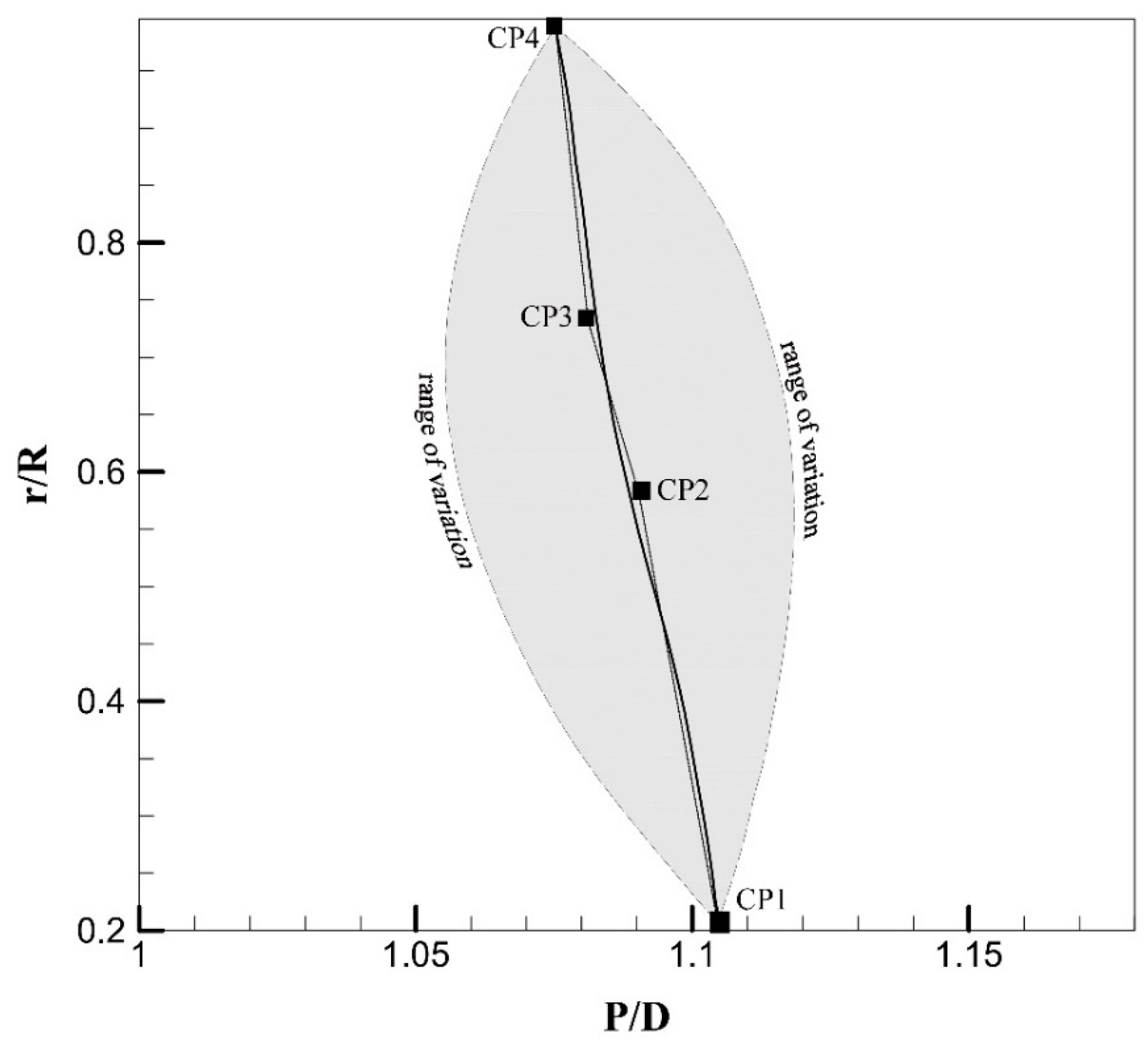
According to the geometry of conventional propellers, the curves of pitch distribution (P/D) and chord distribution (c/D) of propellers are almost smooth and can be represented by B-Spline curves. The B-Spline curve is composed of several control points (CP), where altering the location of these control points will change the curve smoothly [11]. The P/D and c/D curves, as well as the related control points of DTMB 4119 propeller, are shown in Figure 10 and Figure 11, respectively.

In the optimization process, control points 1 and 4 (CP1 and CP4) of the B-Spline curves are assumed to be fixed while control points 2 and 3 (CP2 and CP3) are moved in horizontal and vertical directions. The optimization variables and the range of variations are shown in

Table 3. Optimization variables and range of variations.

Variable		Range of Variations	Variable Name
Rake angle		From 0 to 15 degrees	X1
Skew angle		From 10 to 40 degrees	X2
P/D Curve	Horizontal position of CP2	From −0.04 to +0.04 with step of 0.01	X3
	Vertical position of CP2	From −0.08 to +0.08 with step of 0.02	X4
	Horizontal position of CP3	From −0.04 to +0.04 with step of 0.01	X5
	Vertical position of CP3	From −0.08 to +0.08 with step of 0.02	X6
c/D Curve	Horizontal position of CP2	From −0.06 to +0.06 with step of 0.02	X7
	Vertical position of CP2	From −0.06 to +0.06 with step of 0.02	X8
	Horizontal position of CP3	From −0.15 to +0.15 with step of 0.02	X9
	Vertical position of CP3	From −0.07 to +0.07 with step of 0.01	X10

. According to Table 3, the negative rake angle of the propeller reduces the hydrodynamic efficiency by lowering the thrust force of propeller. For this reason, the negative rake angles are ignored, and the range of variations of rake angle is considered from 0 to 15 degrees with 3-degree steps.

According to data of Table 3, the ranges of variations of P/D and c/D distribution curves for DTMB 4119 propeller are reported in Figure 10 and Figure 11, respectively.

Objective Functions

The design of propellers with a low noise level is of great importance in marine engineering. Therefore, the first objective function in this optimization is to reduce the noise generated by the propeller. As stated in the previous section, the noise level of a propeller in a given location could be calculated by the FW-H equations. In the hydrodynamic analysis of propellers, parameters, such as thrust, torque, and efficiency are of particular importance. The propeller efficiency expresses the ratio of the thrust to the torque of the propeller. Therefore, enhanced efficiency can indicate an increase in the thrust relative to the torque of the propeller. For this purpose, maximizing the propeller efficiency is chosen as the second objective function in optimization. So, the objective functions can be written as follows:

$$\{\begin{array}{l}\mathrm{minimize}:f_1 = \mathrm{SPL}\\ \mathrm{maximize}:f_2=\eta \end{array}.$$

As explained in the earlier sections, the codes developed for flow analysis around the propeller and calculation of the propeller noise could calculate the hydrodynamic efficiency and SPL of the propeller with desirable accuracy. Hence, the output of these codes is used as objective functions.

A Non-Sorting Genetic Algorithm II (NSGA-II) of Mathwork MATLAB 2018 software is used for optimizing the propeller. Given that this code is based on the minimization of objective functions, the increase in the efficiency should be defined by multiplying a negative sign, such as reduction, in the efficiency. According to better accuracy of the SPL numerical results in the frequency range of 50 to 250 Hz, the area under the SPL curve in this range is considered as the objective function. For simplicity, the reduction of noise and the propeller efficiency are expressed as a percentage of the initial propeller noise (A_SPL₀) and propeller efficiency (η₀), respectively. Therefore, the final objective functions are as follows:

$$\{\begin{array}{l}\mathrm{minimize}:f_1=\Delta \mathrm{SP}=\frac{A\_SP{L}_{opt}-A\_SP{L}_0}{A\_SP{L}_0} (\%)\\ \mathrm{minimize}:f_2=\Delta \eta =\frac{{\eta }_0-{\eta }_{opt}}{{\eta }_0} (\%)\end{array},$$

where, subscript opt represents the characteristics of an optimized propeller. $A\_SP{L}_{opt}$ and $A\_SP{L}_0$ are the area under SPL diagram for the optimized and initial propeller, respectively. According to above, reduction of $\Delta \eta$ is equivalent to elevation of the efficiency of the optimized propeller compared to the original propeller.

The thrust (T) and torque (Q) of the propeller are considered as constraints of the optimization. The generated thrust of the propeller must not be less than a specified limit. Moreover, for avoiding overload on the engine, the torque required to rotate the propeller should not exceed a certain amount. Therefore, the thrust and torque constraints on propeller optimization are applied as follows:

$$\{\begin{array}{l}{T}_{opt}\ge T_0\\ Q_{opt}\le Q_0\end{array}.$$

(17)

5. Results

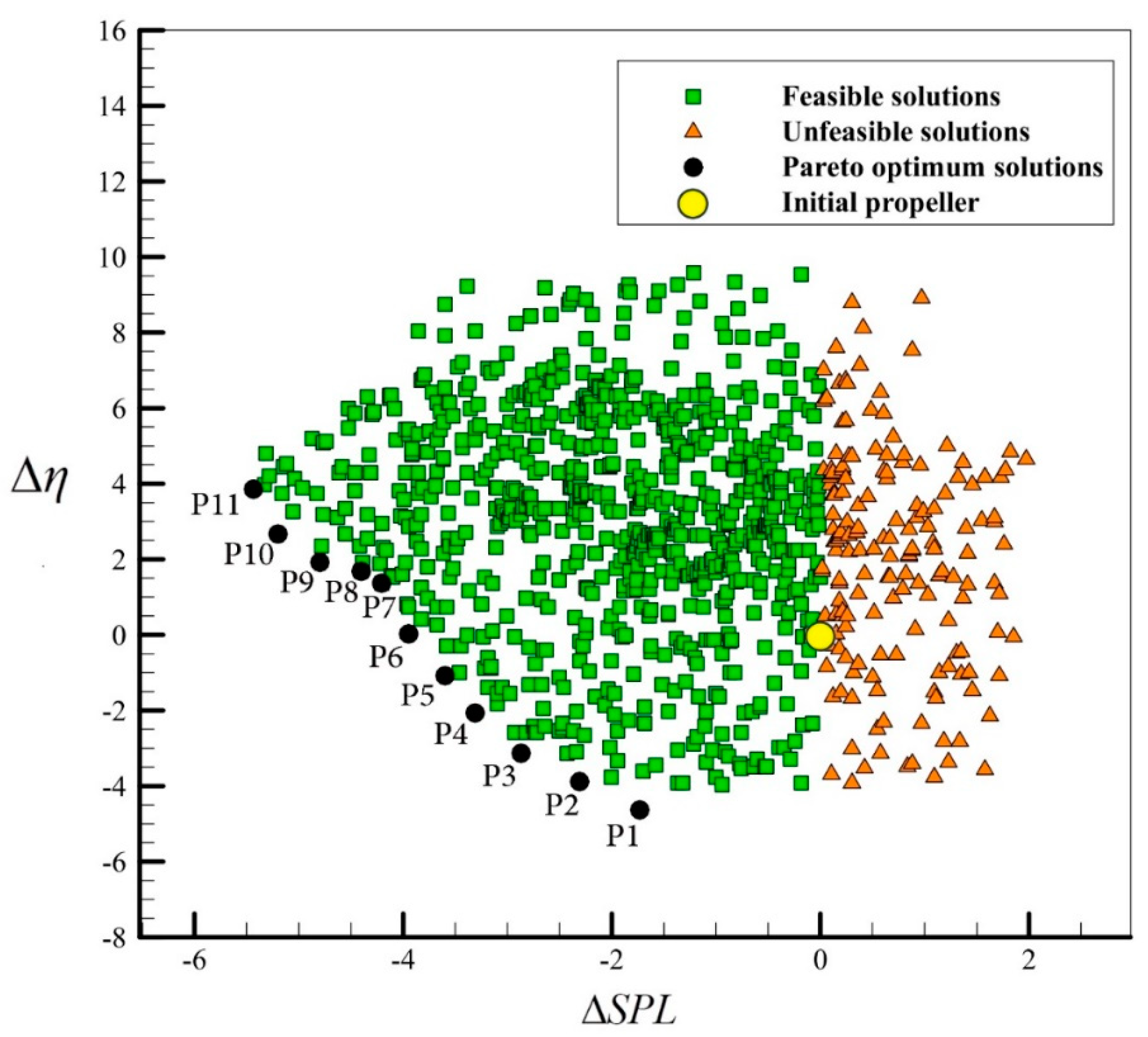
The results of the geometric optimization of DTMB 4119 propeller (original propeller) are summarized in Figure 12. The changes of SPL and efficiency of the original propeller are reported on the horizontal and vertical axes of the diagram, respectively. Pareto optimum solutions include 11 propeller geometries with the values of the objective functions being listed in being listed in

Table 4. The values of objective functions for optimum propellers.

	Pareto Optimal Solutions
	P1	P2	P3	P4	P5	P6	P7	P8	P9	P10	P11
$\Delta \mathrm{SPL}$	−1.73	−2.31	−2.87	−3.31	−3.60	−3.95	−4.21	−4.40	−4.80	−5.20	−5.44
$\Delta \eta$	−4.63	−3.88	−3.13	−2.07	−1.08	0.03	1.37	1.68	1.92	2.67	3.86

.

The values of the rake and skew angles of the optimum propellers are presented in

Table 5. Values of rake and skew angles for optimum propellers.

	P1	P2	P3	P4	P5	P6	P7	P8	P9	P10	P11
Rake	12.05	11.06	10.85	11.36	10.59	9.08	11.25	8.48	9.18	8.14	8.52
Skew	31.52	34.54	33.37	34.52	35.54	38.25	37.85	36.81	37.87	39.74	38.65

. Also, the values of parameters related to the chord and pitch distribution of the optimum propellers are provided in

Table 6. Values of parameters associated with the pitch and chord distribution of optimum propellers.

	P1	P2	P3	P4	P5	P6	P7	P8	P9	P10	P11
X3	−0.02	−0.03	−0.01	−0.02	−0.03	−0.03	−0.03	−0.03	+0.00	−0.02	−0.02
X4	−0.04	−0.02	+0.00	−0.02	−0.06	+0.00	+0.02	−0.04	−0.06	+0.02	−0.02
X5	+0.03	+0.01	+0.02	+0.00	+0.03	+0.04	+0.02	+0.01	+0.04	+0.00	−0.01
X6	+0.08	+0.066	+0.04	+0.04	+0.06	+0.01	+0.02	+0.04	+0.08	+0.04	+0.04
X7	+0.04	+0.06	+0.06	+0.06	+0.02	+0.02	+0.02	+0.04	+0.06	+0.06	−0.02
X8	+0.00	+0.02	+0.00	+0.04	−0.04	−0.02	+0.02	+0.06	+0.06	+0.04	+0.04
X9	+0.09	+0.11	+0.07	+0.11	+0.09	+0.11	+0.05	+0.11	+0.09	+0.07	+0.05
X10	+0.05	+0.07	+0.05	+0.03	+0.04	+0.05	+0.06	+0.02	+0.07	+0.07	+0.05

.

According to results in Table 6, P/D and c/D curves for optimum propellers are shown Figure 13 and Figure 14.

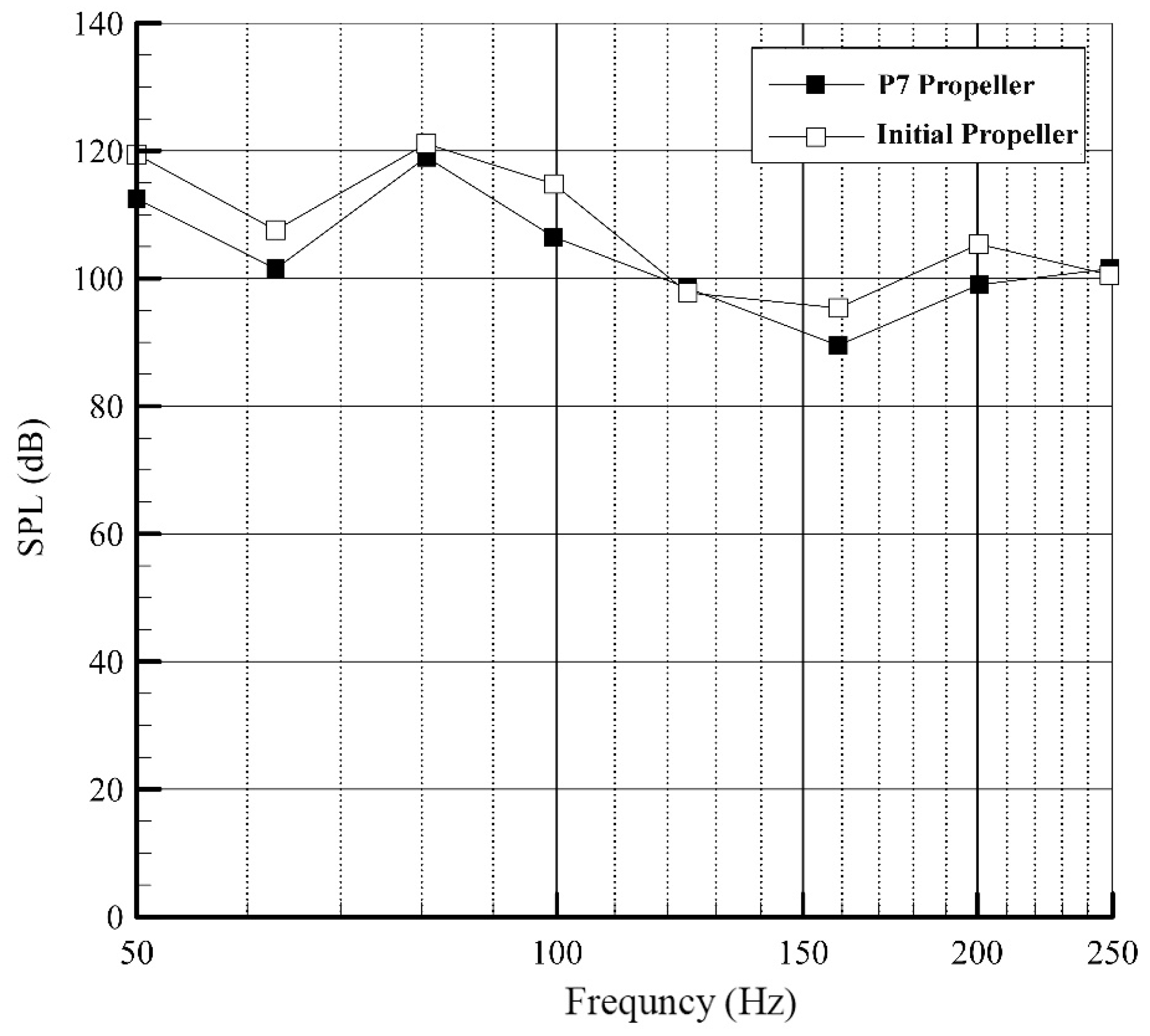
As an example, the diagram of SPL for P7 propeller is compared with the initial propeller in Figure 15.

As shown in Table 5, the optimum geometries have rake angles between 8.14 and 12.05 degrees. In usual, increasing the rake angle increases the thrust, torque, and efficiency of the propeller [21]. On the other hand, increasing the rake, by reducing the difference of pressure on the face and back of the blade, may result in the reduction of propeller noise. Also, increasing the rake angle much than a specific limit may increase the volume of fluid entering the propeller and increase the noise. Therefore, as can be seen in the table of optimum propeller specifications, the rake of all geometries is higher than the initial propeller, although the critical rake angle is about 12 degree. These results suggest that the increase in the rake angle has a critical limit, where values exceeding it do not improve the hydrodynamic and hydro-acoustic performance of the propeller.

Moreover, although the effect of skew is more noticeable in non-uniform inflow mode, the skew angle also affects the performance and noise of the propeller in open water mode because it improves the pressure distribution on the surface of the blade and consequently results in reducing noise and also increasing the propeller efficiency. For this reason, it is observed that the optimum propellers have high skew angles between 31.5 to 40 degrees, which matched the results in References [22,23].

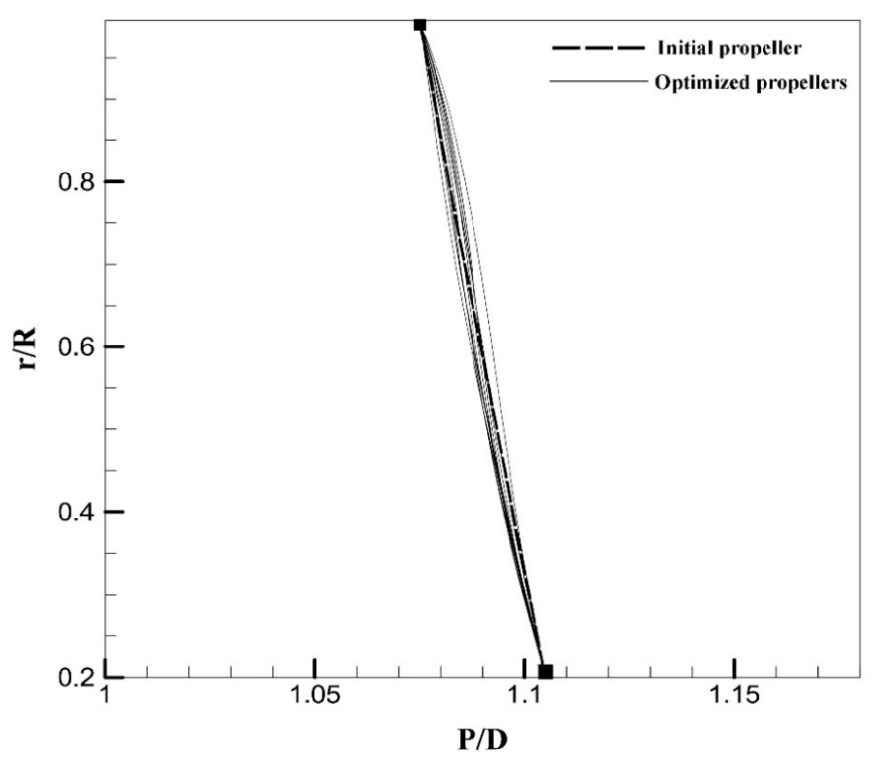
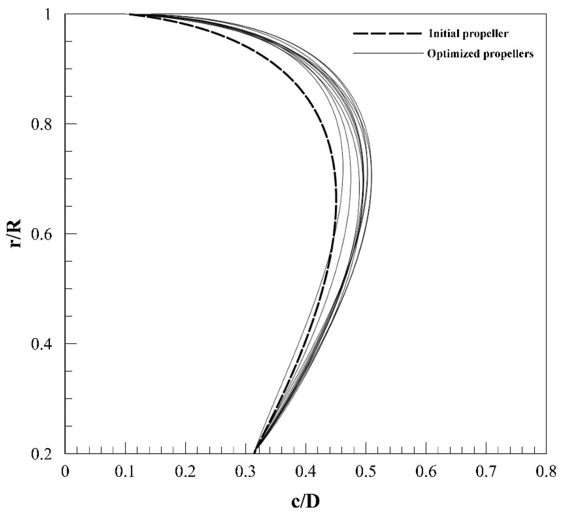
As shown in Figure 13, the P/D curves of the optimized propellers have small variations relative to the curve of the initial propeller. It could mean that the pitch distribution of the initial propeller is nearly optimal. Moreover, as can be seen from Figure 14, the chord of optimized propellers (almost in all r/R ratios) are higher than the chord of the initial propeller. Accordingly, the blade area of optimized propellers is greater than the initial blade $(A_0)$. Therefore, for a specific value of thrust, the pressure difference $(\Delta p)$ between the face and back sides of the blade is smaller. Because, as a general principle, the thrust of propeller is equal to pressure difference on the sides of blade multiplied by the blade area. In the non-cavitation condition, the pressure difference on the sides of the blades is one of the main components of propeller noise (dipole source), which reduces by increasing the c/D.

6. Summary and Conclusions

Marine propellers are one of the most commonly used propulsion systems for ships. In this paper, the geometry of DTMB 4119 marine propeller was optimized by two objective functions, reduction of noise and elevation of efficiency, using a genetic algorithm. The geometric parameters of the propeller, including rake and skew angles, pitch distribution, and chord distribution, were considered in the optimization process. For evaluation of objective functions, a panel method code was developed for modeling the flow around the propeller along with a noise calculation code by solving the FW-H equations. The results of these codes were verified using experimental results obtained in the cavitation tunnel of the Sharif University of Technology. The obtained conclusions are as follows:

▪

For hydrodynamic analysis of marine propeller, the panel method can accurately calculate thrust, torque, and propeller efficiency. The maximum error for the thrust and torque of propeller is 4% and 7%, respectively.

▪

Calculation of the propeller noise using FW-H equations has a good agreement with experimental results in the frequency range of 50 to 250 Hz, while differences are observed at BPF and for frequencies higher than 250 Hz. The reasons for these differences may be related to errors and simplifications of the numerical method, e.g., the assumption of negligible quadrupole noise, and measurement issues, such as the reflections of sound from tunnel walls.

▪

By optimization of the propeller using a genetic algorithm, 11 optimum geometries are obtained as Pareto optimal solutions.

▪

The optimum geometries have rake angles between 8.14 to 12.05 degrees. Increasing the rake angle, by reducing the difference of pressure on the face and back of the blade, may result in the reduction of propeller noise. Therefore, as can be seen in the table of optimum propeller specifications, the rake of all geometries is higher than the initial propeller, although the critical rake angle is about 12 degree.

▪

The optimum propellers have high skew angles between 31.5 to 40 degrees.