Abstract
This paper evaluates the applicability of the hexahedral block structured grids for marine propeller performance predictions. Hydrodynamic characteristics for Potsdam Propeller Test Case (PPTC), namely thrust and torque coefficients, were determined using numerical simulations in two commercial solvers: Ansys Fluent and STAR-CCM+. Results were attained for hexahedral and tetrahedral hybrid grids equivalent in terms of cell count and quality, and compared to the experimental results. Furthermore, accuracy of Realizable k- and SST k- turbulent models when analyzing marine propeller performance was investigated. Finally, performance characteristics were assessed in cavitating flow conditions for a single advance ratio using Zwart–Gerber–Belamri and Schnerr and Sauer models. The resulting cavitation pattern was compared to cavity extents and shape noted during measurements. The results suggest that hexa and hybrid grids, in certain range of advance ratios, do provide similar results; however, for low and high ratios, structured grids in conjunction with Realizable k- model can achieve more accurate results.
1. Introduction
Propellers are an essential component in ship propulsion. They vary in shapes and sizes depending on the load and required performance. Their primary purpose is to convert rotational velocity into useful thrust. Since their inception, marine propellers have been subjected to iterative improvements. This has resulted in a plethora of different designs for various use cases. Initially, the only viable option for propeller performance analysis was the model basin test. With time, first empirical models have been formulated enabling engineers to predict performance characteristics of modified propeller designs without the need to conduct experimental tests. This approach, though convenient, did not always yield correct results, urging the development of alternative techniques [1].
One of the oldest numerical methods for propeller behavior ascertainment is Blade Element Theory (BET) [1,2]. The principle approach includes blade decomposition, force evaluation for each segment and subsequent integration across the entire blade. With the introduction of the momentum theory, certain deficiencies of BET were mitigated. This coupled method is known as Blade Element Momentum Theory (BEMT). Recently, Integral Boundary Layer Method (IBLM), a modified BET implementation, was analyzed by Benini [3]. The method demonstrated good agreement with experimental data when predicting propeller behavior near the working point. Unfortunately, outside of the optimal range, errors in predictions were significant.
The panel method, an implementation of the Boundary Element Method (BEM) in fluid mechanics, is the prevailing industry standard; the method is thoroughly evaluated, simple to implement and sufficiently accurate in propeller performance predictions in both cavitating and non-cavitating conditions [4]. However, even though the method tends to be very efficient, this is not necessarily always true. Furthermore, physically erroneous results can be obtained for certain flow types [5]. An apparent alternative is the viscous flow model, which, due to its complexity and high computational requirements, for a long time, was not suitable for general use. Nowadays, however, propeller Computational Fluid Dynamic (CFD) analyses can be done quickly and efficiently, with results comparable to the experimental data [6]. Considering that the fluid motion in most real-world conditions is case specific, industrial application of CFD relies on proper implementation of turbulent models tailored for the designated case. Despite being the most accurate, Direct Numerical Simulations (DNS) are usually avoided due to excessive computational times and requirements linked to turbulence solving across all scales. Large Eddy Simulations (LES) show potential [7]; however, they are still computationally too demanding and require time, which is scarce in a heavily iterative processes in industrial conditions. Reynolds-averaged Navier–Stokes (RANS) based turbulent models, therefore, are the most common. They employ averaging methods to simplify turbulent flows. RANS models are robust, comparatively simple and can provide acceptable results for engineering applications in limited time frames.
The validity of BEM for both ducted and open propellers was evaluated by Baltazar and Bosschers [8]. As expected, the method was able to predict performance characteristics reasonably well for open propellers; however, the results for ducted models showed discrepancy between experimental data and numerical results. Consequently, RANS analysis was suggested as a potential alternative. In their latest study, Baltazar et al. [9] employed RANS in order to improve and optimize current BEM methodology. BEM applicability when analyzing cavitation was explored by Pereira et al. [10]. The results show that BEM has the ability to predict sheet cavitation accurately; however, modeling viscous flow and tip vortices was unfeasible. A comparison of BEM and RANS methods was conducted in several studies [4,6]. The authors concluded that both approaches have merit; BEM, thanks to its simplicity and robustness can be used for general blade design, whereas RANS usually provides better results, especially at lower advance ratios where viscous effects are pronounced, but at a higher computational cost. The coupled BEM–RANS model was investigated in [11,12] for cavitating and non-cavitating conditions, where RANS methods were used for viscous flow analysis, namely wake and velocity fields, with respect to propeller forces calculated using BEM.
Purely RANS approach in the context of propeller performance predictions has been extensively assessed over the past decade with the two-equation k- turbulence model as the most frequent model of choice [13]. The studies by Bhattacharyya et al. [13] and Krasilnikov et al. [14] utilized unstructured grids and focused on current scaling approaches with SST k- turbulence model as a validation and development tool. Simpler algebraic and one-equation models are rarely used, and, if so, only for preliminary tests. The Reynolds Stress Model (RSM) investigated by Morgut and Nobile [15] showed minor improvements in predictions when compared to SST k- model. The transition Sensitive Turbulence Model (TSM) evaluated by Wang and Walters [16] was able to predict performance characteristics with error margins. Consequently, common two-equation models were preferred considering lower computational times. Helal et al. [17] analyzed cavitation using k- and TSM models and concluded that both could be effective, depending on the advance ratio. Delayed Detached Eddy Simulation (DDES) utilized by Viitanen et al. [18] delivered acceptable results, thus, for open water tests, it was deemed unnecessary, whereas, for cavitating flows, perceivable improvements over common RANS methods were noted. A comprehensive study on cavitation was done by Vaz et al. [5] with summarized results showing the potential of RANS models; however, a preferred method was not presented. Recently, Tu [19] evaluated the applicability of different grids and RANS models for marine propeller performance predictions.
Marine propellers can exhibit various degrees of skewness with pronounced curvatures along the edges and the blade tip. Resulting geometric complexity presents a challenge when generating quality hexahedral block structured grids (hereinafter, structured grids), thus making tetrahedral hybrid unstructured grids (hereinafter, unstructured grids) a de-facto standard. Only a handful of studies tried to analyze and correlate grid type and prediction accuracy. Significance of structured grids when predicting open water characteristics was investigated by Da-Qing [20]. The results were within of experimental data, while grid sensitivity study showed only minor correlation between grid size and results. Some studies [15,21] concluded that similarly sized structured and unstructured grids could achieve equivalent levels of accuracy. As a result, unstructured grids were accepted as a better choice because they are easier to generate. However, Morgut [15] also highlighted the problem of greater diffusivity in unstructured grids and recommended the use of structured grids for local flow studies.
In this study, pertinency of different RANS and cavitation models for industrial use was investigated, with a focus on hexahedral structured grids and their advantages. The objective was to define a proper methodology in marine propeller performance analysis, which, regardless of the solver in use, should provide adequate propeller open water and cavitation characteristics. Ultimately, the presented approach could serve as a baseline for further oblique flow analyses as well as ducted and inclined propeller studies.
2. Methodology
2.1. Geometry and Grid Generation
VP1304 is a five-bladed controllable pitch propeller, a test propeller experimentally validated by SVA Potsdam. Experimental data are publicly accessible under the name Potsdam Propeller Test Case (PPTC) [22] and were used throughout the course of this study. Open water tests were conducted in a 250 m × 9 m × 4.5 m towing tank with propeller submerged at , where D represents the diameter of the propeller. Cavitation analysis was done in K15A cavitation tunnel with 0.6 m × 0.6 m cross section. Relevant forces and torques for latter were determined with a dynamometer placed in front, while, for the former, measurement was done behind the propeller. All results were corrected with dummy hub measurements to minimize extrinsic influences [22].
PPTC VP1304 can be classified as a heavily skewed propeller, especially when compared to traditional test case propellers such as INSEAN E779A [5,23]. It is characterized by a diameter of 0.25 m, mean pitch ratio of and an effective skewness angle of . Since VP1304 is a controllable pitch propeller, a slight gap exists between the blade and hub; to simplify grid generation, this gap was removed. Complex geometry, especially around the blade tip, presents a challenge when generating structured grids, causing the creation of highly skewed and twisted elements. Therefore, considerable attention was attributed to proper mesh generation around the tip area.
For both open water and cavitation tests, several coarse and fine structured grids were created. Since forenamed tests differed in hub geometry and methodology, this was necessary, even though the blade itself remained unchanged. Domain size was kept the same, as well as the general approach to the grid generation. To further augment our results, several unstructured grids were created, the results of which were compared to their structured counterparts with similar quality and cell counts. An overview of discussed computational grids is given in Figure 1.
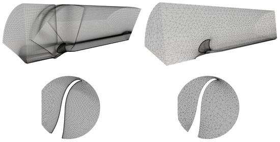
Figure 1.
Computational grids and cell distribution at the blade center: structured grid (left); unstructured grid (right).
To ensure grid integrity despite scaling, cell spacing around the edges and blade tip was kept small. Moreover, as shown in Figure 2a, structured grids were further refined on the upper part of the blade. These areas tend to be of utmost importance when evaluating performance and analyzing cavitation. Boundary layer was fully resolved with 41 grid layers and dimensionless wall distance enforced throughout all the tests. Orthogonal quality and skewness were in acceptable ranges with occasional outlier cells. Full geometric representation was achieved for all structured grids. To attain comparable levels of grid uniformity while maintaining similar cell count, the number of grid layers for preliminary unstructured grids was limited to 20. Further increase led to severe distortions of tetrahedrons, which deemed the validity of the results questionable. Nonetheless, unstructured grids with 41 layer were also evaluated and incorporated additional refinements around the blade. Details of radial sections at m shown in Figure 2a,b indicate certain dissimilarities in generated grids. Based on verified geometry congruity, this discrepancy can be attributed to mesh generator’s interpretation of significant facets and edges. Importance of this differences, however, is negligible, as is demonstrated in subsequent sections.
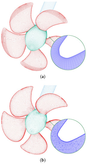
Figure 2.
Grids with ≈ cells used for open water calculations with radial cross sectional detail at m: structured grid (a); unstructured grid (b).
2.2. Numerical Model
One of the goals of this study was to establish a proper approach to CFD analysis of a marine propeller. Fundamentally, nearly all propeller CFD analyses have the following in common: a certain type of grid is generated; depending on the problem, the grid is further refined and subsequently analyzed using an appropriate flow model. Accuracy of these results prominently relies on adequate geometry representation and grid sensitivity in key regions, whereas the choice of the turbulent model, if the mesh is properly defined, has less of an impact. However, in certain circumstances, adopting a proper flow model can be instrumental in obtaining valid results.
Navier–Stokes equations are a set of coupled partial differential equations, namely continuity, momentum and energy equations, that, under the assumption that the fluid acts as a continuum, describe the incompressible fluid flow. They are challenging to solve and are therefore usually simplified using approximations. Among all approaches, Reynolds–averaged Navier–Stokes models are still the only viable option for industrial use where evaluation time is a key factor and absolute accuracy ordinarily is not required. To solve the Navier–Stokes equations, RANS models use a method called Reynolds averaging in which flow variables are obtained as a result of time or ensemble averaging [24]. In Cartesian coordinates, averaged isothermal momentum and continuity equations can be written as:
where are the Cartesian coordinates, are components of the velocity in Cartesian coordinates, t is the time, p is the pressure, represents density, is the viscosity coefficient, stands for stress term called Reynolds stresses and is the Kronecker delta.
To close these equations, Reynolds stresses needs to be properly modeled. RANS turbulence models propose several different approaches; however, for marine propeller analysis, two equation k- and k- models are commonly used. In this study, both Realizable k- and SST k- models were evaluated.
2.3. Numerical Setup
The generated computational domain has a cylindrical shape with a diameter of , where D represents the diameter of the propeller. The cylinder extends up to in upstream and in downstream direction with respect to the blade center. The proposed domain size achieves balance between theoretical requirements and evaluation time.
Recent studies have been utilising [15,25,26] or [27,28] as the domain upstream size in order to achieve inflow uniformity. Downstream lengths usually vary and are based on an approximations of a fully developed flow. Consequently, values larger than are usually adequate. Cross-section is almost exclusively circular with an average diameter of ; however, some studies employ values larger than [15,25,27,28,29]. Given that the experimental measurements were conducted with a propeller submerged at , this seems unnecessary.
Figure 3 illustrates the computational domain. Domain size and shape are preserved for both open water and cavitation tests. Cross-sectional difference between employed CFD model and cavitation tunnel is . Consequently, mean inflow velocity used in cavitation tests was corrected to account for physical restriction. Due to the periodic nature of marine propellers, single passage was extracted and analyzed, significantly reducing required computational time.
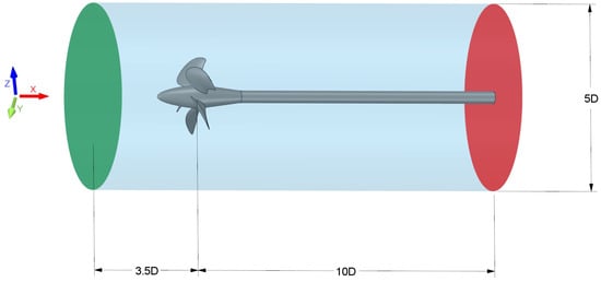
Figure 3.
Size and shape of the computational domain for open water numerical simulations.
Boundary conditions were chosen and set so as to replicate open water tests and tests in the cavitation tunnel. Rotational speeds for open water and cavitation tests were set at s and s, respectively. They differ from the experimentally noted values at worst by . Consequently, this discrepancy was deemed negligible. On the inlet boundary, uniform inflow was assumed and therefore constant velocity with turbulence intensity of prescribed. Turbulence intensity was estimated based on the calculated Reynolds values for external flow. On the outlet boundary, static pressure was specified. Normal velocity component on the outer wall was assigned a zero value Dirichlet boundary condition, whereas tangential velocity utilized Neumann boundary condition, implying it can assume a non-zero value. This boundary condition is commonly known as free-slip. Shaft, hub and blade walls have no-slip condition imposed, meaning both tangential and normal velocity components make use of Dirichlet boundary condition. Remaining faces ensure rotational periodicity and coincide at an angle of along the horizontal axis. Adopted boundary conditions are well established in the field [15,25], however, some disparities in approaches do exist, namely with regards to free-slip walls and outlets [5,6,23]. An overview of applied boundary conditions is given in Figure 4.
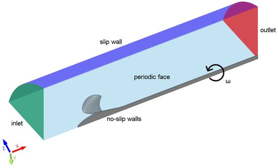
Figure 4.
Prescribed boundary conditions for open water calculations.
Numerical results presented in this study were obtained using two commercial finite volume based CFD solvers: Ansys Fluent and STAR-CCM+. Their dominance in the industrial CFD market is the main reason they were validated for these marine propeller analyses. Both employ a segregated solver with SIMPLE algorithm to couple pressure and velocity fields. Second-order discretization schemes were used predominantly, except for volume fraction in cavitation tests, where HRIC scheme was utilized. Convergence was assumed if variance for both thrust and torque throughout the last 1000 iterations was less than of their mean values or if residuals for all variables fell below . To replicate the rotational behavior of a marine propeller, as well as strike balance between accuracy and evaluation time, Single Moving Reference Frame (SRF) approach was implemented. Transient solutions for open water tests, although more accurate, are of less importance, since those results eventually need to be averaged in order to obtain mean thrust and torque values required for open water curves. For cavitation predictions, transient evaluation was conducted in order to achieve realistic results.
2.4. Hydrodynamic Theory of a Propeller
Hydrodynamic characteristics are a series of dimensionless coefficients that define relative performance of a propeller with respect to its mechanical properties and properties of the fluid. These coefficients are defined so as to facilitate comparison between different types and sizes of propellers. Thrust and torque are expressed as thrust and torque coefficients:
where T is the thrust, Q is the torque, D is the diameter of the propeller, n is the rotational speed of the propeller and is the density of the fluid. Furthermore, a dimensionless coefficient known as advance ratio J is used to express the ratio between the speed of the propeller and propeller tip speed:
Finally, open water efficiency of the propeller can be calculated as:
These coefficients are commonly imparted using open water diagrams, which correlate the speed of the propeller, by means of the advance ratio, with relative thrust, torque and efficiency.
2.5. Grid Sensitivity Study
Open water grid sensitivity study was conducted for . This advance ratio was chosen as it corresponds to the midpoint of the analyzed advance ratio range. The number of elements in the created structured grids is , , , , and , respectively. As previously stated, grids were generated using scaling factors with dimensionless wall distance . Tests were conducted in Fluent using Realizable k- turbulence model. Discrepancies between numerical results and experimental data for open water and subsequent cavitation tests are expressed as relative errors:
Relative errors in thrust coefficient predictions are below for the majority of the grids. Torque coefficient is overpredicted and generally exhibits errors below . The smallest grid, as expected, achieves the lowest accuracy, with errors near for torque and for the thrust coefficient. Increase in grid size leads to a steady convergence, with the largest grid achieving the best overall predictions. However, utilizing a grid with cells for multiple CFD analyses is not practical. Given the fact that the errors for all cases are low, grid with ≈ cells is chosen as the cornerstone of our study since it provides significant savings in computational time while offering acceptable results. Relative errors for different grids are shown in Figure 5.

Figure 5.
Relative errors in performance predictions for grids used in open water grid sensitivity study, Fluent.
Cavitation sensitivity study was conducted for freestream inflow velocity and cavitation number using STAR-CCM+. This corrected velocity accounts for cavitation tunnel blockage and allows the use of previously described open water boundary conditions for a differently sized domain. The resulting advance ratio is . Generated grids are comprised of , , , , , and cells. Errors in torque predictions are well below , with thrust prediction errors settling around throughout most of the tests, as can be seen in Figure 6. Despite these errors, numerical simulations converged well, thus, analogously to open water tests, grid with ≈ cells was similarly deemed acceptable for cavitation analysis.
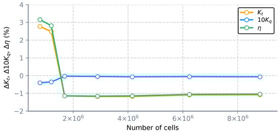
Figure 6.
Relative errors in performance predictions for grids used in cavitation grid sensitivity study, STAR-CCM+.
3. Results and Discussion
3.1. Open Water Performance
Open water tests were conducted with the same hexahedral block structured grids in both solvers for advance ratios ranging from to , with rotational velocity set at s. SST k- model was initially adopted for performance assessment in Fluent and STAR-CCM+. The results of these tests for structured grids are shown in Figure 7.
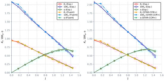
Figure 7.
Comparison between experimental measurements and CFD results for structured grid attained with k- model in: Fluent (left); STAR-CCM+ (right).
Both solvers exhibit comparable levels of accuracy overpredicting coefficients at lower and underpredicting them at higher advance ratios. In general, Fluent provides more consistent results and for higher advance ratios gives better overall predictions. For bollard pull condition (), torque coefficients are equivalent. Thrust is overpredicted in STAR-CCM+ and underpredicted in Fluent by a similar percentage. Across the majority of tests, relative difference between CFD results and experimental measurements is below for thrust and for torque. Significant discrepancies are observed for thrust predictions at where Fluent deviates by and STAR-CCM+ by , which is somewhat expected, since similarly erroneous discrete values at lower absolute thrusts and torques will result in higher relative errors.
The preliminary unstructured grids (Figure 1) deliver similar results in both solvers when using SST k- model. However, when compared to structured grids and experimental measurements, they underestimate torque and thrust coefficients up to at lower advance ratios, which can be attributed to diffusive errors common to those grids as well as potentially unresolved viscous sublayer. Additionally, predicted values tend to oscillate, which calls into question the validity of results. Errors for highest advance ratios are comparable and around . Realizable k- model provided marginally worse results for unstructured grids when compared to SST k- model; on average, coefficients are further overpredicted by , while for lowest advance ratios this disparity is . The comparison between experimental measurements and results for unstructured grids using different two-equation turbulent models is shown in Figure 8.
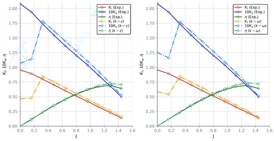
Figure 8.
Open water results for unstructured grids using: Realizable k- (left); SST k- model (right).
Due to imposed limitations in cell count, unstructured grids were not able to fully capture the blade profile, which is substantiated by pressure fluctuations along the blade sections (Figure 9). It can be reasonably assumed that cumulative numerical errors led to the minimization of disparities between CFD results and measurements for core ranges.
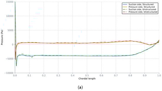
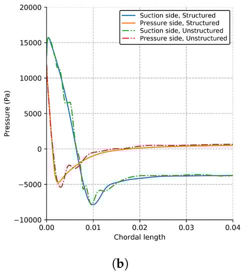
Figure 9.
Pressure distribution along the blade (a) and around the leading edge (b) for radial section at m.
Unstructured grids with refinements in key regions achieve much better results while still respecting the imposed cell limit for a single passage. For the lowest advance ratio, trust and torque coefficient predictions are within when compared to the experiment, while for the remaining range errors are below (Figure 10). However, our previous observation still stands; despite better overall results, blade profile representation is still lacking and pressure oscillations are common. Numerical results obtained on unstructured grids should therefore be considered with caution and their validity corroborated with additional data on geometry and pressure distribution. For initial performance projections, unstructured grids might be beneficial, but should not be a definitive CFD solution to performance analysis of a propeller. Nonetheless, these results are still respectable and in relative accordance with the results attained using structured grids. The summary of results for unstructured grids is given in Table A1.
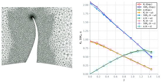
Figure 10.
Refined unstructured grid (left) and open water results for refined unstructured grid using SST k- and Realizable k- model (right).
Contrary to the results obtained for unstructured grids, switching from SST k- to Realizable model when using structured grids has led to improvements in both thrust and torque coefficient predictions. Discrepancy between Fluent CFD results and experimental measurements is , even at highest advance ratios. STAR-CCM+ shows improvements when compared to k- model up to for low and high ratios. Comparison with the experimental results can be seen in Figure 11. It is important to note that Realizable k- model struggles with convergence at higher advance ratios and therefore requires longer computational time to reach steady results. Furthermore, for , SST k- models is significantly more stable with much quicker convergence.
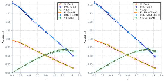
Figure 11.
Calculated open water characteristics for structured grids and Realizable k- model in: Fluent (left); STAR-CCM+ (right).
Thrust and torque coefficients obtained using Realizable k- model, on average, correlate better to the experimental data, when compared to SST k- model. At the same time, despite better coherence, calculated efficiency results when evaluating advance ratios near the operating point diverge more than values obtained with the SST k-. These results are an inherent consequence of the equations governing the relation between coefficients; if errors for both thrust and torque increase in the same manner, resulting efficiency will remain unchanged. It is evident that Realizable model provides better thrust predictions, especially for . Torque values are mostly overestimated in Fluent with errors up to and underestimated in STAR-CCM+. Relative errors for discussed two-equation turbulent models are given in Figure 12. An overview of numerically attained values for hydrodynamic coefficients in both solvers is given in Table A2 and Table A3.
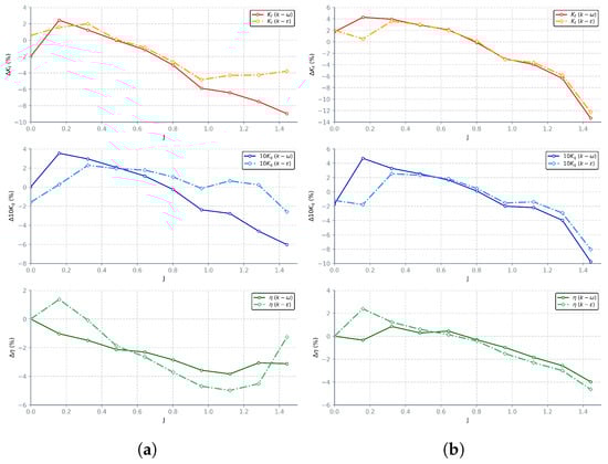
Figure 12.
Relative errors in hydrodynamic coefficient predictions for structured grids attained with SST k- and Realizable k- models in: Fluent (a); STAR-CCM+ (b).
3.2. Cavitation Test
Cavitating flow simulation was done for adjusted advance ratio and s. This correction minimizes the discrepancy between experimental measurements and analyzed “realistic” open water condition. The calculated cavitating flow potential for conducted tests is . Zwart–Gerber–Belamri (ZGB) and Schnerr and Sauer models were employed, both one-equation models which employ a no-slip condition between liquid and vapor phases. The ZGB model is based on Rayleigh–Plesset equation with bubble radius and nucleation site volume fraction as parameters [30,31]. The Sauer model, aside from bubble radius, requires bubbles count per volume to be estimated [30,31]. Transient analysis with an approximate run time of s corresponding to 10 revolutions was conducted, using steady state results as an initial estimation. Courant number was maintained below 2 for the first five revolutions and below 0.5 for the remaining evaluation time with variable time stepping. For every time step, a maximum of 20 iterations was allowed with convergence set at . Thrust and torque were calculated as an average of the values in the final revolution. Analogously to open water calculations, attained numerical results were used to calculate thehydrodynamic characteristics shown in Table 1.

Table 1.
Hydrodynamic characteristics of a cavitating propeller for calculated using STAR-CCM+ and Fluent.
Efficiency, thrust and torque coefficients when using Sauer model show good agreement with the experimental data. STAR-CCM+ provides marginally better results than Fluent. In both cases, relative differences are below . These results are comparable to values attained using more sophisticated methods [5,18]. Adoption of the ZBR model offered no significant improvements. Predicted cavitation patterns using structured grids for vapor volume fraction are shown in Figure 13. Similarly sized unstructured grids could not achieve prescribed residual convergence during the final revolution, thus they have been deemed inadequate.
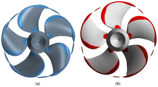
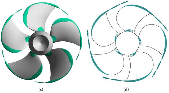
Figure 13.
Cavity extents for vapor volume fraction: STAR-CCM+ with Schnerr and Sauer model (a); Fluent with Schnerr and Sauer model (b); Fluent with Zwart–Gerber–Belamri model (c); experimental observations (d).
Cavity extents on suction side for both solvers and models are similar; however, when compared to the experimental data (Figure 13d), the difference is noticeable. Tip vortex cavitation is reasonably well predicted, with minor inaccuracies. Breakdown of the vortex rope can be attributed to the missing refinement region behind the blade. Sheet cavitation near the propeller hub is mostly in accordance with the experiment. Overestimation of the sheet cavitation near the leading edge is the most erroneous. One potential cause is grid deficiency. Implemented cavitation models could also be inadequate for desired level of accuracy. The definitive reason for the disagreement with the experiment requires further investigation. Cavitation analysis for the entire range of advance ratios will be conducted in upcoming works.
4. Conclusions
Current RANS based approaches for marine propeller performance analyses were thoroughly investigated in this study. Different turbulent models and solvers using hexahedral block structured grids and hybrid unstructured grids were assessed and corresponding predictions compared to the experimental data. Results were attained for open water and cavitation tunnel tests. Grid sensitivity study was performed to determine appropriate grids for all tests. Hydrodynamic characteristics for open water tests were evaluated throughout the full range of advance ratios. Cavitation tests were conducted for selected advance ratio and two distinct cavitation models.
Open water results are in very good agreement with the experimental data across all tests, with errors below on average and at worst up to for structured grids and Realizable k- model. Tetrahedral unstructured grid’s prediction errors are within for the lowest advance ratios and on average; unfortunately, pertinence of these results is questionable. Key findings are as follows:
- Different RANS solvers behave similarly with marginal deviations.
- Structured and unstructured grids can achieve comparable levels of accuracy. Therefore, depending on the requirements, unstructured tetrahedral grids can be an acceptable choice considering they are much simpler to generate. When employing tetrahedral grids, it is important to determine whether the results are a consequence of cumulative numerical errors and incomplete geometric representation. Imposed limitations on grid size can lead to inadequacies, which might be annulled by numerical errors. Deficiencies of tetrahedral grids could be mitigated by employing hexa-dominant or polyhedral unstructured grids. If accuracy of the results is in primary focus, structured grids should be preferred.
- Grid sensitivity study revealed steady convergence in prediction accuracy with the increase in grid size. The results obtained with coarse grids emphasize the importance of grid density and refinements. Therefore, to achieve relatively accurate results while maintaining representability, a minimum of cells per blade should be used to properly depict a propeller.
- SST k- and Realizable k- models provide similar results; however, the Realizable model seems to provide both consistent and more accurate results, especially at higher advance ratios. SST k- could be beneficial for lower advance ratios and wall-bounded flows.
- Variances in performance predictions can be partially attributed to unresolved transition from laminar flow regime to turbulent flow along the propeller walls. Increase in Reynolds number usually leads to discernible variations of hydrodynamic characteristics at higher advance ratios, which was clearly demonstrated. Influence of Reynolds number is not incorporated in current results and cannot be properly resolved using common two-equation RANS models.
- Propeller performance predictions in cavitating conditions are also satisfactory, with errors below for analyzed case when using both Schnerr and Sauer and Zwart–Gerber–Belamri models. Cavitation models showed no significant differences in prediction accuracy. Tip vortex cavitation shape and extent predictions can be improved with grid refinement near the tip and in regions behind the blade, where cavitation rope is expected. Additionally, full model simulations could provide better results. Sheet cavitation needs to be further investigated, especially near the leading edge where cavitation pattern deviates the most. Employed coarse grids undoubtedly have an impact on cavity extents and thus grids should be refined appropriately in further studies.
Advantages of the hexahedral block structured grids for open water and cavitation analyses have been clearly demonstrated. Difficulties in grid generation are outweighed by several benefits; structured grids are robust, which can be clearly seen in cavitation tests, they are better at capturing geometric features while using fewer cells and are simpler to numerically solve, which can lead to significant reductions in overall computational time. Therefore, they should be considered as a centerpiece of marine propeller analyses and used in conjunction with Realizable k- model, which exhibits good overall accuracy and stability across all test cases.
Author Contributions
A.S. designed CFD models for all test cases and conducted analysis in Fluent. Z.Č. conducted analysis in STAR-CCM+. Most of the paper was written by A.S. with contributions and revisions by I.L. under the supervision of Z.Č. L.K. provided theoretical support and guidance with regards to methodology as well as conducted key revisions.
Funding
This research received no external funding.
Conflicts of Interest
The authors declare no conflict of interest.
Abbreviations
The following abbreviations are used in this manuscript:
| CFD | Computational Fluid Dynamics |
| PPTC | Postdam Propeller Test Case |
| BET | Blade Element Theory |
| BEMT | Blade Element Momentum Theory |
| IBLM | Integral Boundary Layer Method |
| BEM | Boundary Element Method |
| DNS | Direct Numerical Simulations |
| LES | Large Eddy Simulations |
| RANS | Reynolds-averaged Navier–Stokes |
| SST | Shear Stress Transport |
| RSM | Reynolds Stress Model |
| TSM | Transition Sensitive Turbulence Model |
| DDES | Delayed Detached Eddy Simulation |
| SIMPLE | Semi-implicit Method For Pressure Linked Equations |
| HRIC | High Resolution Interface Capturing |
| SRF | Single Moving Reference Frame |
| ZGB | Zwart–Gerber–Belamri |
Appendix A
Table A1.
Open water hydrodynamic characteristics for unstructured grids.
Table A1.
Open water hydrodynamic characteristics for unstructured grids.
| Unstructured | ||||||||||||
|---|---|---|---|---|---|---|---|---|---|---|---|---|
| Realizable - | SST - | Realizable -, Fine | SST -, Fine | |||||||||
| 0.000 | 0.468 | 1.069 | 0.000 | 0.587 | 1.252 | 0.000 | 0.954 | 2.063 | 0.000 | 0.937 | 2.046 | 0.000 |
| 0.160 | 0.476 | 1.139 | 0.106 | 0.540 | 1.163 | 0.118 | 0.915 | 1.936 | 0.120 | 0.869 | 1.883 | 0.118 |
| 0.322 | 0.846 | 1.783 | 0.243 | 0.844 | 1.772 | 0.244 | 0.821 | 1.753 | 0.240 | 0.791 | 1.712 | 0.237 |
| 0.482 | 0.754 | 1.620 | 0.357 | 0.750 | 1.608 | 0.357 | 0.716 | 1.568 | 0.350 | 0.696 | 1.536 | 0.347 |
| 0.642 | 0.653 | 1.446 | 0.462 | 0.654 | 1.439 | 0.464 | 0.609 | 1.380 | 0.451 | 0.602 | 1.372 | 0.448 |
| 0.802 | 0.553 | 1.277 | 0.553 | 0.554 | 1.268 | 0.558 | 0.504 | 1.198 | 0.537 | 0.507 | 1.208 | 0.535 |
| 0.961 | 0.455 | 1.105 | 0.629 | 0.454 | 1.093 | 0.636 | 0.406 | 1.026 | 0.605 | 0.412 | 1.037 | 0.607 |
| 1.121 | 0.358 | 0.927 | 0.688 | 0.357 | 0.912 | 0.698 | 0.313 | 0.856 | 0.652 | 0.321 | 0.860 | 0.665 |
| 1.283 | 0.261 | 0.733 | 0.726 | 0.260 | 0.720 | 0.737 | 0.219 | 0.671 | 0.667 | 0.230 | 0.673 | 0.699 |
| 1.442 | 0.162 | 0.524 | 0.707 | 0.162 | 0.517 | 0.720 | 0.124 | 0.470 | 0.608 | 0.140 | 0.504 | 0.639 |
Table A2.
Open water hydrodynamic characteristics for structured grid obtained with Fluent.
Table A2.
Open water hydrodynamic characteristics for structured grid obtained with Fluent.
| Structured, Fluent | ||||||
|---|---|---|---|---|---|---|
| Realizable - | SST - | |||||
| 0.000 | 0.960 | 2.047 | 0.000 | 0.936 | 2.080 | 0.000 |
| 0.160 | 0.907 | 1.947 | 0.119 | 0.915 | 2.010 | 0.116 |
| 0.322 | 0.815 | 1.777 | 0.235 | 0.808 | 1.788 | 0.232 |
| 0.482 | 0.702 | 1.576 | 0.342 | 0.701 | 1.578 | 0.341 |
| 0.642 | 0.598 | 1.391 | 0.439 | 0.596 | 1.383 | 0.441 |
| 0.802 | 0.496 | 1.212 | 0.523 | 0.494 | 1.196 | 0.527 |
| 0.961 | 0.400 | 1.038 | 0.589 | 0.396 | 1.015 | 0.596 |
| 1.121 | 0.310 | 0.866 | 0.638 | 0.303 | 0.837 | 0.646 |
| 1.283 | 0.222 | 0.685 | 0.662 | 0.214 | 0.652 | 0.672 |
| 1.442 | 0.135 | 0.490 | 0.633 | 0.128 | 0.473 | 0.621 |
Table A3.
Open water hydrodynamic characteristics for structured grid obtained with STAR-CCM+.
Table A3.
Open water hydrodynamic characteristics for structured grid obtained with STAR-CCM+.
| Structured, STAR-CCM+ | ||||||
|---|---|---|---|---|---|---|
| Realizable - | SST - | |||||
| 0.000 | 0.974 | 2.055 | 0.000 | 0.971 | 2.045 | 0.000 |
| 0.160 | 0.897 | 1.907 | 0.120 | 0.931 | 2.032 | 0.117 |
| 0.322 | 0.827 | 1.781 | 0.238 | 0.830 | 1.794 | 0.237 |
| 0.482 | 0.723 | 1.582 | 0.350 | 0.722 | 1.585 | 0.349 |
| 0.642 | 0.615 | 1.392 | 0.452 | 0.616 | 1.389 | 0.453 |
| 0.802 | 0.510 | 1.205 | 0.541 | 0.509 | 1.201 | 0.541 |
| 0.961 | 0.407 | 1.024 | 0.609 | 0.408 | 1.019 | 0.612 |
| 1.121 | 0.312 | 0.849 | 0.656 | 0.311 | 0.842 | 0.660 |
| 1.283 | 0.218 | 0.663 | 0.672 | 0.217 | 0.656 | 0.675 |
| 1.442 | 0.123 | 0.463 | 0.611 | 0.122 | 0.454 | 0.615 |
References
- Yeo, K.B.; Hau, W.Y. Fundamentals of Marine Propeller Analysis. J. Appl. Sci. 2014, 14, 1078–1082. [Google Scholar] [CrossRef]
- Gur, O.; Rosen, A. Comparison between blade-element models of propellers. Aeronaut. J. 2008, 112, 689–704. [Google Scholar] [CrossRef]
- Benini, E. Significance of blade element theory in performance prediction of marine propellers. Ocean Eng. 2004, 31, 957–974. [Google Scholar] [CrossRef]
- Gaggero, S.; Villa, D. Steady cavitating propeller performance by using OpenFOAM, StarCCM+ and a boundary element method. Proc. Inst. Mech. Eng. Part M J. Eng. Marit. Environ. 2017, 231, 411–440. [Google Scholar] [CrossRef]
- Vaz, G.; Hally, D.; Huuva, T.; Bulten, N.; Muller, P.; Becchi, P.; Herrer, J.L.; Whitworth, S.; Macé, R.; Korsström, A. Cavitating flow calculations for the E779A propeller in open water and behind conditions: Code comparison and solution validation. In Proceedings of the 4th International Symposium on Marine Propulsors (SMP ’15), Austin, TX, USA, 31 May–4 June 2015; pp. 330–345. [Google Scholar]
- Rijpkema, D.; Vaz, G. Viscous flow computations on propulsors: Verification, validation and scale effects. In Proceedings of the Developments in Marine CFD, London, UK, 22–23 March 2011. [Google Scholar]
- Bensow, R.E.; Bark, G. Implicit LES predictions of the cavitating flow on a propeller. J. Fluids Eng. 2010, 132, 041302. [Google Scholar] [CrossRef]
- Baltazar, J.; Falcão de Campos, J.; Bosschers, J. Open-water thrust and torque predictions of a ducted propeller system with a panel method. Int. J. Rotating Mach. 2012, 2012. [Google Scholar] [CrossRef]
- Baltazar, J.; Rijpkema, D.; Falcão de Campos, J.; Bosschers, J. Prediction of the open-water performance of ducted propellers with a panel method. J. Mar. Sci. Eng. 2018, 6, 27. [Google Scholar] [CrossRef]
- Pereira, F.; Salvatore, F.; Di Felice, F. Measurement and modeling of propeller cavitation in uniform inflow. J. Fluids Eng. 2004, 126, 671–679. [Google Scholar] [CrossRef]
- Bosschers, J.; Vaz, G.; Starke, A.; van Wijngaarden, E. Computational analysis of propeller sheet cavitation and propeller-ship interaction. In Proceedings of the RINA Conference MARINE CFD2008, Southampton, UK, 26–27 March 2008; pp. 26–27. [Google Scholar]
- Bosschers, J.; Willemsen, C.; Peddle, A.; Rijpkema, D. Analysis of ducted propellers by combining potential flow and RANS methods. In Proceedings of the Fourth International Symposium on Marine Propulsors, Austin, TX, USA, 31 May–4 June 2015; pp. 639–648. [Google Scholar]
- Bhattacharyya, A.; Krasilnikov, V.; Steen, S. A CFD-based scaling approach for ducted propellers. Ocean Eng. 2016, 123, 116–130. [Google Scholar] [CrossRef]
- Krasilnikov, V.; Sun, J.; Halse, K.H. CFD investigation in scale effect on propellers with different magnitude of skew in turbulent flow. In Proceedings of the First International Symposium on Marine Propulsors, Trondheim, Norway, 22–24 June 2009; pp. 25–40. [Google Scholar]
- Morgut, M.; Nobile, E. Influence of grid type and turbulence model on the numerical prediction of the flow around marine propellers working in uniform inflow. Ocean Eng. 2012, 42, 26–34. [Google Scholar] [CrossRef]
- Wang, X.; Walters, K. Computational analysis of marine-propeller performance using transition-sensitive turbulence modeling. J. Fluids Eng. 2012, 134, 071107. [Google Scholar] [CrossRef]
- Helal, M.M.; Ahmed, T.M.; Banawan, A.A.; Kotb, M.A. Numerical prediction of sheet cavitation on marine propellers using CFD simulation with transition-sensitive turbulence model. Alex. Eng. J. 2018, 57, 3805–3815. [Google Scholar] [CrossRef]
- Viitanen, V.; Hynninen, A.; Sipilä, T.; Siikonen, T. DDES of wetted and cavitating marine propeller for CHA underwater noise assessment. J. Mar. Sci. Eng. 2018, 6, 56. [Google Scholar] [CrossRef]
- Tu, T.N. Numerical simulation of propeller open water characteristics using RANSE method. Alex. Eng. J. 2019, 58, 531–537. [Google Scholar] [CrossRef]
- Da-Qing, L. Validation of RANS predictions of open water performance of a highly skewed propeller with experiments. J. Hydrodyn. Ser. B 2006, 18, 520–528. [Google Scholar]
- Rhee, S.H.; Joshi, S. CFD validation for a marine propeller using an unstructured mesh based RANS method. In Proceedings of the ASME/JSME 2003 4th Joint Fluids Summer Engineering Conference, Honolulu, HI, USA, 6–10 July 2003; American Society of Mechanical Engineers: New York, NY, USA, 2003; pp. 1157–1163. [Google Scholar]
- SVA Team. PPTC SMP’11 Workshop. 2011. Available online: https://www.sva-potsdam.de/pptc-smp11-workshop/ (accessed on 7 May 2019).
- Subhas, S.; Saji, V.; Ramakrishna, S.; Das, H. CFD analysis of a propeller flow and cavitation. Int. J. Comput. Appl. 2012, 55, 26–33. [Google Scholar]
- Ferziger, J.H.; Peric, M. Computational Methods for Fluid Dynamics; Springer Science & Business Media: Berlin/Heidelberg, Germany, 2012. [Google Scholar]
- Djahida, B.; Omar, I. Numerical simulation of the cavitating flow around marine co-rotating tandem propellers. Brodogr. Teor. Praksa Brodogr. Pomor. Teh. 2019, 70, 43–57. [Google Scholar] [CrossRef]
- Papakonstantinou, T.; Grigoropoulos, G.; Papadakis, G. Marine Propeller Optimization using Open-Source CFD. In Sustainable Development and Innovations in Marine Technologies, Proceedings of the 18th International Congress of the Maritme Association of the Mediterranean (IMAM 2019), Varna, Bulgaria, 9–11 September 2019; CRC Press: Boca Raton, FL, USA, 2019; p. 252. [Google Scholar]
- Guilmineau, E.; Deng, G.; Leroyer, A.; Queutey, P.; Visonneau, M.; Wackers, J. Numerical simulations of the cavitating and non-cavitating flow around the postdam propeller test case. In Proceedings of the Fourth International Symposium on Marine Propulsors (SMP ’15), Austin, TX, USA, 31 May–4 June 2015; Volume 15. [Google Scholar]
- Wang, W.; Zhao, D.; Guo, C.; Pang, Y. Analysis of Hydrodynamic Performance of L-Type Podded Propulsion with Oblique Flow Angle. J. Mar. Sci. Eng. 2019, 7, 51. [Google Scholar] [CrossRef]
- Owen, D.; Demirel, Y.K.; Oguz, E.; Tezdogan, T.; Incecik, A. Investigating the effect of biofouling on propeller characteristics using CFD. Ocean Eng. 2018, 159, 505–516. [Google Scholar] [CrossRef]
- Kozubková, M.; Rautová, J.; Bojko, M. Mathematical model of cavitation and modelling of fluid flow in cone. Procedia Eng. 2012, 39, 9–18. [Google Scholar] [CrossRef]
- Chiang, S.; Chen, J. A comparison study of different cavitation models on the development of 2-D cavitating flows. In Proceedings of the 12th International Conference on Hydrodynamics, Egmond aan Zee, The Netherlands, 18–23 September 2016; pp. 18–23. [Google Scholar]
© 2019 by the authors. Licensee MDPI, Basel, Switzerland. This article is an open access article distributed under the terms and conditions of the Creative Commons Attribution (CC BY) license (http://creativecommons.org/licenses/by/4.0/).