Stability Assessment of Rubble Mound Breakwaters Using Extreme Learning Machine Models

 ,
,
Abstract
1. Introduction
2. Extreme Learning Machine Models
2.1. Fundamental of Extreme Learning Machine Model
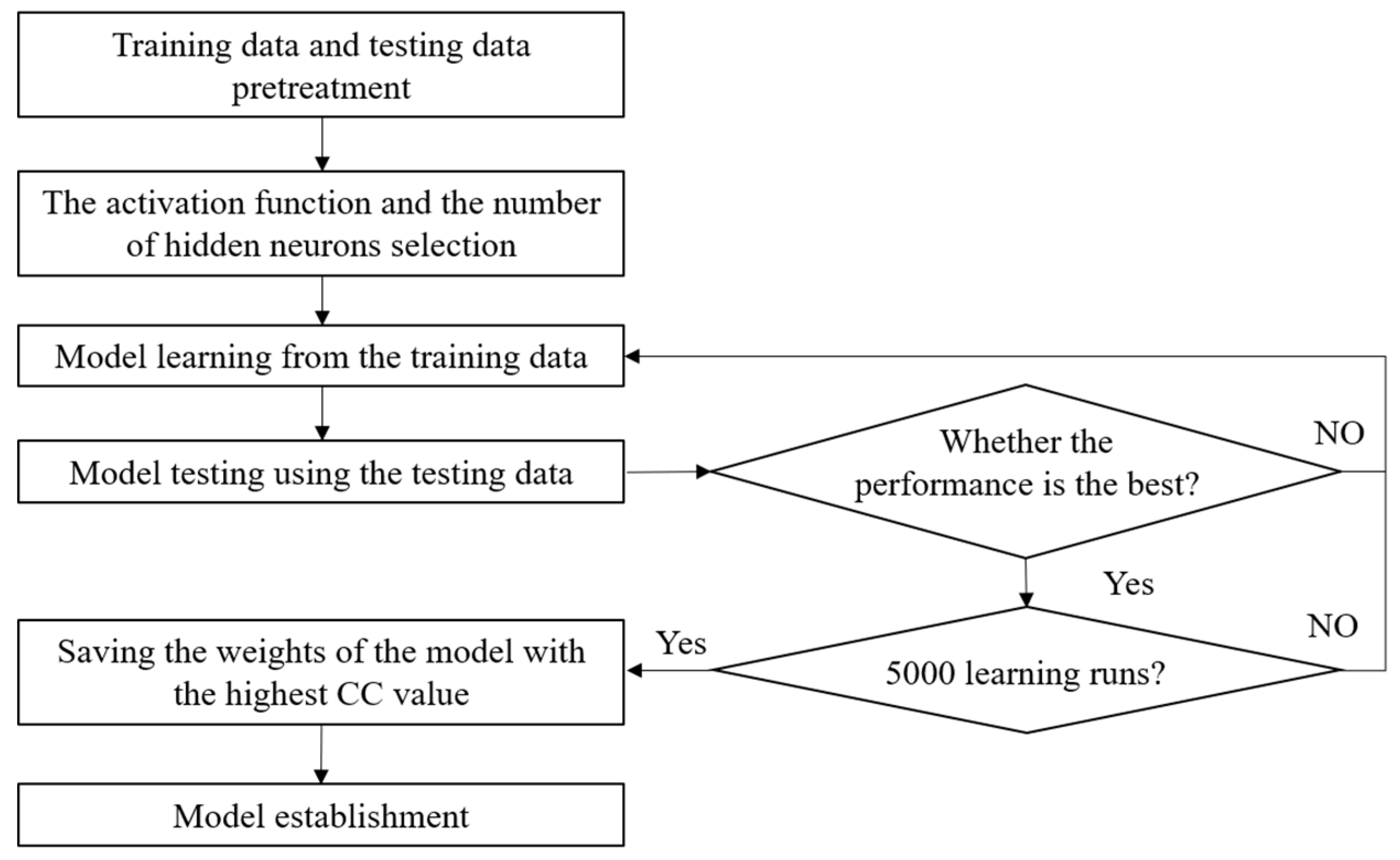
2.2. Model Establishment
3. Results and Discussion
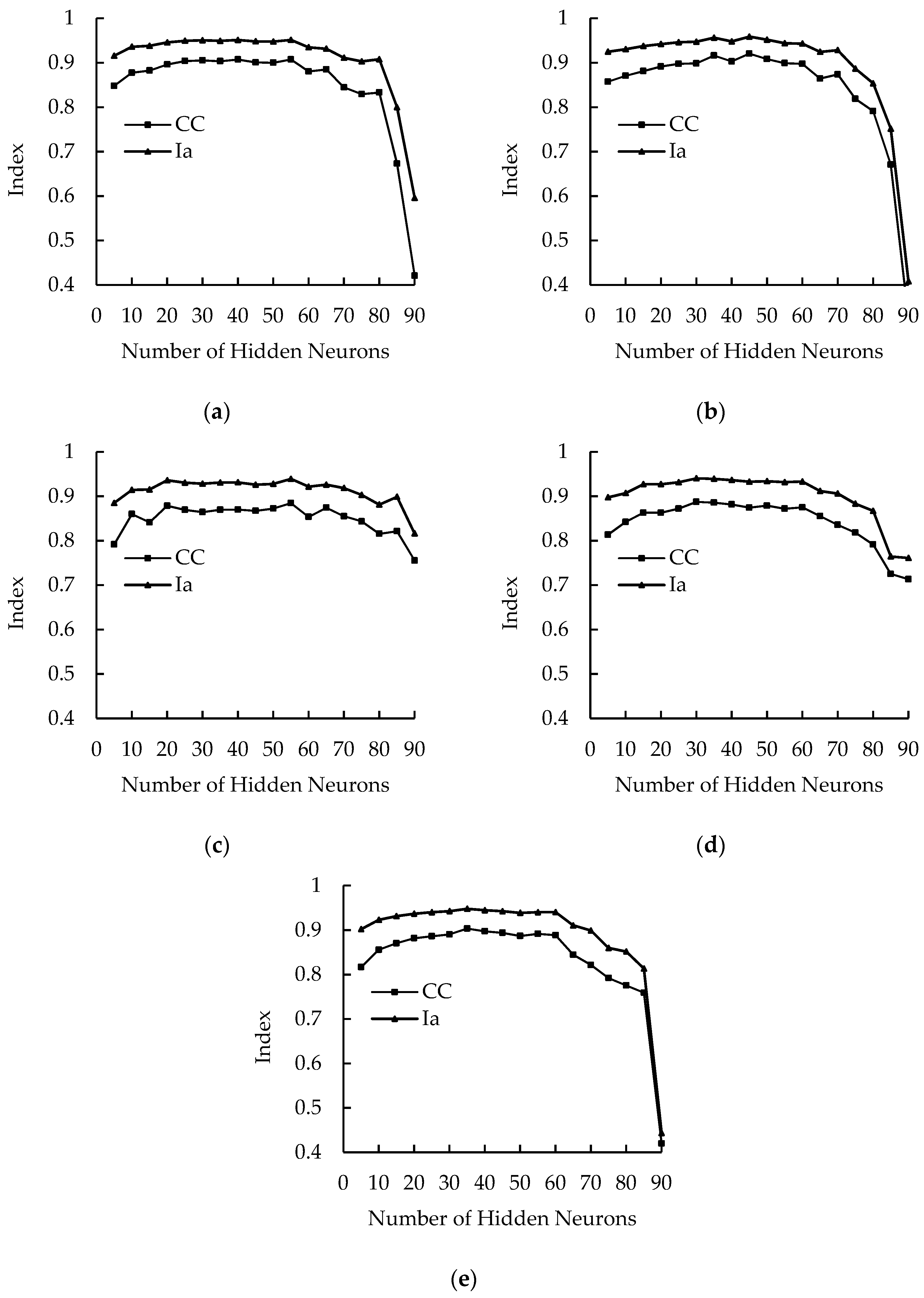
3.1. The Influence of Hidden Neurons on the Assessment Performance of ELM Models with Different Activation Functions
3.2. Predicted Performance Comparison of Different Methods
4. Conclusions
Supplementary Materials
Author Contributions
Funding
Acknowledgments
Conflicts of Interest
Appendix A

| 0.5241 | 26.4975 | 0.8109 | −0.4255 | 0.6935 | −0.2008 | |||
| 0.5979 | −3.6891 | 0.8853 | 0.6774 | 0.6278 | −0.9448 | |||
| 0.6609 | 4.1169 | 0.1518 | 0.2682 | 0.2991 | 0.0216 | |||
| 0.9402 | 1.1036 | −0.5524 | 0.7574 | 0.7449 | −0.6862 | |||
| 0.1974 | −32.1789 | −0.3415 | 0.2084 | −0.7634 | −0.1137 | |||
| 0.8710 | −3.2400 | −0.6313 | 0.8539 | −0.3247 | 0.9143 | |||
| 0.7430 | −29.8057 | 0.3799 | −0.2154 | −0.7326 | −0.9678 | |||
| 0.2418 | 5.5068 | −0.8844 | 0.7903 | 0.7482 | −0.7737 | |||
| 0.5977 | −22.8297 | 0.1486 | −0.9762 | 0.4362 | 0.0493 | |||
| 0.7125 | 1.7637 | 0.1595 | 0.5090 | −0.9902 | 0.1901 | |||
| 0.1448 | 21.5258 | −0.5829 | 0.0194 | −0.7497 | −0.6622 | |||
| 0.4441 | −4.4733 | −0.8343 | 0.7352 | 0.8387 | −0.2093 | |||
| 0.1918 | 6.0145 | −0.7073 | 0.0374 | 0.8523 | 0.7221 | |||
| 0.7374 | 52.4679 | −0.4033 | −0.0100 | 0.8501 | −0.7359 | |||
| 0.1496 | −9.1100 | 0.6958 | −0.2846 | 0.9258 | −0.7403 | |||
| 0.1726 | −3.6265 | 0.4105 | −0.9711 | 0.5676 | −0.2996 | |||
| 0.8718 | −8.6176 | −0.9463 | −0.0608 | −0.5387 | −0.6198 | |||
| 0.8638 | 32.5670 | 0.7170 | 0.0887 | −0.4715 | −0.5685 | |||
| 0.2632 | 13.7757 | 0.1976 | −0.0730 | −0.7203 | −0.0630 | |||
| 0.1091 | −9.6165 | 0.0072 | −0.6522 | 0.2843 | 0.5996 | |||
| 0.3324 | 3.5370 | 0.3308 | 0.2424 | −0.6404 | 0.6969 | |||
| BHN1= | 0.1969 | InW1= | −30.1128 | InW2= | −0.7382 | −0.5162 | −0.7029 | 0.4078 |
| 0.5033 | 40.9492 | −0.1724 | −0.1571 | 0.2812 | −0.6081 | |||
| 0.7217 | −2.1417 | 0.0027 | −0.1367 | 0.9792 | −0.1936 | |||
| 0.0935 | −4.5602 | 0.7380 | −0.4168 | 0.7734 | −0.7967 | |||
| 0.8949 | −7.4840 | −0.8876 | −0.7521 | 0.7573 | 0.1826 | |||
| 0.9296 | −51.8195 | −0.3970 | 0.0788 | 0.6631 | −0.9412 | |||
| 0.3114 | −32.1941 | 0.5991 | 0.3968 | −0.0596 | 0.2747 | |||
| 0.8365 | 0.7267 | 0.9239 | 0.6791 | 0.7207 | −0.1689 | |||
| 0.6055 | 35.3792 | −0.4155 | −0.4794 | −0.8263 | −0.0045 | |||
| 0.1465 | 5.8143 | −0.9828 | −0.4143 | 0.2699 | 0.9241 | |||
| 0.9326 | −14.1016 | 0.5911 | 0.8271 | 0.5772 | 0.0635 | |||
| 0.1928 | 9.7569 | −0.4223 | −0.3700 | 0.2338 | 0.7443 | |||
| 0.4138 | 2.4507 | −0.1683 | −0.2665 | −0.5608 | 0.6952 | |||
| 0.0855 | −7.5543 | −0.9139 | −0.9217 | −0.7361 | −0.3699 | |||
| 0.7125 | 8.2359 | −0.7147 | 0.3655 | −0.7379 | −0.7774 | |||
| 0.5891 | 3.9906 | 0.4442 | 0.7030 | 0.2163 | 0.0113 | |||
| 0.8273 | 1.0311 | 0.9852 | 0.9763 | −0.4108 | −0.4178 | |||
| 0.4677 | 11.6137 | −0.2928 | −0.8980 | −0.1545 | 0.3437 | |||
| 0.6765 | 6.5585 | 0.2751 | 0.9346 | 0.7867 | 0.6949 | |||
| 0.3229 | −7.2543 | −0.1302 | 0.1766 | 0.9851 | −0.9479 | |||
| 0.7244 | −8.8476 | −0.4926 | 0.8206 | 0.0350 | −0.9965 | |||
| 0.1206 | −10.8684 | 0.0382 | −0.5207 | 0.0727 | 0.9225 | |||
| 0.5268 | −5.1499 | −0.1425 | −0.2191 | 0.4494 | −0.9388 | |||
| 0.2891 | 8.4672 | 0.6724 | 0.1706 | −0.4620 | 0.9983 |
| 0.4319 | −42.0761 | −0.9071 | −0.2011 | 0.4272 | 0.8116 | |||
| 0.0320 | −20.9949 | −0.3291 | −0.0591 | −0.4020 | 0.8705 | |||
| 0.5944 | −32.7021 | −0.8404 | −0.6064 | 0.8841 | 0.6630 | |||
| 0.6627 | 43.8901 | −0.7591 | −0.2472 | 0.8186 | 0.9823 | |||
| 0.9264 | 13.2387 | 0.8394 | −0.8762 | −0.1618 | −0.3568 | |||
| 0.5949 | −20.2892 | 0.5871 | 0.8688 | −0.0913 | 0.7016 | |||
| 0.8525 | −63.1985 | 0.3422 | −0.7897 | −0.4640 | −0.2132 | |||
| 0.8806 | −116.6938 | 0.2035 | −0.5851 | −0.2849 | −0.8588 | |||
| 0.6270 | −13.5202 | 0.7838 | 0.9148 | −0.8121 | 0.6147 | |||
| 0.2328 | 35.2013 | −0.1258 | −0.3481 | −0.7869 | −0.1297 | |||
| 0.2941 | 3.1475 | −0.8012 | 0.0277 | −0.4674 | −0.6218 | |||
| 0.2577 | 12.4026 | −0.8559 | −0.6591 | −0.9608 | 0.2650 | |||
| 0.6162 | 0.2601 | −0.4507 | −0.2077 | −0.4970 | 0.7523 | |||
| 0.1584 | −3.0225 | 0.9716 | 0.8243 | −0.4446 | 0.6805 | |||
| 0.5654 | −7.7516 | −0.6291 | −0.5789 | −0.5272 | 0.3921 | |||
| 0.5730 | 5.6515 | −0.2855 | −0.5305 | 0.4384 | 0.8396 | |||
| 0.6728 | 27.5190 | 0.0217 | 0.4931 | −0.1090 | −0.5729 | |||
| 0.7424 | 0.7453 | −0.4198 | 0.1380 | 0.4327 | −0.9063 | |||
| 0.7593 | 36.1610 | 0.4848 | 0.2726 | 0.6648 | 0.6994 | |||
| 0.7122 | 44.1426 | −0.6639 | −0.4197 | 0.5753 | 0.2885 | |||
| 0.6100 | −16.2722 | −0.0565 | −0.0394 | 0.8366 | −0.8595 | |||
| BHN2= | 0.0537 | InW2= | −1.1557 | InW2= | −0.7270 | −0.1948 | −0.1188 | −0.1234 |
| 0.4458 | 22.3288 | 0.5387 | 0.8696 | −0.4597 | 0.9628 | |||
| 0.8475 | −1.6268 | 0.7513 | −0.9025 | −0.6607 | 0.6460 | |||
| 0.9733 | −83.7627 | 0.3622 | −0.6518 | −0.4596 | −0.5125 | |||
| 0.8544 | 22.4302 | 0.8799 | −0.2234 | −0.4083 | −0.7212 | |||
| 0.3858 | −21.6072 | −0.5399 | 0.1999 | 0.1068 | −0.4392 | |||
| 0.9096 | −2.8837 | −0.4029 | −0.6285 | 0.8447 | −0.2820 | |||
| 0.1069 | −28.1949 | −0.7637 | 0.7851 | −0.3326 | −0.1881 | |||
| 0.2582 | −18.8255 | −0.0014 | −0.1194 | 0.5881 | 0.2810 | |||
| 0.5765 | 47.8772 | 0.5480 | −0.4075 | −0.7139 | −0.6196 | |||
| 0.3990 | −5.0568 | 0.8476 | 0.1595 | −0.4691 | 0.1434 | |||
| 0.3779 | 9.6864 | 0.7929 | −0.4492 | −0.8683 | −0.4401 | |||
| 0.3411 | 10.6359 | −0.4233 | 0.5854 | −0.9226 | 0.3489 | |||
| 0.2897 | 3.4956 | 0.8980 | −0.7244 | 0.0454 | 0.2533 | |||
| 0.7287 | 45.6903 | −0.4528 | 0.5858 | 0.1254 | −0.0241 | |||
| 0.7738 | −45.6212 | 0.8116 | −0.2095 | −0.0985 | −0.6733 | |||
| 0.5252 | 25.9720 | 0.2493 | −0.7998 | −0.2112 | −0.3585 | |||
| 0.8545 | −50.5003 | −0.0441 | 0.5296 | −0.0523 | 0.2865 | |||
| 0.0416 | 3.4476 | −0.8948 | 0.9645 | −0.8378 | 0.9041 | |||
| 0.6695 | 8.8539 | −0.6859 | −0.9783 | −0.8757 | −0.9541 | |||
| 0.8819 | 20.7560 | 0.0010 | 0.8347 | −0.0483 | −0.2737 | |||
| 0.9352 | 133.8480 | 0.2844 | −0.8046 | −0.2266 | −0.8481 | |||
| 0.1300 | 5.0666 | 0.6626 | −0.6074 | 0.4537 | −0.5816 | |||
| 0.9134 | 14.3699 | −0.5942 | 0.5127 | −0.0012 | −0.3285 |
Appendix B
References
- Hudson, Y. Laboratory investigation of rubble-mound breakwater. Proc. ASCE 1959, 85, 93–122. [Google Scholar]
- Van der Meer, J.W. Rock Slopes and Gravel Beaches under Wave Attack; Delft University of Technology: Delft, The Netherlands, 1988. [Google Scholar]
- Pilarczyk, K. Dikes and Revetments Design, Maintenance and Safety Assessment; Routledge: London, UK, 1998. [Google Scholar]
- Meulen, T.v.d.; Schiereck, G.J.; d’Angremond, K. Rock toe stability of rubble mound breakwaters. Coast. Eng. 1996, 83, 1971–1984. [Google Scholar]
- Kajima, R. A new method of structurally resistive design of very important seawalls against wave action. In Proceedings of the Wave Barriers in Deepwaters, Yokosuka, Japan, 10–14 January 1994; pp. 518–536. [Google Scholar]
- Hanzawa, M.; Sato, H.; Takahashi, S.; Shimosako, K.; Takayama, T.; Tanimoto, K. Chapter 130 New Stability Formula for Wave-Dissipating Concrete Blocks Covering Horizontally Composite Breakwaters. In Proceedings of the Coastal Engineering 1996, Orlando, FL, USA, 2–6 September 1996. [Google Scholar]
- Vidal, C.; Medina, R.; Lomónaco, P. Wave height parameter for damage description of rubble-mound breakwaters. Coast. Eng. 2006, 53, 711–722. [Google Scholar] [CrossRef]
- Etemad-Shahidi, A.; Bonakdar, L. Design of rubble-mound breakwaters using M5′ machine learning method. Appl. Ocean Res. 2009, 31, 197–201. [Google Scholar] [CrossRef]
- Van Gent, M.R.A.; Der Werf, I.V. Rock toe stability of rubble mound breakwaters. Coast. Eng. 2014, 83, 166–176. [Google Scholar] [CrossRef]
- Thompson, D.M.; Shuttler, R.M. Riprap Design for Wind-Wave Attack, a Laboratory Study in Random Waves; HR Wallingford: Wallingford, UK, 1975. [Google Scholar]
- Wei, X.; Lu, Y.; Wang, Z.; Liu, X.; Mo, S. A Machine Learning Approach to Evaluating the Damage Level of Tooth-Shape Spur Dikes. Water 2018, 10, 1680. [Google Scholar] [CrossRef]
- Dong, H.K.; Park, W.S. Neural network for design and reliability analysis of rubble mound breakwaters. Ocean Eng. 2005, 32, 1332–1349. [Google Scholar]
- Balas, C.E.; Koç, M.L.; Tür, R. Artificial neural networks based on principal component analysis, fuzzy systems and fuzzy neural networks for preliminary design of rubble mound breakwaters. Appl. Ocean Res. 2010, 32, 425–433. [Google Scholar] [CrossRef]
- Dong, H.K.; Kim, Y.J.; Dong, S.H. Artificial neural network based breakwater damage estimation considering tidal level variation. Ocean Eng. 2014, 87, 185–190. [Google Scholar]
- Kim, D.; Dong, H.K.; Chang, S. Application of probabilistic neural network to design breakwater armor blocks. Ocean Eng. 2008, 35, 294–300. [Google Scholar] [CrossRef]
- Erdik, T. Fuzzy logic approach to conventional rubble mound structures design. Expert Syst. Appl. 2009, 36, 4162–4170. [Google Scholar] [CrossRef]
- Koç, M.L.; Balas, C.E. Genetic algorithms based logic-driven fuzzy neural networks for stability assessment of rubble-mound breakwaters. Appl. Ocean Res. 2012, 37, 211–219. [Google Scholar] [CrossRef]
- Etemad-Shahidi, A.; Bali, M. Stability of rubble-mound breakwater using H 50 wave height parameter. Coast. Eng. 2012, 59, 38–45. [Google Scholar] [CrossRef]
- Kim, D.; Dong, H.K.; Chang, S.; Lee, J.J.; Lee, D.H. Stability number prediction for breakwater armor blocks using Support Vector Regression. KSCE J. Civ. Eng. 2011, 15, 225–230. [Google Scholar] [CrossRef]
- Narayana, H.; Lokesha; Mandal, S.; Rao, S.; Patil, S.G. Damage level prediction of non-reshaped berm breakwater using genetic algorithm tuned support vector machine. In Proceedings of the Fifth Indian National Conference on Harbour and Ocean Engineering (INCHOE2014), Goa, India, 5–7 February 2014. [Google Scholar]
- Harish, N.; Mandal, S.; Rao, S.; Patil, S.G. Particle Swarm Optimization based support vector machine for damage level prediction of non-reshaped berm breakwater. Appl. Soft Comput. J. 2015, 27, 313–321. [Google Scholar] [CrossRef]
- Gedik, N. Least Squares Support Vector Mechanics to Predict the Stability Number of Rubble-Mound Breakwaters. Water 2018, 10, 12. [Google Scholar] [CrossRef]
- Koc, M.L.; Balas, C.E.; Koc, D.I. Stability assessment of rubble-mound breakwaters using genetic programming. Ocean Eng. 2016, 111, 8–12. [Google Scholar] [CrossRef]
- Mase, H.; Sakamoto, M.; Sakai, T. Neural Network for Stability Analysis of Rubble-Mound Breakwaters. J. Waterw. Port Coast. Ocean Eng. ASCE 1995, 121, 294–299. [Google Scholar] [CrossRef]
- Wold, S.; Esbensen, K.; Geladi, P. Principal component analysis. Chemom. Intell. Lab. Syst. 1987, 2, 37–52. [Google Scholar] [CrossRef]
- Huang, G.B.; Zhu, Q.Y.; Siew, C.K. Extreme learning machine: A new learning scheme of feedforward neural networks. In Proceedings of the IEEE International Joint Conference on Neural Networks, Budapest, Hungary, 25–29 July 2004; Volume 982, pp. 985–990. [Google Scholar]
- Rong, H.J.; Ong, Y.S.; Tan, A.H.; Zhu, Z.; Neucom, J. A fast pruned-extreme learning machine for classification problem. Neurocomputing 2008, 72, 359–366. [Google Scholar] [CrossRef]
- Huang, G.B.; Ding, X.; Zhou, H. Optimization method based extreme learning machine for classification. Neurocomputing 2010, 74, 155–163. [Google Scholar] [CrossRef]
- Pal, M.; Maxwell, A.E.; Warner, T.A. Kernel-based extreme learning machine for remote-sensing image classification. Remote Sens. Lett. 2013, 4, 853–862. [Google Scholar] [CrossRef]
- Wei, L.; Chen, C.; Su, H.; Qian, D. Local Binary Patterns and Extreme Learning Machine for Hyperspectral Imagery Classification. IEEE Trans. Geosci. Remote Sens. 2015, 53, 3681–3693. [Google Scholar]
- Cheng, L.; Zeng, Z.; Wei, Y.; Tang, H. Ensemble of extreme learning machine for landslide displacement prediction based on time series analysis. Neural Comput. Appl. 2014, 24, 99–107. [Google Scholar]
- Abdullah, S.S.; Malek, M.A.; Abdullah, N.S.; Kisi, O.; Yap, K.S. Extreme Learning Machines: A new approach for prediction of reference evapotranspiration. J. Hydrol. 2015, 527, 184–195. [Google Scholar] [CrossRef]
- Deo, R.C.; Şahin, M. Application of the extreme learning machine algorithm for the prediction of monthly Effective Drought Index in eastern Australia. Atmos. Res. 2015, 153, 512–525. [Google Scholar] [CrossRef]
- Ćojbašić, Ž.; Petković, D.; Shamshirband, S.; Tong, C.W.; Ch, S.; Janković, P.; Dučić, N.; Baralić, J. Surface roughness prediction by extreme learning machine constructed with abrasive water jet. Precis. Eng. 2016, 43, 86–92. [Google Scholar] [CrossRef]
- Huang, G.B.; Zhu, Q.Y.; Siew, C.K. Extreme learning machine: Theory and applications. Neurocomputing 2006, 70, 489–501. [Google Scholar] [CrossRef]
- Huang, G.; Huang, G.B.; Song, S.; You, K. Trends in extreme learning machines: A review. Neural Netw. 2015, 61, 32–48. [Google Scholar] [CrossRef]
- Alexandre, E.; Cuadra, L.; Nietoborge, J.C.; Candilgarcía, G.; Del Pino, M.; Salcedosanz, S. A hybrid genetic algorithm-extreme learning machine approach for accurate significant wave height reconstruction. Ocean Model. 2015, 92, 115–123. [Google Scholar] [CrossRef]
- Yin, J.; Wang, N. An online sequential extreme learning machine for tidal prediction based on improved Gath-Geva fuzzy segmentation. Neurocomputing 2015, 174, 243–252. [Google Scholar]
- Mulia, I.E.; Asano, T.; Nagayama, A. Real-time forecasting of near-field tsunami waveforms at coastal areas using a regularized extreme learning machine. Coast. Eng. 2016, 109, 1–8. [Google Scholar] [CrossRef]
- Imani, M.; Kao, H.C.; Lan, W.H.; Kuo, C.Y. Daily sea level prediction at Chiayi coast, Taiwan using extreme learning machine and relevance vector machine. Glob. Planet. Chang. 2017, 161, S0921818117303715. [Google Scholar] [CrossRef]
- Basheer, I.A.; Hajmeer, M. Artifical neural networks: Fundamentals, computing, design, and application. J. Microbiol. Methods 2000, 43, 3–31. [Google Scholar] [CrossRef]


| Definition | Formula | Researcher |
|---|---|---|
| Damage parameter | Thompson and Shuttler (1975) [10] | |
| Damage parameter | Hanzawa et al. (1996) [6] | |
| Damage level | van der Meer (1988) [2] | |
| Damage level | van der Meer (1998) [3] | |
| Damage level | Kajima (1994) [5] |
| Parameters | M1 Training Data | M1 Testing Data | M2 Training Data | M2 Testing Data |
|---|---|---|---|---|
| P | 0.1, 0.5, 0.6 | 0.1, 0.5, 0.6 | 0.1, 0.5, 0.6 | 0.1, 0.5, 0.6 |
| Sd | 2–8 | 2–8 | 8–32 | 8–32 |
| cot a | 1.5–6 | 1.5–6 | 1.5–6 | 1.5–6 |
| Nw | 1000, 3000 | 1000, 3000 | 1000, 3000 | 1000, 3000 |
| ξm | 0.67–6.83 | 0.67–6.83 | 0.7–5.8 | 0.7–6.4 |
| Ns | 1.19–3.61 | 1.17–4.62 | 1.41–4.3 | 1.41–4.3 |
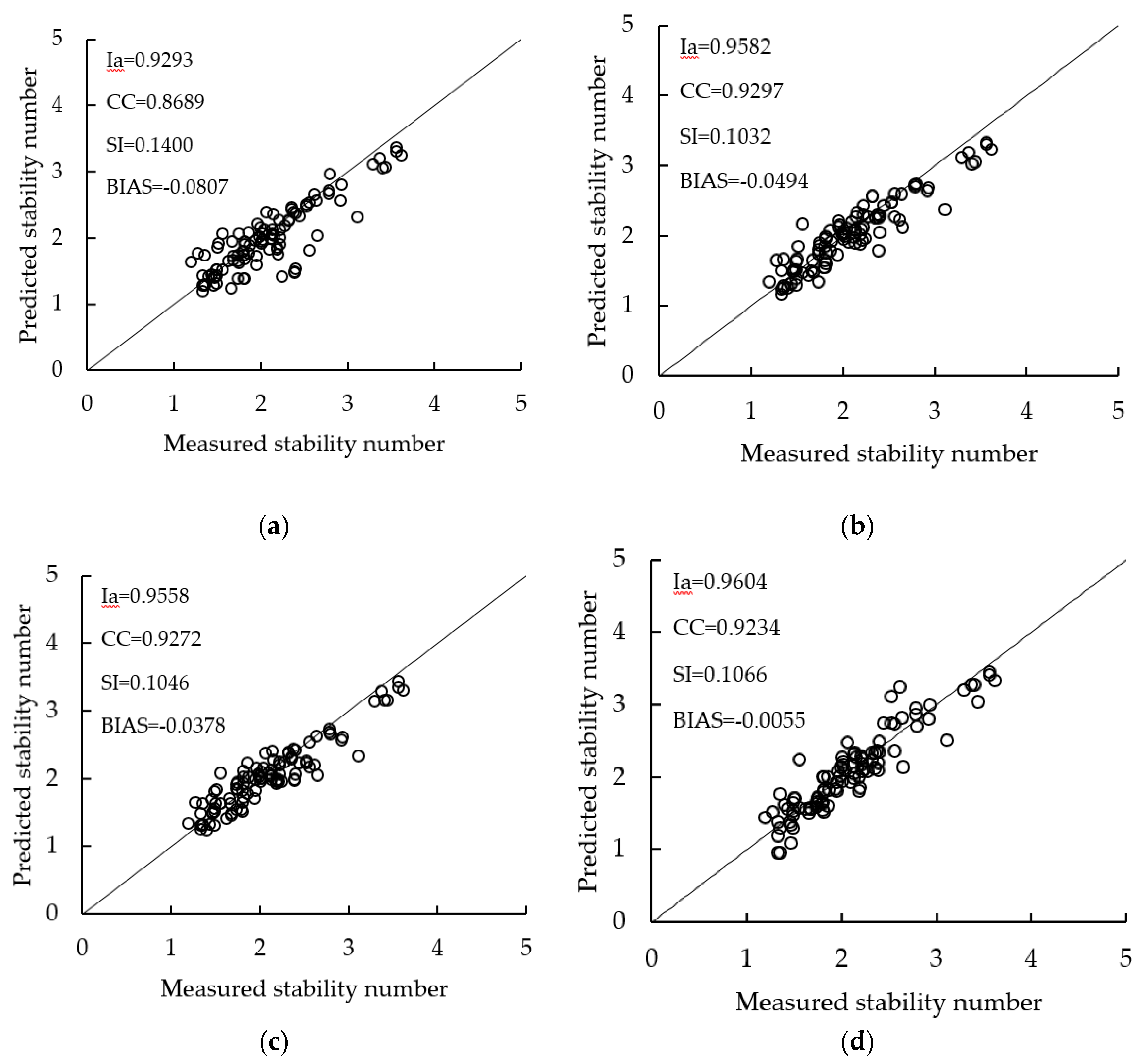
| Methods | BIAS | SI | CC | Ia |
|---|---|---|---|---|
| VM | −0.0807 | 0.1400 | 0.8689 | 0.9293 |
| EB | −0.0494 | 0.1032 | 0.9297 | 0.9582 |
| GPM1 | −0.0378 | 0.1046 | 0.9272 | 0.9558 |
| ELM(M1) | −0.0055 | 0.1066 | 0.9234 | 0.9604 |
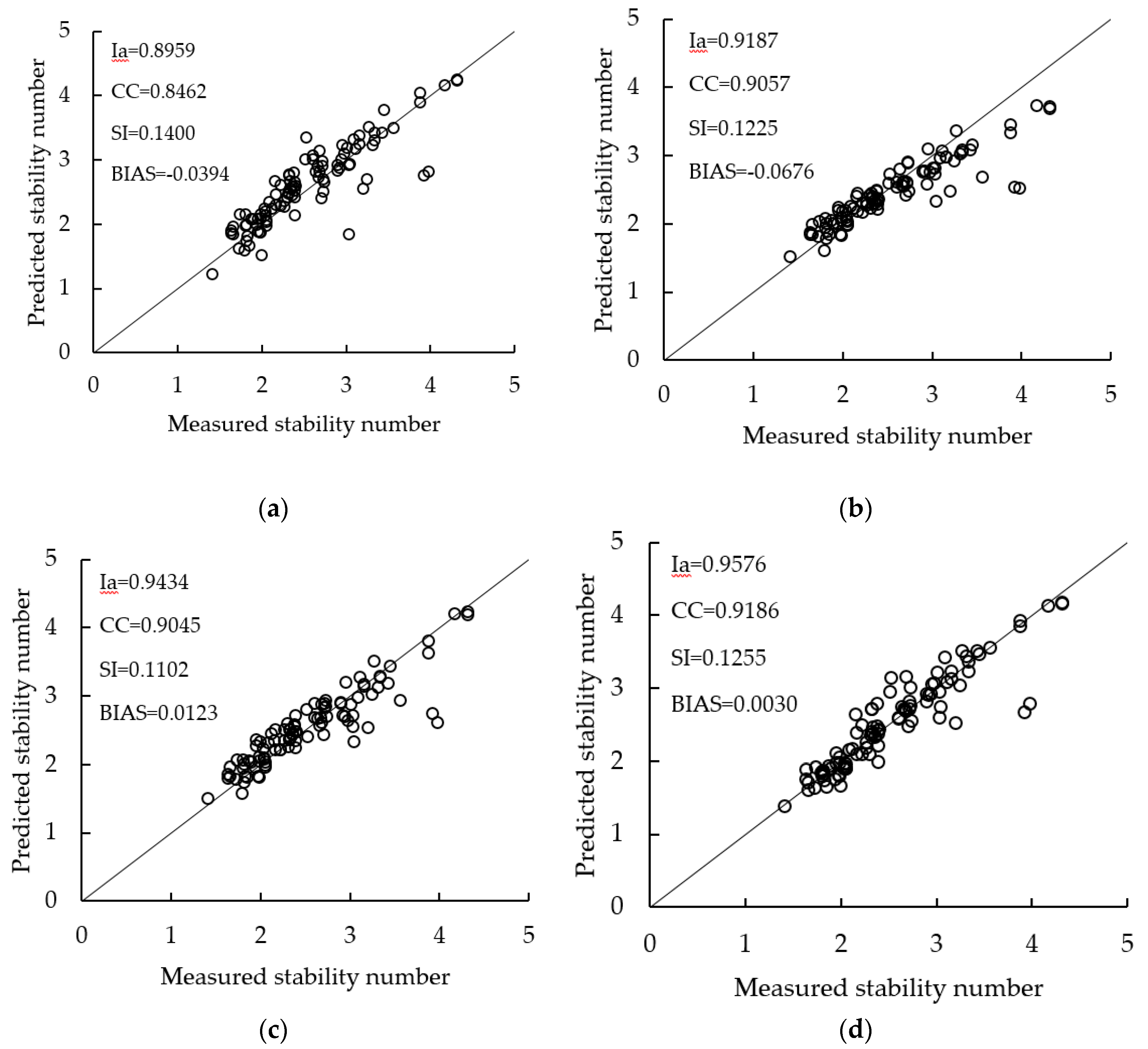
| Methods | BIAS | SI | CC | Ia |
|---|---|---|---|---|
| VM | −0.0394 | 0.1400 | 0.8462 | 0.8959 |
| EB | −0.0676 | 0.1225 | 0.9057 | 0.9189 |
| GPM1 | 0.0123 | 0.1102 | 0.9045 | 0.9434 |
| ELM(M2) | 0.0030 | 0.1022 | 0.9186 | 0.9576 |
| Researchers | CC | Ia | Training Data | Input Parameters | Testing Data | |
|---|---|---|---|---|---|---|
| Mase, Sakamoto and Sakai [24] | 0.91 | 100 | 6 | No | ||
| Dong and Park [12] | I | 0.914 | 100 | 6 | 641 | |
| II | 0.906 | 100 | 5 | 641 | ||
| III | 0.902 | 100 | 6 | 641 | ||
| IV | 0.915 | 100 | 7 | 641 | ||
| V | 0.952 | 100 | 8 | 641 | ||
| Kim, Dong and Chang [15] | I | 0.905 | 0.948 | 207 | 5 | 119 |
| II | 0.913 | 0.954 | 201 | 5 | 114 | |
| Erdik [16] | FL | 0.945 | 579 | 6 | 579 | |
| Balas, Koç and Tür [13] | HNN-1 | 0.936 | 180 (PCA) | 5 | 76 | |
| HNN-2 | 0.927 | 180 (PCA) | 4 | 76 | ||
| Koç and Balas [17] | GA-FNN | 0.932 | 166 (PCA) | 5 | 42 | |
| HGA-FNN | 0.947 | 166 (PCA) | 5 | 42 | ||
| Etemad-Shahidi and Bonakdar [8] | MT1 | 0.931 | 0.97 | 386 | 5 | 193 |
| MT2 | 0.968 | 0.976 | 386 | 6 | 193 | |
| Koc, Balas and Koc [23] | GPM1 | 0.98 | 207 | 7 | 372 | |
| GPM2 | 0.95 | 40 | 7 | 22 | ||
| GPM3 | 0.989 | 207 | 7 | 372 | ||
| GPM4 | 0.991 | 40 | 7 | 22 | ||
| VM | 0.969 | 372 | ||||
| VM | 0.65 | 22 | ||||
| Current Study | ELM-M1 | 0.923 | 0.960 | 100 | 5 | 100 |
| ELM-M2 | 0.919 | 0.958 | 100 | 5 | 100 | |
© 2019 by the authors. Licensee MDPI, Basel, Switzerland. This article is an open access article distributed under the terms and conditions of the Creative Commons Attribution (CC BY) license (http://creativecommons.org/licenses/by/4.0/).
Share and Cite
Wei, X.; Liu, H.; She, X.; Lu, Y.; Liu, X.; Mo, S. Stability Assessment of Rubble Mound Breakwaters Using Extreme Learning Machine Models. J. Mar. Sci. Eng. 2019, 7, 312. https://doi.org/10.3390/jmse7090312
Wei X, Liu H, She X, Lu Y, Liu X, Mo S. Stability Assessment of Rubble Mound Breakwaters Using Extreme Learning Machine Models. Journal of Marine Science and Engineering. 2019; 7(9):312. https://doi.org/10.3390/jmse7090312
Chicago/Turabian StyleWei, Xianglong, Huaixiang Liu, Xiaojian She, Yongjun Lu, Xingnian Liu, and Siping Mo. 2019. "Stability Assessment of Rubble Mound Breakwaters Using Extreme Learning Machine Models" Journal of Marine Science and Engineering 7, no. 9: 312. https://doi.org/10.3390/jmse7090312
APA StyleWei, X., Liu, H., She, X., Lu, Y., Liu, X., & Mo, S. (2019). Stability Assessment of Rubble Mound Breakwaters Using Extreme Learning Machine Models. Journal of Marine Science and Engineering, 7(9), 312. https://doi.org/10.3390/jmse7090312