A Nourishment Performance Index for Beach Erosion/Accretion at Saadiyat Island in Abu Dhabi


 ,
,  and
and 
Abstract
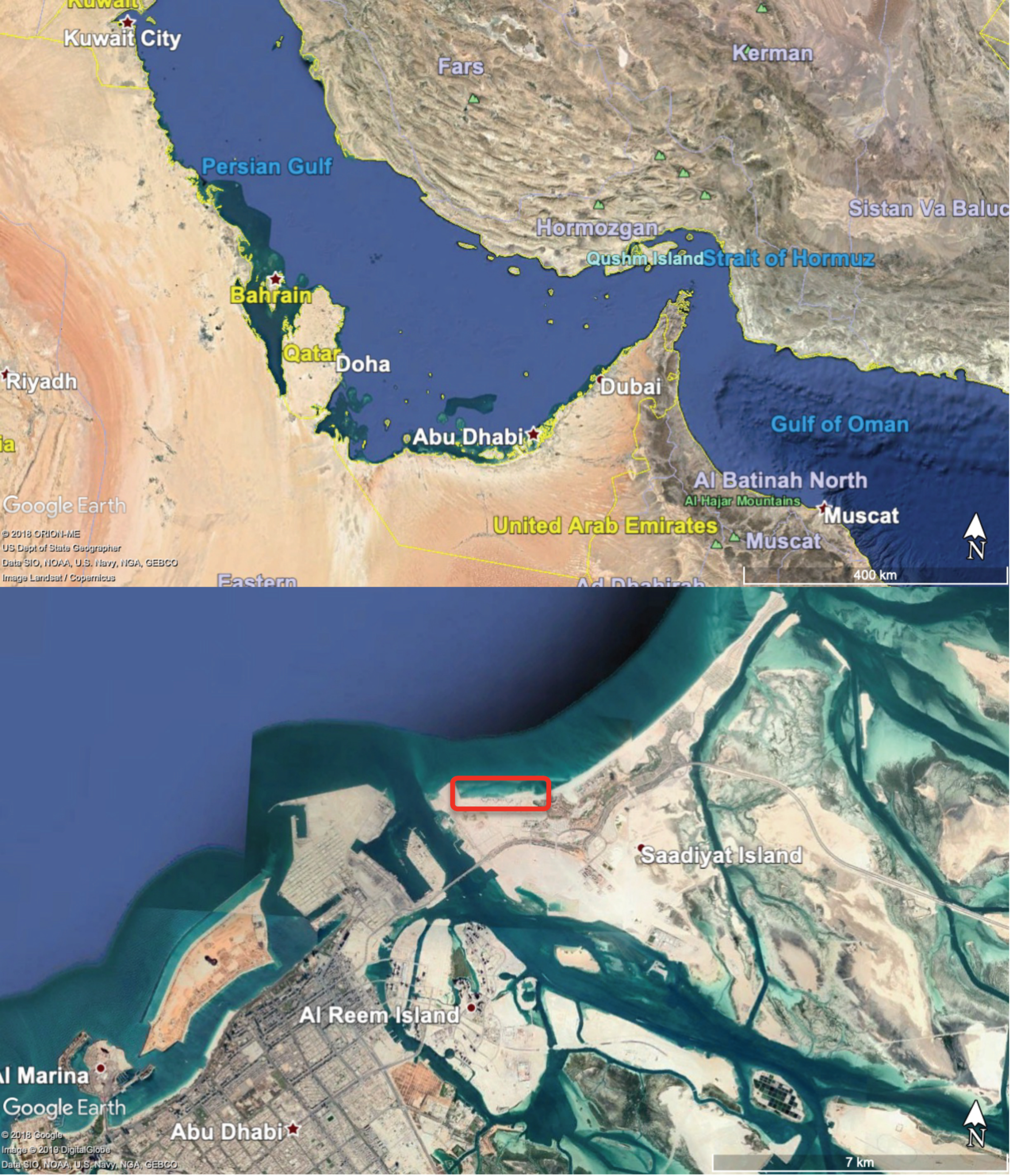
1. Introduction
2. Materials and Methods
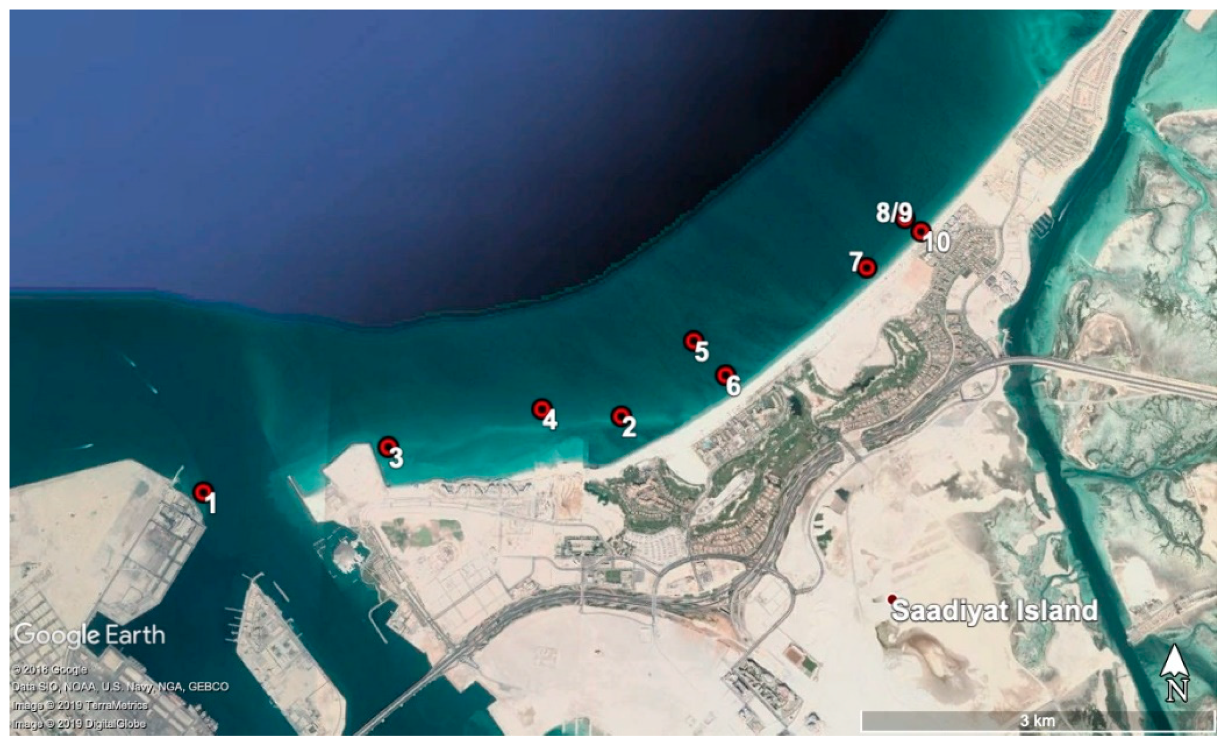
2.1. Sediment Characteristics
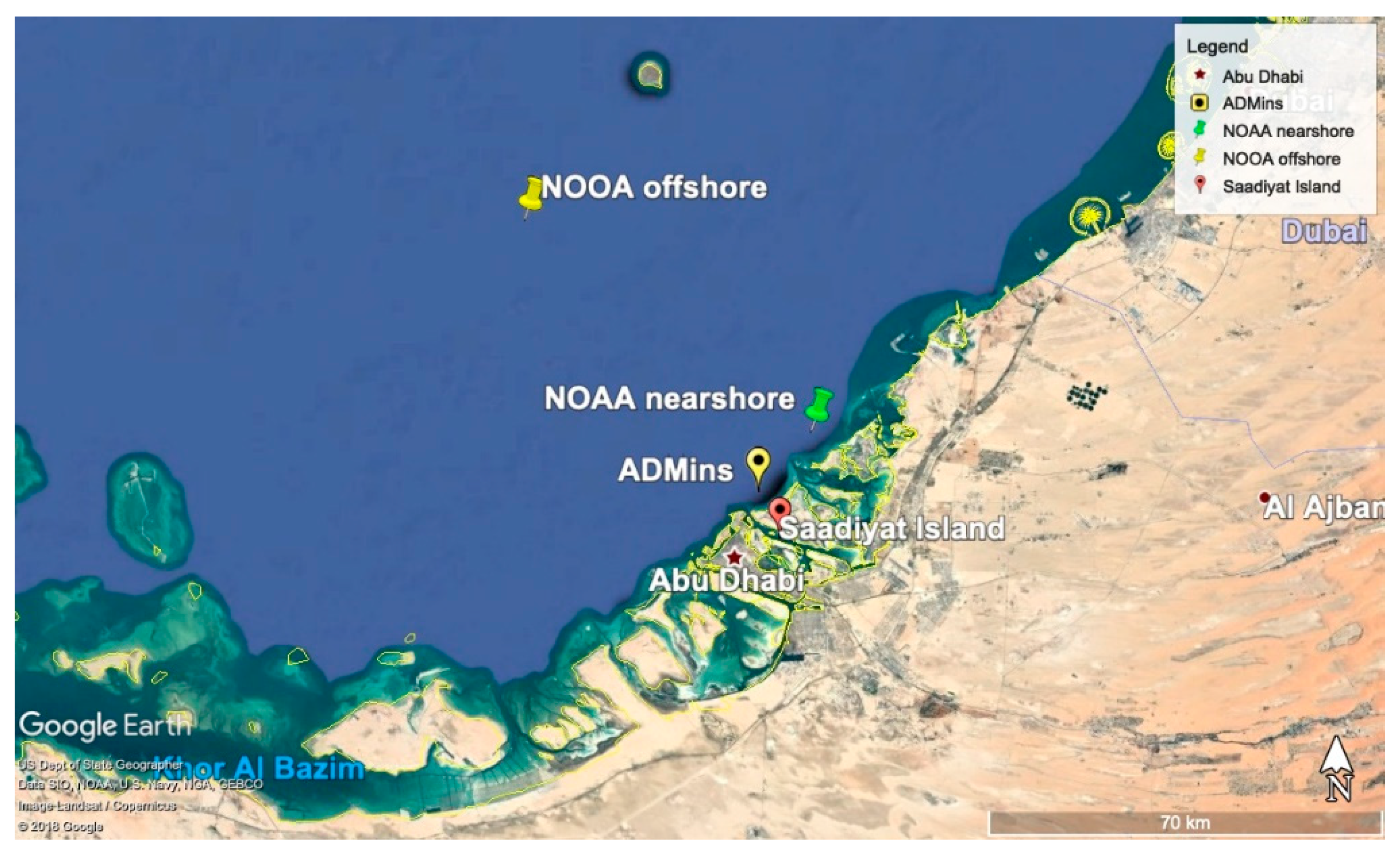
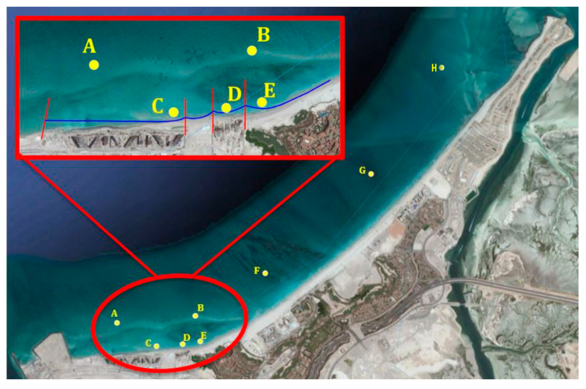
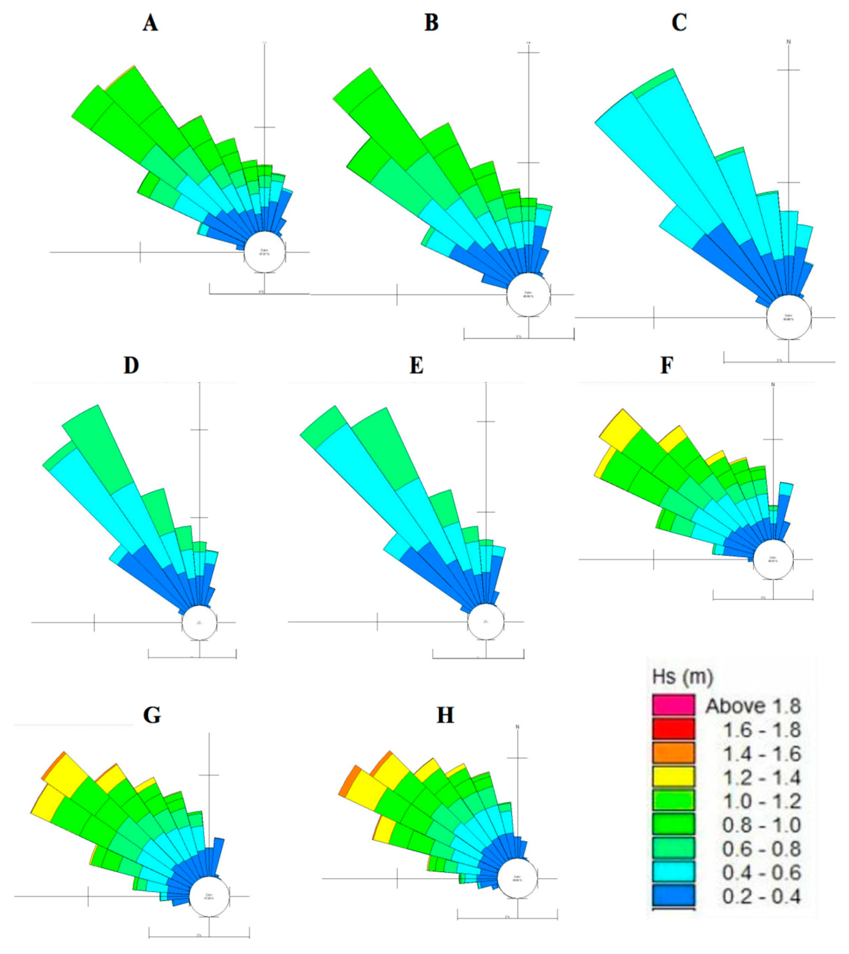
2.2. Local Wave Climate
2.3. Morphodynamic Modelling Techniques
2.3.1. Overview of Popular Commercial Software
2.3.2. GSb Model Description
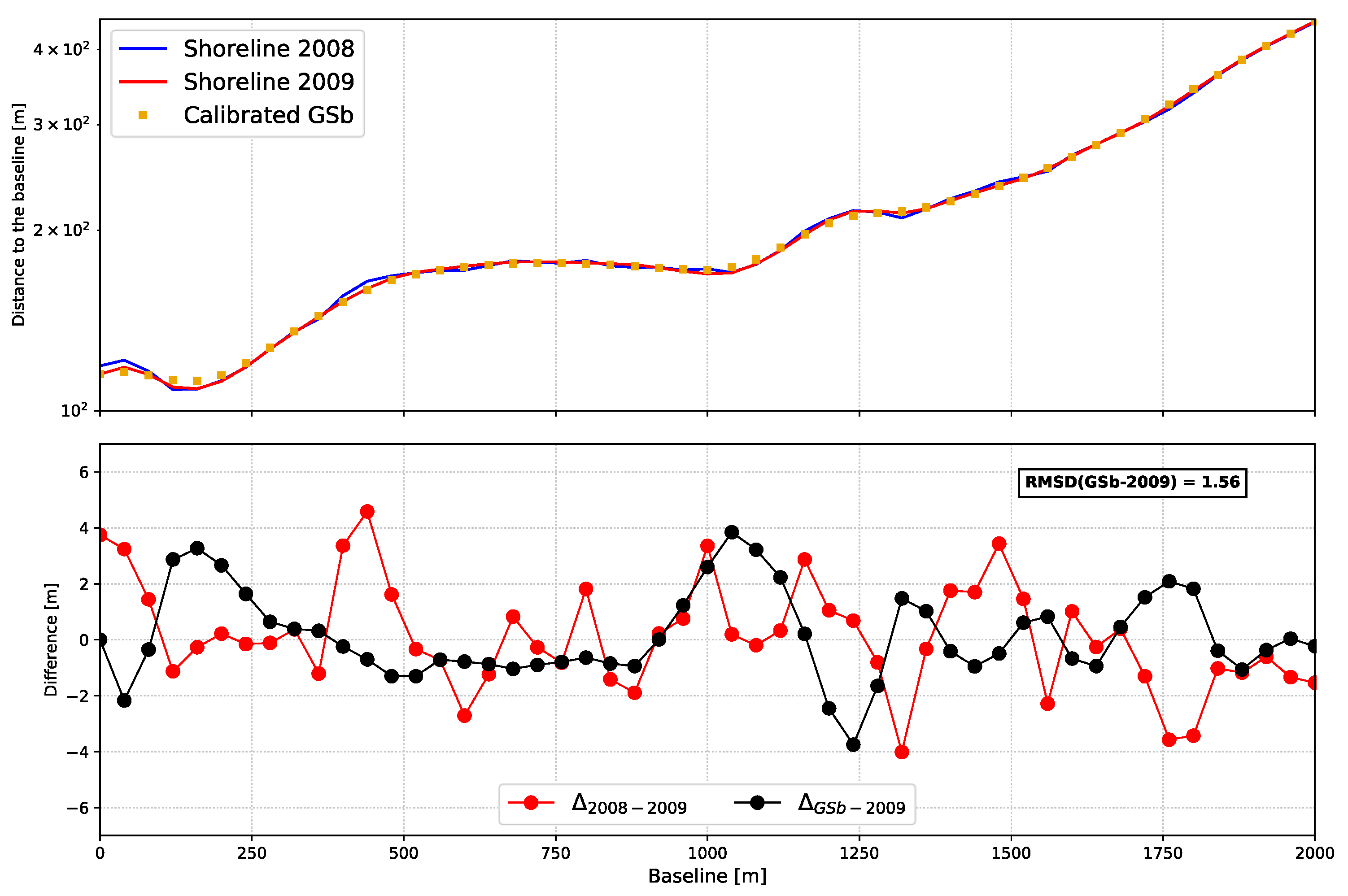
2.3.3. Calibration of the GSB Model
2.4. Other Numerical Models: Ghost
2.5. The Nourishment Performance Index
3. Results
3.1. Nearshore Wave Climate
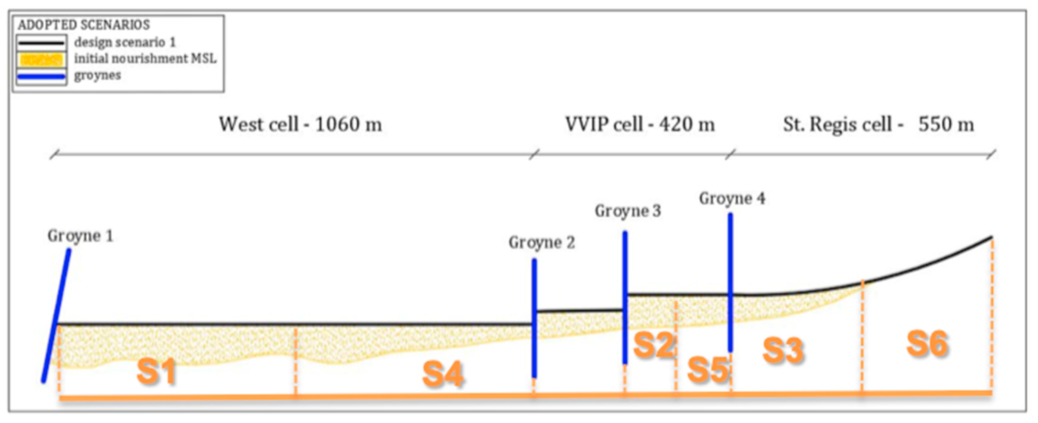
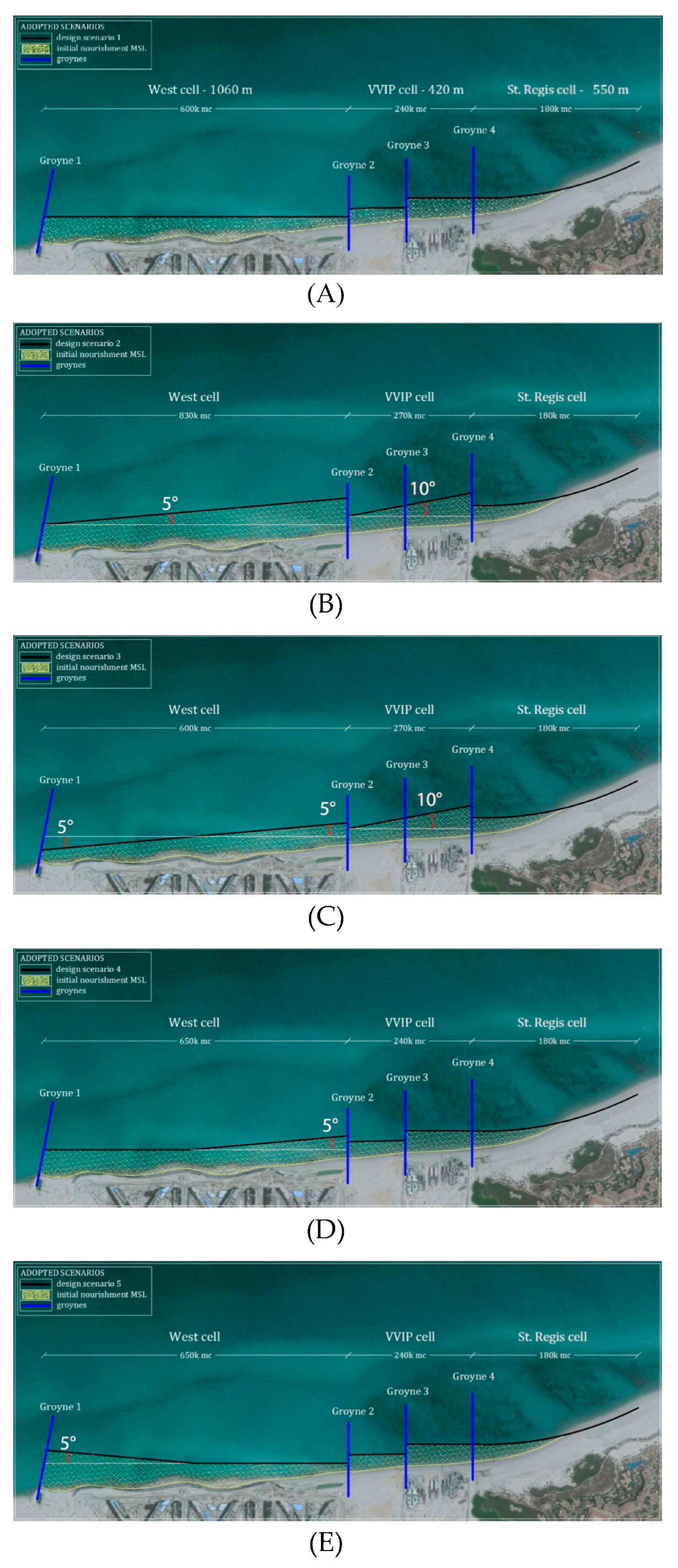
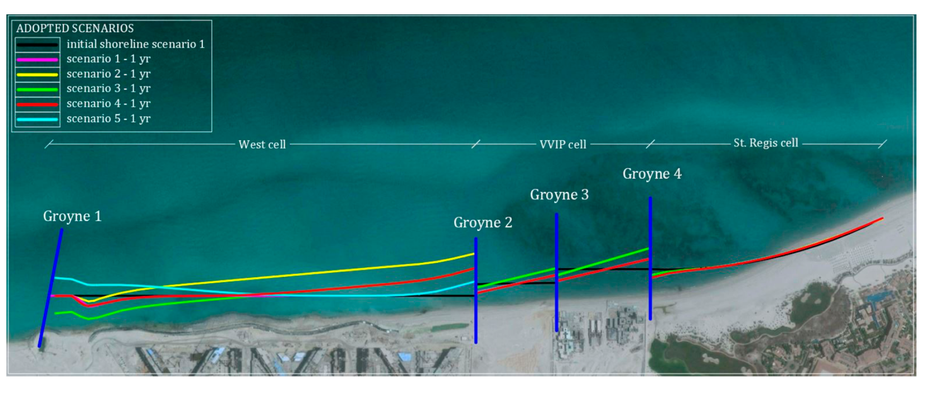
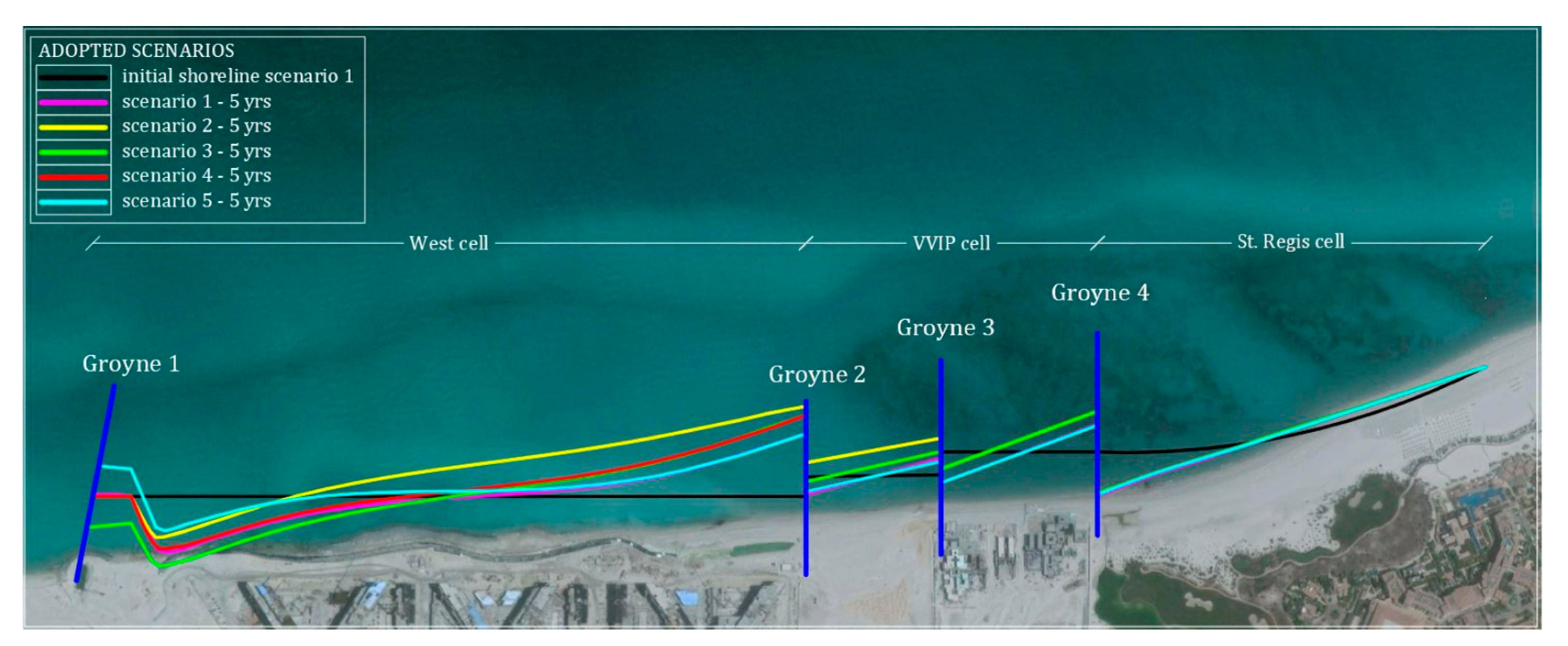
3.2. Shoreline Design Scenarios
3.3. Shoreline Evolution for the Design Scenarios
3.4. The Nourishment Performance Index
4. Discussion
5. Conclusions
Author Contributions
Funding
Acknowledgments
Conflicts of Interest
References
- Hallermeier, R.J. A Profile Zonation for Seasonal Sand Beaches from Wave Climate. Coast. Eng. 1981, 4, 253–277. [Google Scholar] [CrossRef]
- Goda, Y. Random Seas and Design of Maritime Structures, 3rd ed.; Advanced Series on Ocean Engineering; World Scientific: Singapore, 2010. [Google Scholar]
- Tomasicchio, G.R.; D’Alessandro, F. Wave energy transmission through and over low crested breakwaters. J. Coast. Res. 2013, 1, 398–403. [Google Scholar] [CrossRef]
- USACE—United States Army, Corps of Engineers. Shore Protection Manual; Department of the Army, Waterways Experiment Station, Corps of Engineers, Coastal Engineering Research Center: Washington, DC, USA, 1984.
- Van der Meer, J.W. Rock Slopes and Gravel Beaches under Wave Attack. Ph.D. Thesis, Delft University of Technology, Delft, The Netherlands, 1988. [Google Scholar]
- Folk, R.L.; Ward, W.C. Brazos River Bar: A Study in the Significance of Grain Size Parameters. J. Sediment. Petrol. 1957, 27, 3–26. [Google Scholar] [CrossRef]
- Ojeda, E.; Ruessink, B.G.; Guillen, J. Morphodynamic response ofa two-barred beach to a shoreface nourishment. Coast. Eng. 2008, 55, 1185–1196. [Google Scholar] [CrossRef]
- Stauble, D.K. A review of the role of grain size in beach nourishment projects. In Proceedings of the National Conference on Beach Preservation Technology, Destin, FL, USA, 2–4 February 2005. [Google Scholar]
- Utizi, K.; Corbau, C.; Rodella, I.; Nannini, S.; Simeoni, U. A mixed solution for a highly protected coast (Punta Marina, Northern Adriatic Sea, Italy). Mar. Geol. 2016, 381, 114–127. [Google Scholar] [CrossRef]
- Hamza, W.; Lusito, L.; Ligorio, F.; Tomasicchio, G.R.; D’Alessandro, F. Wave Climate at Shallow Waters along the Abu Dhabi Coast. Water 2018, 10, 985. [Google Scholar] [CrossRef]
- Saha, S.; Moorthi, S.; Pan, H.L.; Wu, X.; Wang, J.; Nadiga, S.; Tripp, P.; Kistler, R.; Woollen, J.; Behringer, D.; et al. The NCEP Climate Forecast System Reanalysis. Bull. Am. Meteorol. Soc. 2010, 91, 1015–1057. [Google Scholar] [CrossRef]
- Amante, C.; Eakins, B.W. ETOPO1 1 Arc-Minute Global Relief Model: Procedures, Data Sources and Analysis. In NOAA Technical Memorandum NESDIS; NGDC-24; National Geophysical Data Center: Boulder, CO, USA, 2009; p. 19. [Google Scholar]
- WAVEWATCH III 30-Year Hindcast Wave Model Developed by NOAA (Phase 2). Available online: http://polar.ncep.noaa.gov/waves/hindcasts/nopp-phase2.php (accessed on 4 October 2017).
- The Climate Forecast System Reanalysis (1979–2010). Available online: http://cfs.ncep.noaa.gov/cfsr/ (accessed on 4 October 2018).
- Syvitski, J.P.M.; Slingerland, R.L.; Burgess, P.; Murray, A.B.; Wiberg, P.; Tucker, G.; Voinov, A. Morphodynamic models: An overview. In River, Coastal and Estuarine Morphodynamics: RCEM 2009; Vionnet, C.A., Garcia, M.H., Latrubesse, E.M., Perillo, G.M.E., Eds.; Taylor & Francis: London, UK, 2010; pp. 3–20. [Google Scholar]
- Short, A.D.; Jackson, D.W.T. Beach Morphodynamics. In Treatise on Geomorphology; Shroder, J.F., Ed.; Academic Press: San Diego, CA, USA, 2013; Volume 10, pp. 106–129. [Google Scholar]
- Roelvink, D.; Reniersc, A.; van Dongeren, A.; de Vries, J.V.T.; McCall, R.; Lescinski, J. Modelling storm impacts on beaches, dunes and barrier islands. Coast. Eng. 2009, 56, 133–1152. [Google Scholar] [CrossRef]
- Hanson, H.; Kraus, N. GENESIS—Generalised Model for Simulating Shoreline Change; Report TR-CERC 89-19 (Report 1); Coastal and Hydraulic Laboratory, US Army Corps of Engineers: Washington, DC, USA, 1989.
- Larson, M.; Kraus, N.C.; Hanson, H. Simulation of regional longshore sediment transport and coastal evolution—The “CASCADE” model. Coast. Eng. 2002, 2002, 2612–2624. [Google Scholar] [CrossRef]
- GenCade Website. U.S. Army Corps of Engineers. Available online: http://cirp.usace.army.mil/products/gencade.php (accessed on 19 April 2019).
- LITPACK Website. Danish Hydraulics Institute. Available online: https://www.mikepoweredbydhi.com/products/litpack (accessed on 19 April 2019).
- Delft3D Website. Deltares, NL. Available online: https://oss.deltares.nl/web/delft3d (accessed on 19 April 2019).
- Frey, A.E.; Connell, K.J.; Hanson, H.; Larson, M.; Thomas, R.C.; Munger, S.; Zundel, A. GenCade Version 1 Model Theory and User’s Guide; Technology Report ERDC/CHL TR-12-25; U.S. Army Engineer Research and Development Center: Vicksburg, MS, USA, 2012. [Google Scholar]
- Dean, R.G. Equilibrium beach profiles: Characteristics and applications. J. Coast. Res. 1990, 71, 53–84. [Google Scholar]
- Bruun, P. Coast Erosion and the Development of Beach Profiles; US Army Engineer Waterways Experiment Station; Beach Erosion Board Technical Memo: Vicksburg, MA, USA, 1954. [Google Scholar]
- Lamberti, A.; Tomasicchio, G.R. Stone mobility and abrasion on reshaping breakwaters. In Proceedings of the Hornafjörður International Coastal Symposium, Höfn, Iceland, 20–24 June 1994; pp. 723–735. [Google Scholar]
- Lamberti, A.; Tomasicchio, G.R. Stone mobility and longshore transport at reshaping breakwaters. Coast. Eng. 1997, 29, 263–289. [Google Scholar] [CrossRef]
- Tomasicchio, G.R.; Archetti, R.; D’Alessandro, F.; Sloth, P. Long-shore transport at berm breakwaters and gravel beaches. In Proceedings of the International Conference Coastal Structures, Venice, Italy, 2–4 July 2007; pp. 65–76. [Google Scholar]
- Tomasicchio, G.R.; D’Alessandro, F.; Barbaro, G.; Malara, G. General longshore transport model. Coast. Eng. 2013, 71, 28–36. [Google Scholar] [CrossRef]
- Tomasicchio, G.R.; D’Alessandro, F.; Barbaro, G.; Musci, E.; De Giosa, T.M. Longshore transport at shingle beaches: An independent verification of the general model. Coast. Eng. 2015, 104, 69–75. [Google Scholar] [CrossRef]
- Tomasicchio, G.R.; D’Alessandro, F.; Barbaro, G.; Ciardulli, F.; Francone, A.; Mahmoudi Kurdistani, S. General model for estimation of longshore transport at shingle/mixed beaches. In Proceedings of the 35th International Conference on Coastal Engineering, Antalya, Turkey, 17–20 November 2016. [Google Scholar]
- Tomasicchio, G.R.; D’Alessandro, F.; Frega, F.; Francone, A.; Ligorio, F. Recent improvements for estimation of longshore transport. Ital. J. Eng. Geol. Environ. 2018. [Google Scholar] [CrossRef]
- Whitford, D.J.; Thornton, E.B. Comparison of wind and wave forcing of longshore currents. Cont. Shelf Res. 1993, 13, 1205–1218. [Google Scholar] [CrossRef]
- Baldock, T.E.; Huntley, D.A. Long-wave forcing by the breaking of random gravity waves on a beach. Proceedings of the Royal Society of London. Series A Math. Phys. Eng. Sci. 2002, 458. [Google Scholar] [CrossRef]
- Abessolo Ondoa, G.; Bonou, F.; Tomety, F.S.; du Penhoat, Y.; Perret, C.; Degbe, C.G.E.; Almar, R. Beach Response to Wave Forcing from Event to Inter-Annual Time Scales at Grand Popo, Benin (Gulf of Guinea). Water 2017, 9, 447. [Google Scholar] [CrossRef]
- Ozasa, H.; Brampton, A.H. Mathematical modeling of beaches backed by seawalls. Coast. Eng. 1980, 4, 47–64. [Google Scholar] [CrossRef]
- Medellín, G.; Torres-Freyermuth, A.; Tomasicchio, G.R.; Francone, A.; Tereszkiewicz, P.A.; Lusito, L.; Palemón-Arcos, L.; López, J. Field and Numerical Study of Resistance and Resilience on a Sea Breeze Dominated Beach in Yucatan (Mexico). Water 2018, 10, 1806. [Google Scholar] [CrossRef]
- Carci, E.; Rivero, F.J.; Burchart, H.Y.; Maciñeira, E. The use of numerical modeling in the planning of physical model tests in a multidirectional wave basin. In Proceedings of the 28th International Coastal Engineering Conference, Cardiff, UK, 7–12 July 2002; pp. 485–494. [Google Scholar]
- Rivero, F.J.; Arcilla, A.S.; Carci, E. Implementation of diffraction effects in the wave energy conservation equation. In Proceedings of the IMA Conference on Wind-Over-Waves Couplings: Perspectives and Prospects, Salford, UK, 8–10 April 1997. [Google Scholar]
- Rivero, F.J.; Arcilla, A.S.; Carci, E. An analysis of diffraction in spectral wave models. In Proceedings of the 3rd International Symposium of Ocean Wave Measurement and Analysis, Waves 97, Reston, Virginia Beach, VA, USA, 3–7 November 1997; pp. 431–445. [Google Scholar]
- Lin, L.; Demirbilek, Z. Evaluation of Two Numerical Wave Models with Inlet Physical Model. J. Waterw. Port Coast. Ocean Eng. 2005, 131, 149–161. [Google Scholar] [CrossRef]
- IISD—International Institute of Sustainable Development. Our Common Future; Report of the World Commission on Environment and Development; IISD: New York, NY, USA, 1987. [Google Scholar]
- Pantusa, D.; D’Alessandro, F.; Riefolo, L.; Principato, F.; Tomasicchio, G.R. Application of a Coastal Vulnerability Index. A Case Study along the Apulian Coastline, Italy. Water 2018, 10, 1218. [Google Scholar]
- SUSTAIN Project. Measuring Coastal Sustainability; A Guide for the Self-Assessment of Sustainability Using Indicators and a Means of Scoring Them; Project Report; Coastal and Marine Union—EUCC: Leiden, The Netherlands, 2010; p. 32. [Google Scholar]
- Fraser, E.D.; Dougill, A.J.; Mabee, W.E.; Reed, M.; McAlpine, P. Bottom up and top down: Analysis of participatory processes for sustainability index identification as a pathway to community empowerment and sustainable environmental management. J. Environ. Manag. 2006, 78, 114–127. [Google Scholar] [CrossRef] [PubMed]
- Niemeijer, D. Developing Indicators for environmental policy: Data-driven and theory-driven approaches examined by example. Environ. Sci. Policy 2002, 5, 91–103. [Google Scholar] [CrossRef]


| ID | Location | Weight (%) Passing Each Mesh (μm) | Sand Classification | ||||||||||
|---|---|---|---|---|---|---|---|---|---|---|---|---|---|
| Coordinates | Water Depth (m) | 5 μm | 10 μm | 18 μm | 35 μm | 60 μm | 120 μm | 230 μm | >230 μm | Type | |||
| 1 | 54°23′10″ E | 24°32′18″ N | 2 | - | 0.4% | 0.4% | 12.2% | 61.8% | 22.0% | 2.3% | 0.9% | 0.44 | Medium |
| 2 | 54°25′20″ E | 24°32′40″ N | 2 | - | 0.2 | 1.0 | 4.2 | 14.7 | 63.1 | 16.1 | 0.7 | 0.26 | Medium |
| 3 | 54°24′07″ E | 24°32′31″ N | 2 | - | 0.2 | 0.5 | 5.2 | 30.3 | 61.3 | 1.6 | 0.9 | 0.33 | Medium |
| 4 | 54°24′55″ E | 24°32′42″ N | 2 | - | 0.0 | 0.1 | 1.8 | 17.8 | 71.1 | 8.6 | 0.6 | 0.27 | Medium |
| 5 | 54°25′43″ E | 24°33′02″ N | 3 | - | 0.5 | 7.0 | 33.5 | 49.0 | 9.3 | 0.4 | 0.3 | 0.65 | Coarse |
| 6 | 54°25′53″ E | 24°32′52″ N | 1 | - | 0.3 | 1.4 | 7.5 | 37.7 | 40.8 | 11.4 | 0.9 | 0.34 | Medium |
| 7 | 54°26′39″ E | 24°33′24″ N | 2 | - | 0.1 | 0.2 | 0.6 | 1.0 | 34.8 | 59.8 | 3.5 | 0.16 | Fine |
| 8 | 54°26′52″ E | 24°33′39″ N | 2 | - | 0.3 | 0.4 | 0.9 | 7.2 | 27.1 | 57.7 | 6.4 | 0.16 | Fine |
| 9 | 54°26′52″ E | 24°33′39″ N | 2 | - | 0.1 | 0.5 | 2.1 | 9.5 | 59.5 | 27.7 | 0.6 | 0.22 | Fine |
| 10 | 54°26′57″ E | 24°33′35″ N | 2 | - | 0.0 | 0.4 | 2.2 | 32.3 | 54.7 | 9.9 | 0.5 | 0.30 | Medium |
| Instrument | Longitude (E) | Latitude (N) | Water Depth (m) |
|---|---|---|---|
| 03 (ADMins) | 54°24′29.52″ | 24°34′17.04″ | 6 |
| 04 | 54°16′39.72″ | 24°44′31.56″ | 18 |
| Scenarios | Sand Volume (×103 m3) | ||
|---|---|---|---|
| West Cell | VVIP Cell | St. Regis Cell | |
| 1 | 600 | 240 | 180 |
| 2 | 830 | 270 | 180 |
| 3 | 600 | 270 | 180 |
| 4 | 650 | 240 | 180 |
| 5 | 650 | 270 | 180 |
| Scenarios | Sand Volume (×103 m3) | Max Recession after 1 year (m) | Max Accretion after 1 year (m) | ||||||
|---|---|---|---|---|---|---|---|---|---|
| West Cell | VVIP Cell | St. Regis Cell | S1 | S2 | S3 | S4 | S5 | S6 | |
| 1 | 600 | 240 | 180 | 26 | 20 | 21 | 20 | 25 | 4 |
| 2 | 830 | 270 | 180 | 20 | 13 | 31 | 44 | 16 | 4 |
| 3 | 600 | 270 | 180 | 20 | 13 | 31 | 30 | 16 | 4 |
| 4 | 650 | 240 | 180 | 26 | 20 | 21 | 30 | 25 | 4 |
| 5 | 650 | 270 | 180 | 10 | 20 | 21 | 20 | 25 | 4 |
| Scenarios | Sand Volume (×103 m3) | Max Recession after 5 years (m) | Max Accretion after 5 years (m) | ||||||
|---|---|---|---|---|---|---|---|---|---|
| West Cell | VVIP Cell | St. Regis Cell | S1 | S2 | S3 | S4 | S5 | S6 | |
| 1 | 600 | 240 | 180 | 80 | 27 | 62 | 75 | 39 | 14 |
| 2 | 830 | 270 | 180 | 65 | 22 | 77 | 71 | 29 | 14 |
| 3 | 600 | 270 | 180 | 63 | 22 | 77 | 79 | 24 | 14 |
| 4 | 650 | 240 | 180 | 79 | 27 | 62 | 79 | 39 | 14 |
| 5 | 650 | 270 | 180 | 85 | 27 | 61 | 76 | 39 | 14 |
| West Cell | VVIP Cell | St. Regis Cell | ||||||||||
|---|---|---|---|---|---|---|---|---|---|---|---|---|
| Recession (m2) | Sand Volume ×103 (m3) | Recession (m2) | NPI | NPI Increase (%) | Sand volume ×103 (m3) | Recession (m2) | NPI | NPI Increase (%) | Sand Volume ×103 (m3) | NPI | NPI Increase (%) | |
| 1 | 600 | 2227 | 75 | reference | 240 | 2685 | 25 | reference | 180 | 1110 | 45 | reference |
| 2 | 830 | 2394 | 96 | 29 | 270 | 1707 | 44 | 77 | 180 | 638 | 78 | 74 |
| 3 | 600 | 1944 | 86 | 15 | 270 | 1338 | 56 | 126 | 180 | 693 | 72 | 60 |
| 4 | 650 | 2368 | 76 | 2 | 240 | 2712 | 25 | -1 | 180 | 962 | 52 | 15 |
| 5 | 650 | 874 | 207 | 176 | 270 | 2708 | 28 | 12 | 180 | 1140 | 44 | -3 |
| Scenarios (5 years) | Sand Volume ×103 (m3) | Recession (m2) | NPI | NPI Increase (%) | Sand Volume ×103 (m3) | Recession (m2) | NPI | NPI Increase (%) | Sand Volume ×103 (m3) | Recession (m2) | NPI | NPI Increase (%) |
| 1 | 600 | 15,450 | 11 | reference | 240 | 3643 | 18 | reference | 180 | 6175 | 8 | reference |
| 2 | 830 | 13,920 | 17 | 54 | 270 | 1642 | 46 | 150 | 180 | 5625 | 9 | 10 |
| 3 | 600 | 13,017 | 13 | 19 | 270 | 1958 | 38 | 109 | 180 | 5737 | 9 | 8 |
| 4 | 650 | 14,106 | 13 | 19 | 240 | 3615 | 18 | 1 | 180 | 5683 | 9 | 9 |
| 5 | 650 | 13,798 | 13 | 21 | 270 | 3769 | 20 | 9 | 180 | 5856 | 9 | 5 |
© 2019 by the authors. Licensee MDPI, Basel, Switzerland. This article is an open access article distributed under the terms and conditions of the Creative Commons Attribution (CC BY) license (http://creativecommons.org/licenses/by/4.0/).
Share and Cite
Hamza, W.; Tomasicchio, G.R.; Ligorio, F.; Lusito, L.; Francone, A. A Nourishment Performance Index for Beach Erosion/Accretion at Saadiyat Island in Abu Dhabi. J. Mar. Sci. Eng. 2019, 7, 173. https://doi.org/10.3390/jmse7060173
Hamza W, Tomasicchio GR, Ligorio F, Lusito L, Francone A. A Nourishment Performance Index for Beach Erosion/Accretion at Saadiyat Island in Abu Dhabi. Journal of Marine Science and Engineering. 2019; 7(6):173. https://doi.org/10.3390/jmse7060173
Chicago/Turabian StyleHamza, Waleed, Giuseppe Roberto Tomasicchio, Francesco Ligorio, Letizia Lusito, and Antonio Francone. 2019. "A Nourishment Performance Index for Beach Erosion/Accretion at Saadiyat Island in Abu Dhabi" Journal of Marine Science and Engineering 7, no. 6: 173. https://doi.org/10.3390/jmse7060173
APA StyleHamza, W., Tomasicchio, G. R., Ligorio, F., Lusito, L., & Francone, A. (2019). A Nourishment Performance Index for Beach Erosion/Accretion at Saadiyat Island in Abu Dhabi. Journal of Marine Science and Engineering, 7(6), 173. https://doi.org/10.3390/jmse7060173