Article

Stability Assessment of Rubble Mound Breakwaters Using Extreme Learning Machine Models

1
State Key Laboratory of Hydraulics and Mountain River Engineering, College of Water Resource and Hydropower, Sichuan University, Chengdu 610065, China
2
State Key Laboratory of Hydrology-Water Resources and Hydraulic Engineering, Nanjing Hydraulic Research Institute, Nanjing 210029, China
*
Author to whom correspondence should be addressed.
J. Mar. Sci. Eng. 2019, 7(9), 312; https://doi.org/10.3390/jmse7090312
Submission received: 7 August 2019 / Revised: 1 September 2019 / Accepted: 4 September 2019 / Published: 7 September 2019
(This article belongs to the Special Issue Modelling of Harbour and Coastal Structures)

Abstract

:
The stability number of a breakwater can determine the armor unit’s weight, which is an important parameter in the breakwater design process. In this paper, a novel and simple machine learning approach is proposed to evaluate the stability of rubble-mound breakwaters by using Extreme Learning Machine (ELM) models. The data-driven stability assessment models were built based on a small size of training samples with a simple establishment procedure. By comparing them with other approaches, the simulation results showed that the proposed models had good assessment performances. The least user intervention and the good generalization ability could be seen as the advantages of using the stability assessment models.

1. Introduction

The determination of the armor unit’s weight is an important component in the rubble mound breakwater design process, and the armor units play a key role in maintaining the stability of breakwaters under wave attacks. The armor unit’s weight can be computed using the stability number of rubble mound breakwaters, Ns, which is commonly obtained from the Hudson formula [1] or the van der Meer formula [2]. Hudson’s formula is widely used in breakwater design because of its convenient calculation of the unit mass and stability number. Some important physical factors are not involved in the formula, such as the wave period, wave length and the water depth in front of the breakwater, so other researchers did further research. van der Meer [2] proposed the following formula based on more than 300 runs of breakwater experiments under irregular wave attack. Compared to the Hudson formula, more parameters are included in the van der Meer formula (VM formula), such as the number of wave attacks and the breakwater permeability.
N s = 6.2 P 0.18 ( S d N w ) 0.2 1 ξ m   ξ m < ξ c
N s = 1.0 P 0.13 ( S d N w ) 0.2 cot α ξ m p   ξ m ξ c
where P is the permeability of the breakwater, S d is the damage level, N w is the number of wave attacks, ξ m is the surf similarity parameter, ξ c is the transition condition of the surf similarity, and α is the slope angle. Ns can be expressed as follows in the study of van der Meer [2]:
N s = H s Δ D n
where H s is the significant wave height, D n is the nominal median diameter of the stones used in the breakwater, and Δ is the relative mass density, which can be expressed as follows:
Δ = ρ γ ρ
where ρ γ is the stone mass density and ρ is the water mass density.
Over the past decades, van der Meer’s formula has proven to be the most widely used formula to guide rubble mound breakwater design, while at the same time a developed formula was proposed by van der Meer [3,4] to assess the stability of the toe structure of rubble mound breakwaters, based on a new series of experiments. In addition to the studies of Hudson and van der Meer, some other researchers have proposed some novel formulas to assess the stability by analyzing the experimental results, such as [5], Hanzawa, et al. [6], Vidal, et al. [7], Etemad-Shahidi and Bonakdar [8] and Van Gent and Der Werf [9]. Previous studies have shown that the definition equation of the stability number Ns is stable, and that it is a function of the wave height and the relative density and nominal diameter of the stone. Meanwhile, in different studies, the damage condition of the breakwater section used to compute the stability number has various definitions. In the studies of Thompson [10] and Hanzawa [6], a damage parameter was proposed to describe the damage condition of the breakwater section, which was a function of the stone density, stone size, wave height, wave number and erosion area in a cross section, while in the studies of van der Meer [2,3] and Kajima [5], a simple damage level was proposed. A summary of the definitions is listed in Table 1 [11].
Besides the empirical formula, Ns can also be predicted by using the machine learning approaches. In the past two decades, a large and growing body of literature has investigated the machine learning approaches to assess the stability of rubble mound breakwaters, such as Artificial Neural Networks (ANN) [12,13,14,15], Fuzzy Neural Networks (FNN) [16,17], Model Tress (MT) [8,18], Support Vector Machine (SVM) [19,20,21,22], and Genetic Programing (GP) [23]. These studies have shown that the performance of machine learning approaches is better than that of the traditional formulas [23,24]. The study of Balas, Koç and Tür [13] provides new insights into improving the prediction accuracy of ANN models via the principal component analysis, which could reduce the needed amount of training data and transform the original data set into a set of uncorrelated variables that capture all of the variance of the original data set [25], but many methods still suffered from complex establishment procedures and large demands for the training sets’ size. Thus, reducing the parameter counts and the training data size, and simplifying the training process, should be a concern for further research.
The Extreme Learning Machine is a robust machine learning algorithm based on the Single-Hidden Layer Feedforward Network (SLFN) [26], which was very simple in t neural network architecture. Previous studies have shown that the ELM could be used in wide areas, such as classification [27,28,29,30] and regression [31,32,33,34], and that it showed a good generalization performance at fast learning speeds [35]. The main advantage of ELM is that the user-defined parameters for training an assessment ELM model only include the kind of activation function and the number of hidden neurons, which makes the model establishment very convenient; besides, the ELM model can obtain a high prediction accuracy based on a small size of training data sets. Based on this, the ELM method was proposed to develop a novel and simple stability assessment model of rubble mound breakwaters. This is the first study on the application of ELM in the stability assessment of rubble mound breakwaters. Therefore, the findings in this study make a contribution to the stability assessment and to the design of the rubble mound breakwaters.
This paper is organized as follows. The fundamentals of the ELM approach and the model establishment are introduced in Section 2. In Section 3, the application of the ELM approach for the stability assessment of rubble-mound breakwaters is discussed, and a comparison between the ELM approach and other approaches is given. The main findings of this paper are summarized in Section 4.

2. Extreme Learning Machine Models

The Extreme Learning Machine is widely used in regression and classification [36]. However, up to now, few studies involving applications of ELM in coastal engineering have been published. A search of the literature revealed that ELM was once used to predict the sea level, tide, and wave heights [37,38,39,40]. In the following subsection, a brief introduction about the fundamentals of Extreme Learning Machine models is given to clarify the process details of the ELM model establishment. More information about ELM models can be found in Huang, Zhu and Siew [26,35], Huang, Huang, Song and You [36].

2.1. Fundamental of Extreme Learning Machine Model

The goal of the learning process is to find the relation between input training data sets and output training labels. Considering an ELM neural network with n neurons in the input layer, l neurons in the hidden layer, and m neurons in the output layer, the general structure of ELM is shown in Figure 1:
The weight w between the neurons in the input layer and the neurons in the hidden layer can be expressed as:
w = [ ω 11 ω 1 n ω l 1 ω l n ] l × n
where w j i is the weight between the neuron i in the input layer and the neuron j in the hidden layer.
Meanwhile, the weight β between the neurons in the hidden layer and the neurons in the output layer can be expressed as:
β = [ β 11 β 1 m β l 1 β l m ] l × m
where β j m is the weight between the neuron j in the hidden layer and the neuron m in the output layer.
The bias b in the hidden layer is:
b = [ b 1 b 2 b l ]
For the given training samples X and the output matrix Y:
X = [ x 11 x 1 Q x n 1 x n Q ] n × Q
Y = [ y 11 y 1 Q y m 1 y m Q ] m × Q
Assuming that the activation function in the hidden layer was g(x), then the output T is:
T = [ t 1 , t 2 , t Q ] ,   t j = [ t 1 j t m j ] = [ i = 1 l β j 1 g ( w i x j + b i ) i = 1 l β i m g ( w i x j + b i ) ]   ( j = 1 , 2 , 3 ,   ,   Q )
where ω i = [ ω i 1 , ω i 2 , ω i m , ] , and x j = [ x 1 j , x 2 j , , x n j ] T .
Equation 11 can be rewritten in the following form:
H β = T
where T is the transposed matrix of T. H is the hidden layer output matrix of the neural network, which is as follows:
H ( ω 1 , ω 2 , ω l ,   b 1 , b 2 , b l , x 1 , x 2 , , x Q ) = [ g ( w 1 , b 1 , x 1 ) g ( w l , b l , x 1 ) g ( w 1 , b 1 , x Q ) g ( w l , b l , x Q ) ] Q × l
The minimum norm least-squares solution of min β H β T is unique:
β ^ = H + T
where H + is the Moore-Penrose generalized inverse of the matrix of H.
More details about the ELM theory can be found in the studies of Huang, Zhu and Siew [35], Huang, Huang, Song and You [36].
The activation functions used in this paper are as follows:
Sigmoid function:
g ( w i x + b i ) = 1 1 + ( exp ( w i x + b i ) )
Sin function:
g ( w i x + b i ) = sin ( w i x + b i )
Hardlim function:
g ( w i x + b i ) = { 1   w i x + b i 0 2   w i x + b i < 0
Trigonometric basis function:
g ( w i x + b i ) = { 1 | w i x + b i |   1 w i x + b i 1 0   else
Radial basis function:
g ( w i x + b i ) = exp ( x w i 2 b i 2 )

2.2. Model Establishment

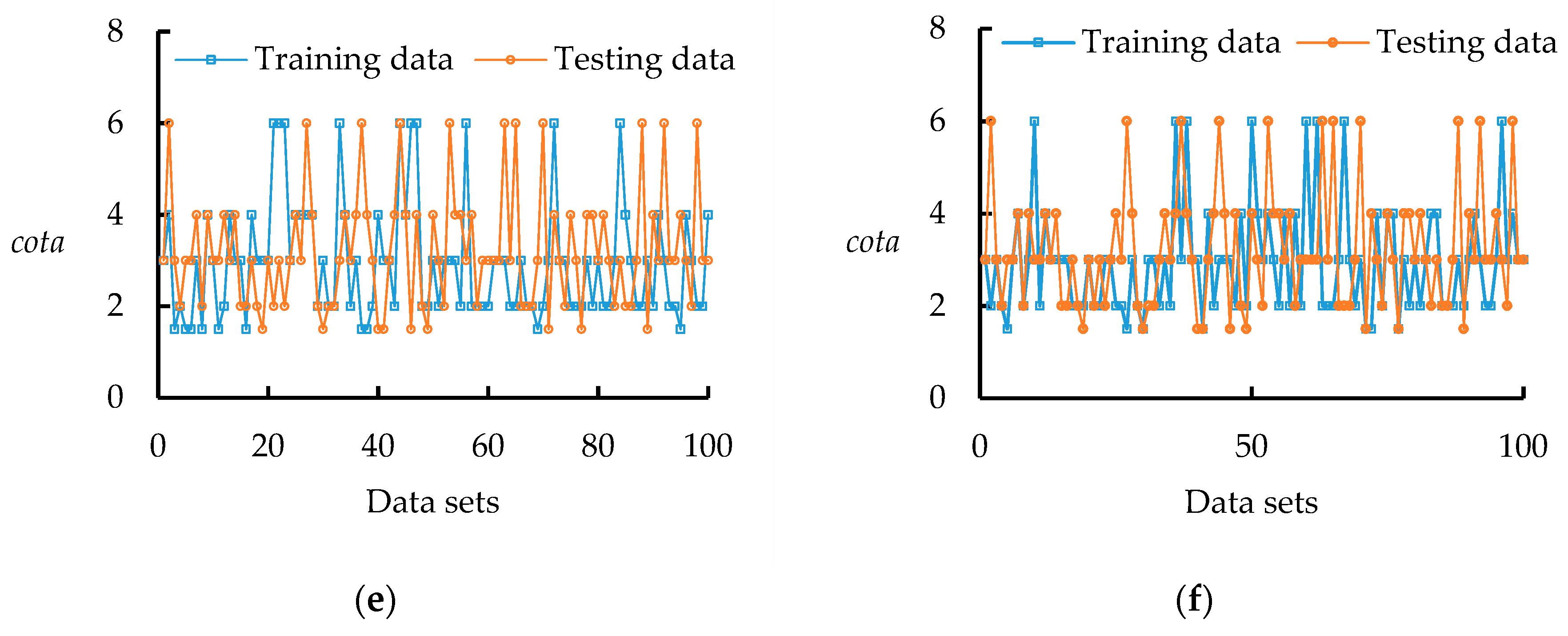
Based on the damage level of the breakwater sections, two ELM models were built to predict the stability number of breakwaters. The first model (M1) was aimed at predicting the stability number of the breakwater sections whose damage level was in the range of 2 to 8. The other model (M2) was aimed at predicting the stability number of the breakwater sections whose damage level was in the range of 8 to 32 (8 was not included). High damage levels (S > 8) are not common in design practice [18]. Basheer and Hajmeer [41] (cited in Balas, Koç and Tür [13]) pointed out that there are no mathematical rules to determine the required amounts of training data and testing data. The number of the training data sets ranges from 90 to 579 in the previous studies discussed earlier. In the current study, 100 data points for training and 100 data points for testing were randomly selected for each model (M1, M2) from the experimental data of van der Meer [2], according to the damage level of the data, which can be found in in the Supplementary Materials. Five parameters we selected as the input nodes: the permeability, damage level, wave attack number, slope angle, and surf similarity parameter. The range of parameters used in the M1 and M2 models were presented in Figure 2 and Table 2.
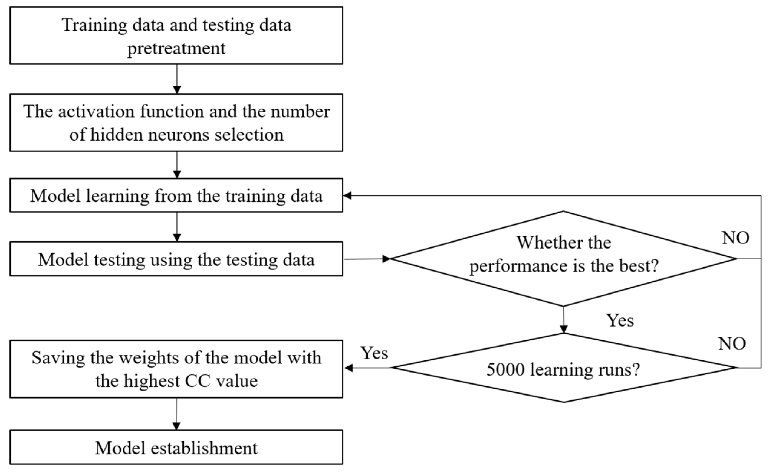
The flow chart of the ELM model establishment is shown in Figure 3. For each model, 5000 learning runs from the training data are necessary before the assessment model establishment. In order to evaluate the assessment performance of these ELM models, the bias (BIAS), correlation coefficient (CC), scatter index (SI) and index of agreement (Ia) are introduced as follows:
B I A S = i = 1 N 1 N ( Y i X i )
S I = 1 N i = 1 N ( Y i X i ) 2 X i ¯
C C = i = 1 N ( X i X ¯ ) ( Y i Y ¯ ) i = 1 N ( X i X ¯ ) 2 i = 1 N ( Y i Y ¯ ) 2
I a = 1 i = 1 N ( Y i X i ) 2 i = 1 N ( | ( Y i X ¯ ) | + | ( X i X ¯ ) | ) 2
where Xi are the measured values, and their average is X ¯ ; Yi are the predicted values, and their average is Y ¯ ; and N is the number of observations.
A search of the literatures shows that the CC parameter was the most widely used index to evaluate the model performances, meanwhile, when the CC value of the model reaches the highest value, the Ia value may not, so in the training process, the value of CC was selected as the only evaluation index of the models. After the training process, the weights of the model with the highest CC value are recorded, which can be used for the stability assessment. The data used for establishing the models is provided in the Supplementary Materials. The weights used in the M1 model and the M2 model are listed in Appendix A. The code used in this paper is provided in Appendix B.

3. Results and Discussion

3.1. The Influence of Hidden Neurons on the Assessment Performance of ELM Models with Different Activation Functions

The assessment performances of the ELM models are mainly determined by the number of the hidden neurons and the activation functions. Low damage levels (S < 8) are more common in the design practice for rubble mound breakwaters, as previously mentioned [18], and the selection of training data has little influence on this issue, so the M1 models (S < 8) were built to research the influence of the hidden neurons and the activation functions on the model performance.
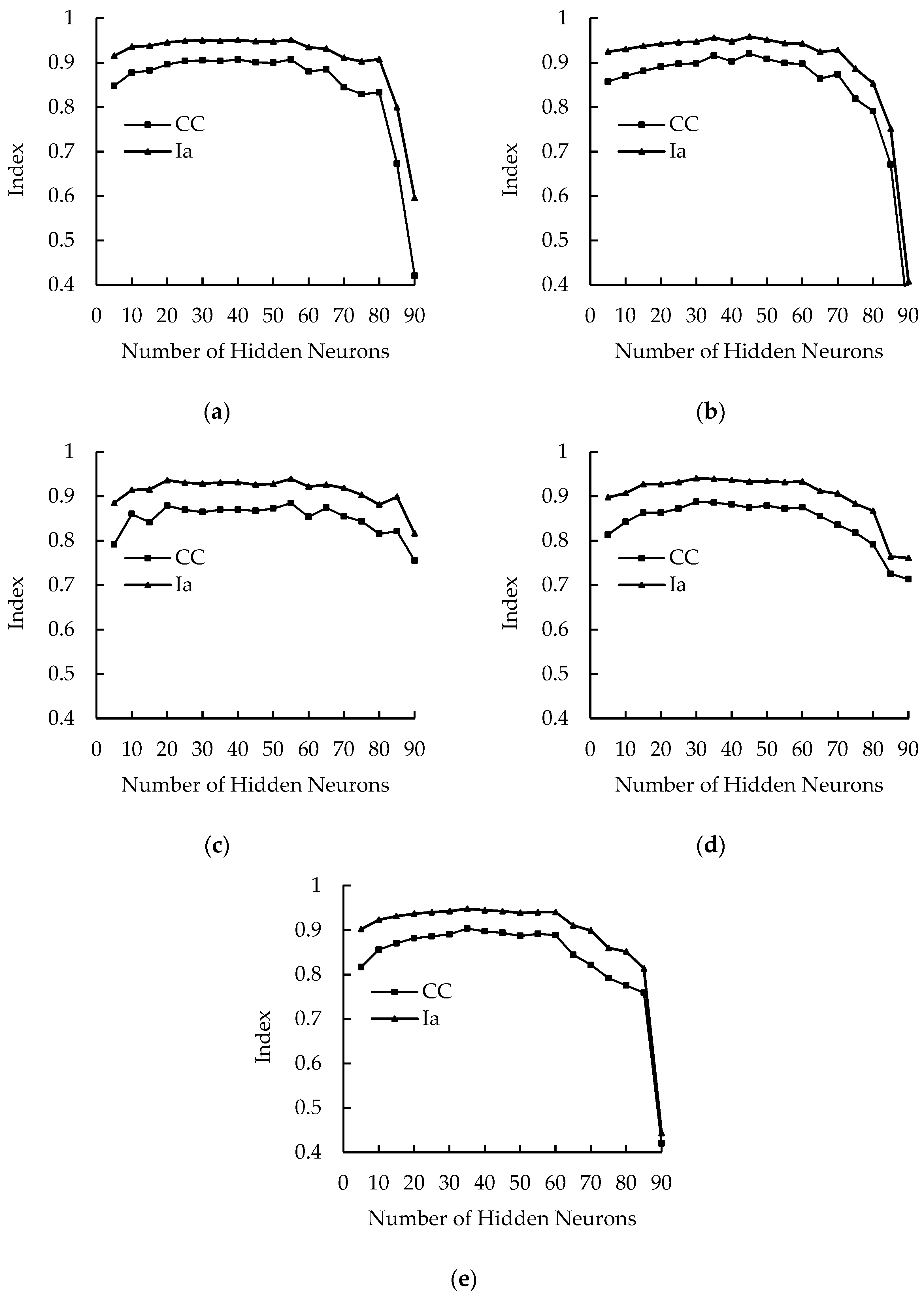
Figure 4 shows the assessment performance of ELM models with different activation functions and different numbers of hidden neurons. The number of hidden neurons of these models were set from 5 to 90 with an interval of 5. It can be seen from the figures that the evaluation criteria CC and Ia are increasing following the addition of hidden neurons when the number of the hidden neurons is within the range of 5 to 20; then, the values of CC and Ia stay relatively constant when the number of the hidden neurons is above 20. The assessment performance criteria have a rapidly decreasing trend as the hidden neurons number increases in the range of 50 to 90, which indicates that too many hidden neurons lead to over-fitting. The models with the best assessment performance were the models built with 40–50 hidden neurons in the hidden layer, no matter what activation function was used in the models. What stands out in Figure 4 is that, for an ELM model with a randomly selected number of hidden neurons from 20 to 50, Ia is no less than 0.9 and CC is no less than 0.85. The selection of the activation function has little influence on the best performance of each model, which is mainly because the training data has few noisy data sets and is pure enough. The simulation results show that the ELM algorithm has a good generalization performance for the stability assessment.
A comparison of these results reveals that the ELM model with the maximum CC and Ia was the model built with 45 hidden neurons and the Sin function. The parameters for the model training and application were determined for these conditions.

3.2. Predicted Performance Comparison of Different Methods

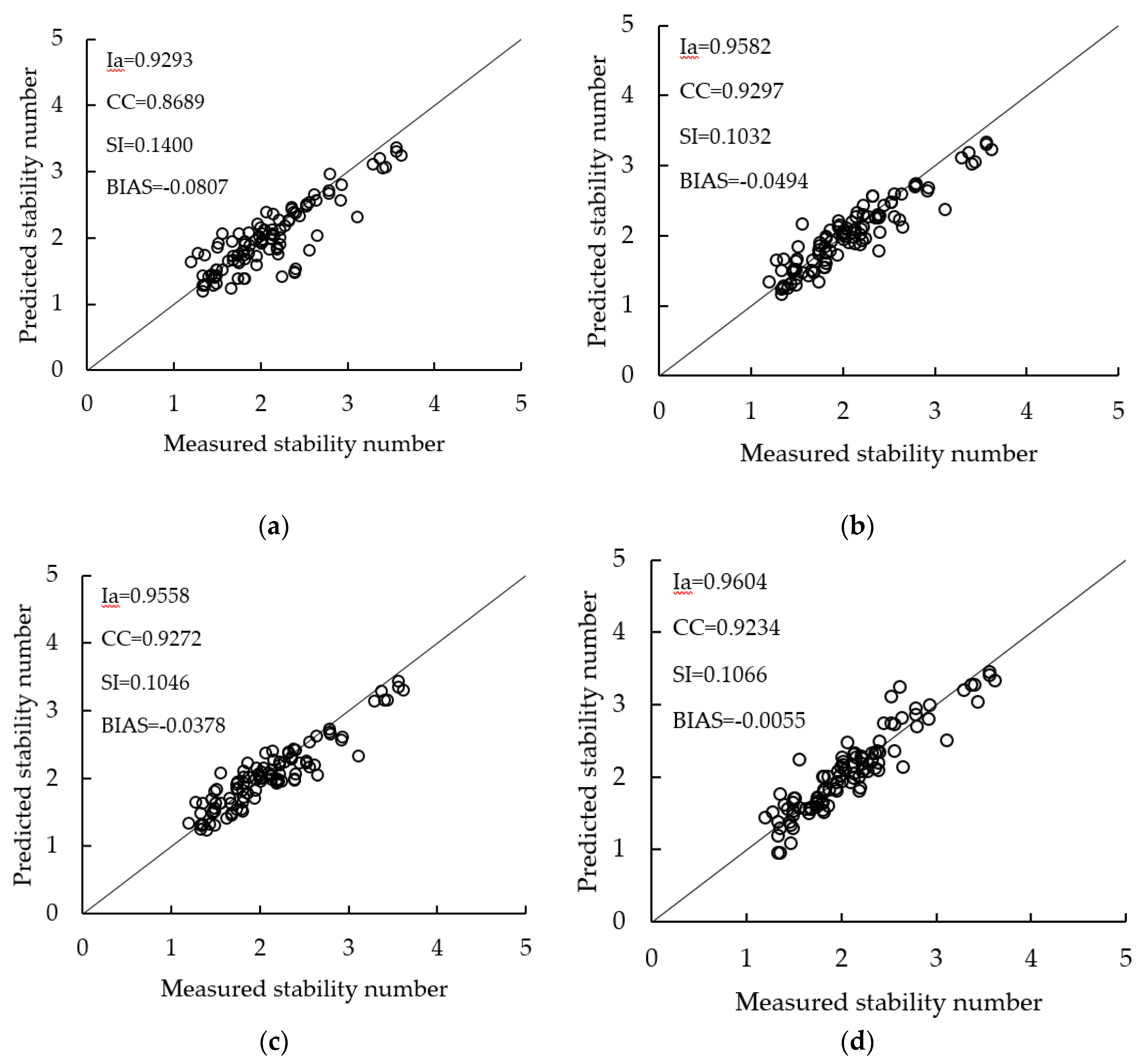
Based on the previous results, the M1 assessment model and the M2 assessment model were built using the ELM algorithm with 45 hidden neurons in the hidden layer and the Sin function as the activation function. The M1 model was used to assess the stability numbers of the breakwater sections at a low damage level (2 ≤ S ≤ 8), and the M2 model was used to assess the stability numbers of the breakwater sections at a high damage level (8 < S < 32). In order to clarify the advantages of the M1 and M2 models, the VM formula [2], the EB formula [8], which was built using the model trees models with a high prediction accuracy, and the GPM1 formula [23], were selected to assess the stability using the same testing data. In the literatures, the EB formula and the GP method have the highest Ia values among those machine learning approaches, which indicates the best prediction performance. The GPM3 formula was not obtained in [23], and the GPM1 model has a similar performance to the GPM3 model presented in [23], so the GPM1 model was selected. These assessment results, predicted by different methods, were prepared and are shown in Figure 5 and Figure 6, respectively.
Figure 5 provides the assessment performance for the breakwater sections that were at a low damage level using the VM formula, EB formula, GPM1 formula and M1 model. As shown in Figure 5, more than half of the predicted stability numbers of the breakwater sections were smaller than the measured values using the VM formula, the EB formula and the GPM1 formula. The assessment performance of the M1 model was more balanced: about half of the predicted stability numbers were smaller than the measured values, while the other half were larger than the measured values.
Several statistical indices were introduced to assess the prediction performance of these approaches, such as the BIAS, CC, SI, and Ia. Lower values of BIAS and SI represent a better assessment performance, and higher values of CC and Ia indicate a better prediction agreement. When the values of CC and Ia are close to 1, this indicates a perfect agreement between the predicted and measured stability numbers. Table 3 lists the statistical index values of the three approaches. As shown in the table, the CC and Ia values of the VM formula are the smallest among these three assessment approaches, while the BIAS and the SI values are the largest, which indicates that the performance of the VM formula has the lowest quality agreement. The CC and Ia values of the EB formula, the GPM1 formula and the M1 model are nearly the same, while on the other hand the SI values of the two methods are also nearly the same. The evaluation indices show that the EB formula, the GPM1 formula and the M1 model have similar abilities for predicting the stability number of breakwaters with a low damage level, but that the M1 model was built based on a smaller size of training data, which indicates that the M1 model has a good generalization ability.
The performance of different approaches was also evaluated for a wider range of damage levels, i.e., 8 < S < 32. The performances of the VM formula, EB formula, GPM1 formula and M2 model are discussed in the following paragraphs. All the predicted results are shown in Figure 6.
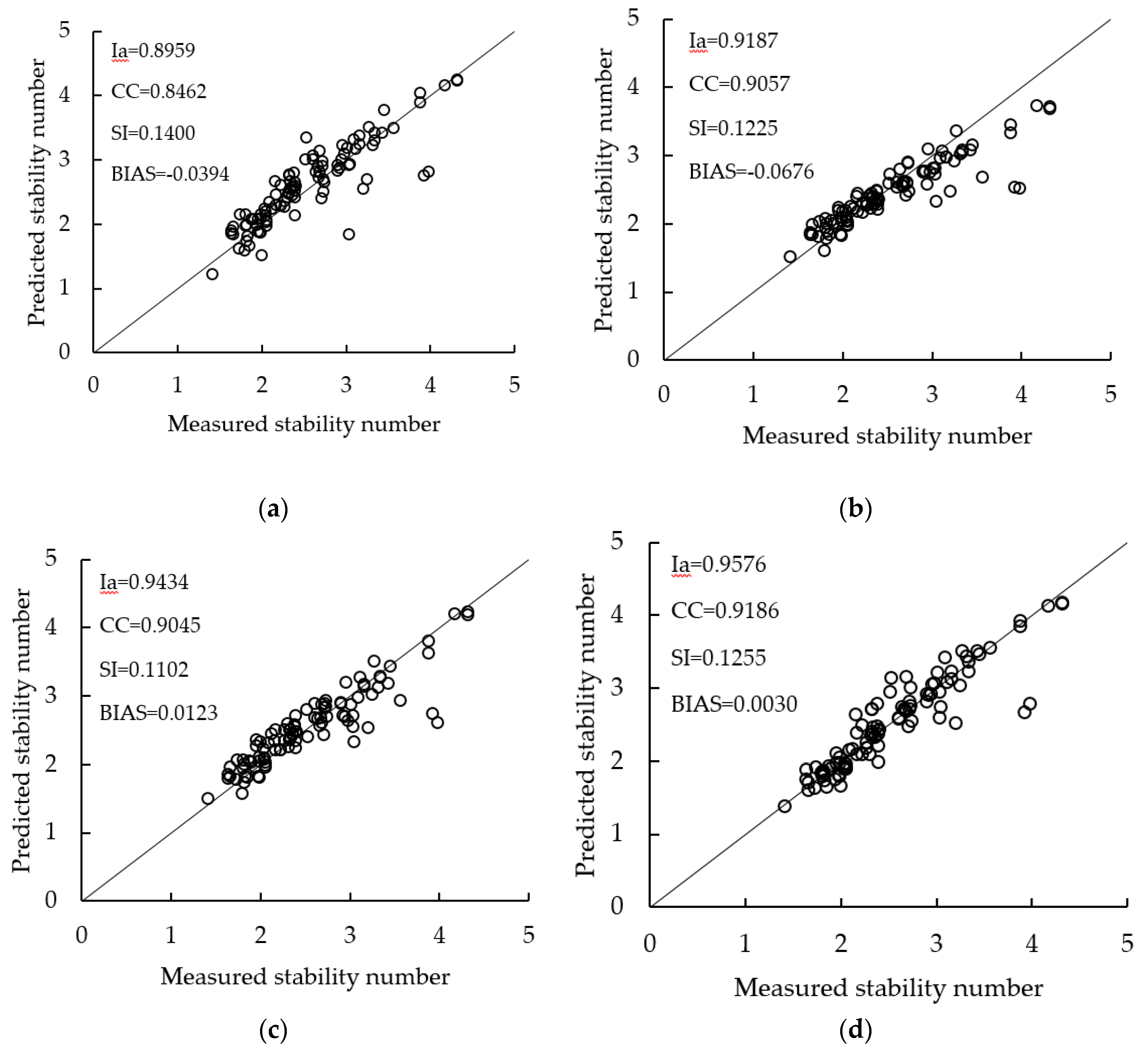
As shown in Figure 6, the VM formula overestimates most of the stability numbers; the same finding could also be found in the study of Etemad-Shahidi and Bali [18]. Meanwhile, on the opposite side, many stability numbers are underestimated by the EB formula. The number of overestimated and underestimated stability numbers is nearly the same for the predictions using the GPM1 model and the M2 model. In addition, the stability numbers predicted by the M2 model are more concentrated on the line of complete agreement than those of the other two approaches. The evaluation indices of these approaches are listed in Table 4. As seen in Table 4, the CC and Ia of the M2 model are the highest, while the BIAS and SI of the M2 model are the lowest, which indicates that the M2 model has the best performance for the stability number prediction of the breakwater sections with a wider damage level range.
Further research was done on the comparison of the assessment performance of different artificial neural network approaches from previous studies. The training parameters and the evaluation indices for these models are listed in Table 5. As can be seen, many kinds of machine learning approaches have been applied in predicting the stability numbers for breakwaters. The number of input parameters of the training models have ranged from 4 to 8, and the number of the training data sets has ranged from 100 to 554. In the current paper, 5 input parameters and 100 sets of training data were used in the training processes of the M1 and M2 models, and the Ia values of the M1 and M2 models are higher than those in many of the previous studies, whose models were built using a larger size of training data and more input parameters. It should also be noted that the Ia or CC values should not be the only evaluation criteria in comparing different methods, since the testing data for each model was not the same. A comparison between the MT2 model (EB formula), GPM1 formula and the ELM method was made in the previous section by using the same testing data, which presented the advantages of the ELM method. The testing data for the MT2 model and the GPM1 formula in [8,23] is not the same testing data used in this paper, which leads to the different Ia and CC values presented in Table 3, Table 4 and Table 5. The CC values of HNN models in the study of Balas, Koç and Tür [13] are slightly higher than the CC values of the M1 and M2 models in the current paper, while the training data is pre-processed by using the principal component analysis (PCA), and the original data sets are 554 sets of experimental data. The PCA could remove the noisy data from the training data and extract the required information [13], so the use of PCA enhances the prediction ability of the machine learning models. It could also be expected that a PCA-ELM model will get a better prediction performance.

4. Conclusions

The aim of the present research was to develop novel and simple Extreme Learning Machine models to predict the stability number for rubble mound breakwater sections. Two ELM models were established to predict the stability number for breakwater sections: the M1 model for low damage levels (2 ≤ S ≤ 8) and the M2 model for high damage levels (8 < S < 32). It was shown that the prediction performances of ELM models were determined by the hidden neurons number, the size of the training data sets and the leaning times; furthermore, the selection of the activation function had little influence on the performance of these models. A comparison of the ELM models and other approaches suggested that the ELM models achieve a good performance with small user-defined parameters and a small training data set size. The key strength of this ELM approach is its good generalization ability and the simple process in establishing the models, which suggested that the ELM models could be an effective and simple tool for breakwater design and stability assessment. In the future, it would be interesting to study the hybrid ELM model, such as the PCA-ELM model, to assess the stability number for rubble mound breakwaters.

Supplementary Materials

The following are available online at https://www.mdpi.com/2077-1312/7/9/312/s1, training data of M1; testing data of M1; training data of M2; testing data of M2.

Author Contributions

Conceptualization, X.W. and Y.L.; methodology and software, X.W.; writing—original draft preparation, X.W., H.L.; writing—review and editing, Y.L., H.L., X.S., S.M. and X.L.; supervision, Y.L.

Funding

This research was funded by the National Natural Science Foundation of China (Grant No. 51520105014), the Postgraduate Research & Practice Innovation Program of Jiangsu Province (Grant No. KYCX19_2328), and the National Key R&D Program of China (Grant No. 2016YFC0402108 & Grant No. 2017YFC0405900).

Acknowledgments

The authors wish to sincerely thank van der Meer for his free database on the stability of rubble mound breakwaters. We also appreciate the reviewers for their valuable suggestions and questions.

Conflicts of Interest

The authors declare no conflict of interest.

Appendix A

Table A1. Weights of M1.
0.5241 26.4975 0.8109−0.42550.6935−0.2008
0.5979 −3.6891 0.88530.67740.6278−0.9448
0.6609 4.1169 0.15180.26820.29910.0216
0.9402 1.1036 −0.55240.75740.7449−0.6862
0.1974 −32.1789 −0.34150.2084−0.7634−0.1137
0.8710 −3.2400 −0.63130.8539−0.32470.9143
0.7430 −29.8057 0.3799−0.2154−0.7326−0.9678
0.2418 5.5068 −0.88440.79030.7482−0.7737
0.5977 −22.8297 0.1486−0.97620.43620.0493
0.7125 1.7637 0.15950.5090−0.99020.1901
0.1448 21.5258 −0.58290.0194−0.7497−0.6622
0.4441 −4.4733 −0.83430.73520.8387−0.2093
0.1918 6.0145 −0.70730.03740.85230.7221
0.7374 52.4679 −0.4033−0.01000.8501−0.7359
0.1496 −9.1100 0.6958−0.28460.9258−0.7403
0.1726 −3.6265 0.4105−0.97110.5676−0.2996
0.8718 −8.6176 −0.9463−0.0608−0.5387−0.6198
0.8638 32.5670 0.71700.0887−0.4715−0.5685
0.2632 13.7757 0.1976−0.0730−0.7203−0.0630
0.1091 −9.6165 0.0072−0.65220.28430.5996
0.3324 3.5370 0.33080.2424−0.64040.6969
BHN1=0.1969InW1=−30.1128InW2=−0.7382−0.5162−0.70290.4078
0.5033 40.9492 −0.1724−0.15710.2812−0.6081
0.7217 −2.1417 0.0027−0.13670.9792−0.1936
0.0935 −4.5602 0.7380−0.41680.7734−0.7967
0.8949 −7.4840 −0.8876−0.75210.75730.1826
0.9296 −51.8195 −0.39700.07880.6631−0.9412
0.3114 −32.1941 0.59910.3968−0.05960.2747
0.8365 0.7267 0.92390.67910.7207−0.1689
0.6055 35.3792 −0.4155−0.4794−0.8263−0.0045
0.1465 5.8143 −0.9828−0.41430.26990.9241
0.9326 −14.1016 0.59110.82710.57720.0635
0.1928 9.7569 −0.4223−0.37000.23380.7443
0.4138 2.4507 −0.1683−0.2665−0.56080.6952
0.0855 −7.5543 −0.9139−0.9217−0.7361−0.3699
0.7125 8.2359 −0.71470.3655−0.7379−0.7774
0.5891 3.9906 0.44420.70300.21630.0113
0.8273 1.0311 0.98520.9763−0.4108−0.4178
0.4677 11.6137 −0.2928−0.8980−0.15450.3437
0.6765 6.5585 0.27510.93460.78670.6949
0.3229 −7.2543 −0.13020.17660.9851−0.9479
0.7244 −8.8476 −0.49260.82060.0350−0.9965
0.1206 −10.8684 0.0382−0.52070.07270.9225
0.5268 −5.1499 −0.1425−0.21910.4494−0.9388
0.2891 8.4672 0.67240.1706−0.46200.9983
Table A2. Weights of M2.
0.4319 −42.0761 −0.9071−0.20110.42720.8116
0.0320 −20.9949 −0.3291−0.0591−0.40200.8705
0.5944 −32.7021 −0.8404−0.60640.88410.6630
0.6627 43.8901 −0.7591−0.24720.81860.9823
0.9264 13.2387 0.8394−0.8762−0.1618−0.3568
0.5949 −20.2892 0.58710.8688−0.09130.7016
0.8525 −63.1985 0.3422−0.7897−0.4640−0.2132
0.8806 −116.6938 0.2035−0.5851−0.2849−0.8588
0.6270 −13.5202 0.78380.9148−0.81210.6147
0.2328 35.2013 −0.1258−0.3481−0.7869−0.1297
0.2941 3.1475 −0.80120.0277−0.4674−0.6218
0.2577 12.4026 −0.8559−0.6591−0.96080.2650
0.6162 0.2601 −0.4507−0.2077−0.49700.7523
0.1584 −3.0225 0.97160.8243−0.44460.6805
0.5654 −7.7516 −0.6291−0.5789−0.52720.3921
0.5730 5.6515 −0.2855−0.53050.43840.8396
0.6728 27.5190 0.02170.4931−0.1090−0.5729
0.7424 0.7453 −0.41980.13800.4327−0.9063
0.7593 36.1610 0.48480.27260.66480.6994
0.7122 44.1426 −0.6639−0.41970.57530.2885
0.6100 −16.2722 −0.0565−0.03940.8366−0.8595
BHN2=0.0537InW2=−1.1557InW2=−0.7270−0.1948−0.1188−0.1234
0.4458 22.3288 0.53870.8696−0.45970.9628
0.8475 −1.6268 0.7513−0.9025−0.66070.6460
0.9733 −83.7627 0.3622−0.6518−0.4596−0.5125
0.8544 22.4302 0.8799−0.2234−0.4083−0.7212
0.3858 −21.6072 −0.53990.19990.1068−0.4392
0.9096 −2.8837 −0.4029−0.62850.8447−0.2820
0.1069 −28.1949 −0.76370.7851−0.3326−0.1881
0.2582 −18.8255 −0.0014−0.11940.58810.2810
0.5765 47.8772 0.5480−0.4075−0.7139−0.6196
0.3990 −5.0568 0.84760.1595−0.46910.1434
0.3779 9.6864 0.7929−0.4492−0.8683−0.4401
0.3411 10.6359 −0.42330.5854−0.92260.3489
0.2897 3.4956 0.8980−0.72440.04540.2533
0.7287 45.6903 −0.45280.58580.1254−0.0241
0.7738 −45.6212 0.8116−0.2095−0.0985−0.6733
0.5252 25.9720 0.2493−0.7998−0.2112−0.3585
0.8545 −50.5003 −0.04410.5296−0.05230.2865
0.0416 3.4476 −0.89480.9645−0.83780.9041
0.6695 8.8539 −0.6859−0.9783−0.8757−0.9541
0.8819 20.7560 0.00100.8347−0.0483−0.2737
0.9352 133.8480 0.2844−0.8046−0.2266−0.8481
0.1300 5.0666 0.6626−0.60740.4537−0.5816
0.9134 14.3699 −0.59420.5127−0.0012−0.3285

Appendix B

The code for the Extreme Learning Machine can be downloaded on the following website: http://www.ntu.edu.sg/home/egbhuang/.

References

  1. Hudson, Y. Laboratory investigation of rubble-mound breakwater. Proc. ASCE 1959, 85, 93–122. [Google Scholar]
  2. Van der Meer, J.W. Rock Slopes and Gravel Beaches under Wave Attack; Delft University of Technology: Delft, The Netherlands, 1988. [Google Scholar]
  3. Pilarczyk, K. Dikes and Revetments Design, Maintenance and Safety Assessment; Routledge: London, UK, 1998. [Google Scholar]
  4. Meulen, T.v.d.; Schiereck, G.J.; d’Angremond, K. Rock toe stability of rubble mound breakwaters. Coast. Eng. 1996, 83, 1971–1984. [Google Scholar]
  5. Kajima, R. A new method of structurally resistive design of very important seawalls against wave action. In Proceedings of the Wave Barriers in Deepwaters, Yokosuka, Japan, 10–14 January 1994; pp. 518–536. [Google Scholar]
  6. Hanzawa, M.; Sato, H.; Takahashi, S.; Shimosako, K.; Takayama, T.; Tanimoto, K. Chapter 130 New Stability Formula for Wave-Dissipating Concrete Blocks Covering Horizontally Composite Breakwaters. In Proceedings of the Coastal Engineering 1996, Orlando, FL, USA, 2–6 September 1996. [Google Scholar]
  7. Vidal, C.; Medina, R.; Lomónaco, P. Wave height parameter for damage description of rubble-mound breakwaters. Coast. Eng. 2006, 53, 711–722. [Google Scholar] [CrossRef]
  8. Etemad-Shahidi, A.; Bonakdar, L. Design of rubble-mound breakwaters using M5′ machine learning method. Appl. Ocean Res. 2009, 31, 197–201. [Google Scholar] [CrossRef]
  9. Van Gent, M.R.A.; Der Werf, I.V. Rock toe stability of rubble mound breakwaters. Coast. Eng. 2014, 83, 166–176. [Google Scholar] [CrossRef]
  10. Thompson, D.M.; Shuttler, R.M. Riprap Design for Wind-Wave Attack, a Laboratory Study in Random Waves; HR Wallingford: Wallingford, UK, 1975. [Google Scholar]
  11. Wei, X.; Lu, Y.; Wang, Z.; Liu, X.; Mo, S. A Machine Learning Approach to Evaluating the Damage Level of Tooth-Shape Spur Dikes. Water 2018, 10, 1680. [Google Scholar] [CrossRef]
  12. Dong, H.K.; Park, W.S. Neural network for design and reliability analysis of rubble mound breakwaters. Ocean Eng. 2005, 32, 1332–1349. [Google Scholar]
  13. Balas, C.E.; Koç, M.L.; Tür, R. Artificial neural networks based on principal component analysis, fuzzy systems and fuzzy neural networks for preliminary design of rubble mound breakwaters. Appl. Ocean Res. 2010, 32, 425–433. [Google Scholar] [CrossRef]
  14. Dong, H.K.; Kim, Y.J.; Dong, S.H. Artificial neural network based breakwater damage estimation considering tidal level variation. Ocean Eng. 2014, 87, 185–190. [Google Scholar]
  15. Kim, D.; Dong, H.K.; Chang, S. Application of probabilistic neural network to design breakwater armor blocks. Ocean Eng. 2008, 35, 294–300. [Google Scholar] [CrossRef]
  16. Erdik, T. Fuzzy logic approach to conventional rubble mound structures design. Expert Syst. Appl. 2009, 36, 4162–4170. [Google Scholar] [CrossRef]
  17. Koç, M.L.; Balas, C.E. Genetic algorithms based logic-driven fuzzy neural networks for stability assessment of rubble-mound breakwaters. Appl. Ocean Res. 2012, 37, 211–219. [Google Scholar] [CrossRef]
  18. Etemad-Shahidi, A.; Bali, M. Stability of rubble-mound breakwater using H 50 wave height parameter. Coast. Eng. 2012, 59, 38–45. [Google Scholar] [CrossRef]
  19. Kim, D.; Dong, H.K.; Chang, S.; Lee, J.J.; Lee, D.H. Stability number prediction for breakwater armor blocks using Support Vector Regression. KSCE J. Civ. Eng. 2011, 15, 225–230. [Google Scholar] [CrossRef]
  20. Narayana, H.; Lokesha; Mandal, S.; Rao, S.; Patil, S.G. Damage level prediction of non-reshaped berm breakwater using genetic algorithm tuned support vector machine. In Proceedings of the Fifth Indian National Conference on Harbour and Ocean Engineering (INCHOE2014), Goa, India, 5–7 February 2014. [Google Scholar]
  21. Harish, N.; Mandal, S.; Rao, S.; Patil, S.G. Particle Swarm Optimization based support vector machine for damage level prediction of non-reshaped berm breakwater. Appl. Soft Comput. J. 2015, 27, 313–321. [Google Scholar] [CrossRef]
  22. Gedik, N. Least Squares Support Vector Mechanics to Predict the Stability Number of Rubble-Mound Breakwaters. Water 2018, 10, 12. [Google Scholar] [CrossRef]
  23. Koc, M.L.; Balas, C.E.; Koc, D.I. Stability assessment of rubble-mound breakwaters using genetic programming. Ocean Eng. 2016, 111, 8–12. [Google Scholar] [CrossRef]
  24. Mase, H.; Sakamoto, M.; Sakai, T. Neural Network for Stability Analysis of Rubble-Mound Breakwaters. J. Waterw. Port Coast. Ocean Eng. ASCE 1995, 121, 294–299. [Google Scholar] [CrossRef]
  25. Wold, S.; Esbensen, K.; Geladi, P. Principal component analysis. Chemom. Intell. Lab. Syst. 1987, 2, 37–52. [Google Scholar] [CrossRef]
  26. Huang, G.B.; Zhu, Q.Y.; Siew, C.K. Extreme learning machine: A new learning scheme of feedforward neural networks. In Proceedings of the IEEE International Joint Conference on Neural Networks, Budapest, Hungary, 25–29 July 2004; Volume 982, pp. 985–990. [Google Scholar]
  27. Rong, H.J.; Ong, Y.S.; Tan, A.H.; Zhu, Z.; Neucom, J. A fast pruned-extreme learning machine for classification problem. Neurocomputing 2008, 72, 359–366. [Google Scholar] [CrossRef]
  28. Huang, G.B.; Ding, X.; Zhou, H. Optimization method based extreme learning machine for classification. Neurocomputing 2010, 74, 155–163. [Google Scholar] [CrossRef]
  29. Pal, M.; Maxwell, A.E.; Warner, T.A. Kernel-based extreme learning machine for remote-sensing image classification. Remote Sens. Lett. 2013, 4, 853–862. [Google Scholar] [CrossRef]
  30. Wei, L.; Chen, C.; Su, H.; Qian, D. Local Binary Patterns and Extreme Learning Machine for Hyperspectral Imagery Classification. IEEE Trans. Geosci. Remote Sens. 2015, 53, 3681–3693. [Google Scholar]
  31. Cheng, L.; Zeng, Z.; Wei, Y.; Tang, H. Ensemble of extreme learning machine for landslide displacement prediction based on time series analysis. Neural Comput. Appl. 2014, 24, 99–107. [Google Scholar]
  32. Abdullah, S.S.; Malek, M.A.; Abdullah, N.S.; Kisi, O.; Yap, K.S. Extreme Learning Machines: A new approach for prediction of reference evapotranspiration. J. Hydrol. 2015, 527, 184–195. [Google Scholar] [CrossRef]
  33. Deo, R.C.; Şahin, M. Application of the extreme learning machine algorithm for the prediction of monthly Effective Drought Index in eastern Australia. Atmos. Res. 2015, 153, 512–525. [Google Scholar] [CrossRef] [Green Version]
  34. Ćojbašić, Ž.; Petković, D.; Shamshirband, S.; Tong, C.W.; Ch, S.; Janković, P.; Dučić, N.; Baralić, J. Surface roughness prediction by extreme learning machine constructed with abrasive water jet. Precis. Eng. 2016, 43, 86–92. [Google Scholar] [CrossRef]
  35. Huang, G.B.; Zhu, Q.Y.; Siew, C.K. Extreme learning machine: Theory and applications. Neurocomputing 2006, 70, 489–501. [Google Scholar] [CrossRef]
  36. Huang, G.; Huang, G.B.; Song, S.; You, K. Trends in extreme learning machines: A review. Neural Netw. 2015, 61, 32–48. [Google Scholar] [CrossRef]
  37. Alexandre, E.; Cuadra, L.; Nietoborge, J.C.; Candilgarcía, G.; Del Pino, M.; Salcedosanz, S. A hybrid genetic algorithm-extreme learning machine approach for accurate significant wave height reconstruction. Ocean Model. 2015, 92, 115–123. [Google Scholar] [CrossRef]
  38. Yin, J.; Wang, N. An online sequential extreme learning machine for tidal prediction based on improved Gath-Geva fuzzy segmentation. Neurocomputing 2015, 174, 243–252. [Google Scholar]
  39. Mulia, I.E.; Asano, T.; Nagayama, A. Real-time forecasting of near-field tsunami waveforms at coastal areas using a regularized extreme learning machine. Coast. Eng. 2016, 109, 1–8. [Google Scholar] [CrossRef]
  40. Imani, M.; Kao, H.C.; Lan, W.H.; Kuo, C.Y. Daily sea level prediction at Chiayi coast, Taiwan using extreme learning machine and relevance vector machine. Glob. Planet. Chang. 2017, 161, S0921818117303715. [Google Scholar] [CrossRef]
  41. Basheer, I.A.; Hajmeer, M. Artifical neural networks: Fundamentals, computing, design, and application. J. Microbiol. Methods 2000, 43, 3–31. [Google Scholar] [CrossRef]
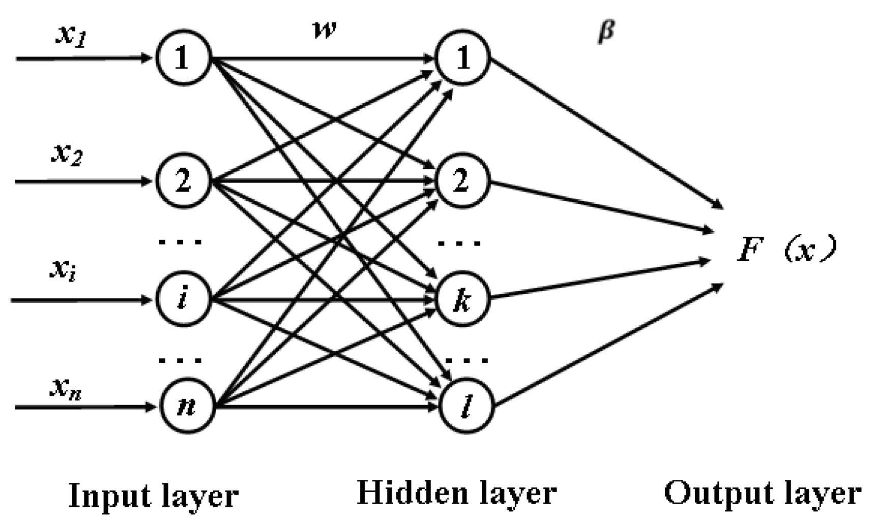
Figure 1. General structure of ELM.
Jmse 07 00312 g001
Figure 2. Parameters used in the M1 and M2 models: (a) the permeability of M1; (b) permeability of M2; (c) damage level of M1; (d) damage level of M2; (e) slope angle of M1; and (f) slope angle of M2.
Jmse 07 00312 g002aJmse 07 00312 g002b
Figure 3. Flow chart of the ELM model establishment.
Jmse 07 00312 g003
Figure 4. Performances of the ELM models with different hidden nodes: (a) Sigmoid function; (b) Sin function; (c) Hardlim function; (d) Tribas function; and (e) Radbas function.
Jmse 07 00312 g004
Figure 5. A performance comparison of different methods: (a) the van der Meer formula; (b) Etemad-Bonakdar formula; (c) GPM1 formula; and (d) M1 model.
Jmse 07 00312 g005
Figure 6. A performance comparison of different methods: (a) the van der Meer formula; (b) Etemad-Bonakdar formula; (c) GPM1 formula; and (d) M2 model.
Jmse 07 00312 g006
Table 1. Various definitions for the damage parameter (damage level).
DefinitionFormulaResearcher
Damage parameter N Δ = A ρ r 9 D 50 ρ α D 50 3 π 6 Thompson and Shuttler (1975) [10]
Damage parameter N 0 = ( H 1 / 3 / Δ D n 1.33 2.32 ) 2 N w 0.5 Hanzawa et al. (1996) [6]
Damage level S = A D 50 3 van der Meer (1988) [2]
Damage level N o d = M B / D n van der Meer (1998) [3]
Damage level S = 0.6 D Kajima (1994) [5]
Note: A is the erosion area in a cross section, ρ r is the bulk density of the material as laid on the slope, ρ a is the mass density of the stone, D 50 is the median diameter of the stone, H1/3 is the average wave height of the Nw/3 highest waves reaching a rubble mound breakwater of a sea state composed of Nw waves, M is the number of stones removed from the structure in a strip, B is the length of the test section, and D is the ratio of the number of displaced units to the total number of units.
Table 2. The range of parameters used in the M1 and M2 models.
ParametersM1 Training DataM1 Testing DataM2 Training DataM2 Testing Data
P0.1, 0.5, 0.60.1, 0.5, 0.60.1, 0.5, 0.60.1, 0.5, 0.6
Sd2–82–88–328–32
cot a1.5–61.5–61.5–61.5–6
Nw1000, 30001000, 30001000, 30001000, 3000
ξm0.67–6.830.67–6.830.7–5.80.7–6.4
Ns1.19–3.611.17–4.621.41–4.31.41–4.3
Table 3. The evaluation indices of the performance of different models (2 ≤ S ≤ 8).
MethodsBIASSICCIa
VM−0.08070.14000.86890.9293
EB−0.04940.10320.92970.9582
GPM1−0.03780.10460.92720.9558
ELM(M1)−0.00550.10660.92340.9604
Table 4. The evaluation indices of the performance of different models (8 < S < 32).
MethodsBIASSICCIa
VM−0.03940.14000.84620.8959
EB−0.06760.12250.90570.9189
GPM10.01230.11020.90450.9434
ELM(M2)0.00300.10220.91860.9576
Table 5. Calculation details of different machine learning approaches.
ResearchersCCIaTraining DataInput ParametersTesting Data
Mase, Sakamoto and Sakai [24]0.91 1006No
Dong and Park [12]I 0.9141006641
II 0.9061005641
III 0.9021006641
IV 0.9151007641
V 0.9521008641
Kim, Dong and Chang [15]I0.9050.9482075119
II0.9130.9542015114
Erdik [16]FL 0.9455796579
Balas, Koç and Tür [13]HNN-10.936 180 (PCA)576
HNN-20.927 180 (PCA)476
Koç and Balas [17]GA-FNN 0.932166 (PCA)542
HGA-FNN 0.947166 (PCA)542
Etemad-Shahidi and Bonakdar [8]MT10.9310.973865193
MT20.9680.9763866193
Koc, Balas and Koc [23]GPM1 0.982077372
GPM2 0.9540722
GPM3 0.9892077372
GPM4 0.99140722
VM 0.969 372
VM 0.65 22
Current StudyELM-M10.9230.9601005100
ELM-M20.9190.9581005100