On the Marine Energy Resources of Mexico

Abstract

The Atlantic and Pacific coasts of Mexico offer a variety of marine energy sources for exploitation. Although the Mexican government has made important efforts to reduce its dependence on fossil fuels, national participation in clean energies is still limited in terms of electricity production. This paper presents a practical theoretical assessment of marine energy sources around Mexico, with the aim of identifying potential zones for subsequent, more detailed, technical evaluations and project implementations. The energy sources considered are ocean currents, waves, salinity, and thermal gradients. Using global databases, the percentages of energy availability for the defined thresholds were computed to establish the prospective regions with the most persistent power availability. This approach proved to offer more meaningful information than simple averaged values. Moreover, some environmental and socio-economic factors to be considered for future ocean energy resource assessments in Mexico were also discussed. The results show that the wave energy potential is highest in the northwest of Mexico (~2–10 kW/m for more than 50% of the time), and that there is a constant source of ocean current energy off Quintana Roo state (~32–215 W/m² for more than 50% of the time). The thermal gradient power is more persistent in the southwest and southeast of the country, where ~100–200 MW can be found 70% of the time. The salinity gradient energy is strongest in the southeast of Mexico. The practical approach presented here can be extended to perform preliminary resources assessments in regions where information is scarce.

1. Introduction

1.1. Motivation

The Mexican government is committed to reducing fossil fuel consumption in the near future; by 2030, 37.7% of the national electricity is expected to come from clean energy sources and by 2050, 50% [1]. The Mexican Centre of Innovation in Ocean Energy (CEMIE-Océano) was thus recently created. This group is made up of academic and industrial institutions, which participate in research and development on the conversion of marine energy sources. Of the many CEMIE-O projects, several are in relatively early technological stages, and some involve evaluating the amount of energy available in Mexico, including its spatial and temporal distribution.

The assessment of available marine energy resources can be theoretical (i.e., gross-averaged energy available), technical (i.e., energy that can be extracted by a particular technology), or practical (i.e., energy that can be extracted considering practical factors, including site restrictions and constraints) [2,3,4].

Often, the theoretical and technical approaches for ocean energy assessment are related to the use of analytical, numerical, and experimental methods to estimate the power potential and identify potential sites for the installation of devices. However, in the practical stage, which must be performed through in-site studies, ecological, economic, and social restrictions often limit the complete evaluation of the resources [4]. In the last decade, research on the estimation of marine resources has greatly increased around the world. Examples of this kind of research include: energy from waves [4,5,6,7,8,9,10,11,12], ocean currents [13,14,15,16], salinity gradients [17,18,19,20], and thermal gradients [21,22,23]. Other works concerned with energy resource assessment for specific countries, such as Korea [24] and Colombia [25], have also been published. This type of preliminary evaluation is important, as it serves as a basis for later, technical studies at specific locations. This paper discusses the theoretical power assessment of ocean energies derived from waves, ocean currents, salinity, and thermal gradients, in Mexican waters.

1.2. Review of Ocean Energy Assessments

1.2.1. Waves

The interaction of winds and the sea surface produces waves, the energy from which is one of the most abundant sources in the world, with the potential to compete with fossil fuels [26,27]. This type of resource can be extracted from the kinetic, or potential, energy of the wave motion [28].

An early estimation of global ocean wave power made by [29] indicated that it was in the order of 1–10 TW. More recently, Sannasiraj and Sundar [7] suggested that the wave energy available worldwide is between 8000–80,000 TW/year and that each wave crest might transmit about 10–15 kW/m.

Some studies, including [5] and [8], have investigated wave power distribution around the world. Cornett [5] analysed global wave energy resources, considering a wave climate prediction of 10 years given by the NWW3-Global wind–wave model (or WAVEWATCH III), which is a tool for simulating ocean behaviour, disregarding shallow water effects. The results of this model were validated from comparisons with data from buoys and satellites available in the literature (e.g., [30]). The results presented by [5] suggest that Mexico has a maximum wave energy potential of 10–20 kW/m, in the Pacific Ocean, specifically. Later, Mork et al. [8] estimated the theoretical global energy potential with the WorldWaves database [31]. This wave data package includes a global offshore wave database, nearshore models for wave propagation (e.g., SWAN) and a statistical analysis module for offshore and nearshore regions. Their results indicate that for Mexico, the lowest power availability is in the Gulf of Mexico and the Gulf of California (~5–10 kW/m), whereas in the northwestern and southwestern regions of the country there is an annual wave power of ~10–20 kW/m, which agrees quite well with the results of [5]. Although the results presented are theoretical, they suggest that potential wave energy in the nearshore regions of Mexico, particularly in sites on the Pacific, could be harvested with appropriate devices. However, temporal variation analyses and well-sustained criteria are still required for pre-selection of potential sites for energy conversion projects.

1.2.2. Ocean Currents

Ocean currents, the continuous flow of ocean water in a specific direction, are attractive as a source of renewable energy due to their predictability, persistence, and sustainability [16]. Some well-known current systems show an almost constant behaviour over time and would be an excellent source of hydrokinetic energy. Many studies concerned with resource characterization in regions near these systems have been published, such as the Agulhas Current near southern Africa [15,32], the Kuroshio current in Asia [33], and the Gulf Stream off the eastern coast of North America [13,14,16].

Marais and Chowdhury [32] considered the upper 200 m of the Agulhas Current along the east coast of South Africa, defining some potential sites and estimating a technical potential of approximately 1200 MW (~3% of the power demand of South Africa in 2010).

Regarding hydrokinetic power evaluation in North America, Duerr and Dhanak [13] investigated a section of the Florida Current of the Gulf Stream. The evaluation was made with databases available (e.g., the HYbrid Coordinate Ocean Model, HYCOM, and Acoustic Doppler Current Profilers, ADCPs), suggesting a total power availability of 20–25 GW. However, estimated more realistically, the power was much less—1–4 GW. In their estimation, they also considered technical evaluations, including turbine arrays, concluding that these might yield ~200 MW. Some years later, Yang et al. [16] generated a geodatabase for the ocean current power available in USA, highlighting the Gulf Stream system. They stated that there could be a kinetic power density in that region (i.e., power per unit area) of over 2 kW/m², while in other regions of the USA, power extraction was probably less than 100 W/m². In the same year, Kabir et al. [14] evaluated the available power of the Gulf Stream at a higher latitude, in the North Carolina region. They considered current variability and found a power density of between 0.5 and 1 kW/m². These results suggest that there could also be opportunities for hydrokinetic energy extraction off Mexico, where the Gulf Stream has an almost constant flow from the Caribbean Sea.

1.2.3. Thermal Gradients

Thermal gradient energy is generated from the heat interchange between fluids at different temperatures. The first demonstration of thermal gradient energy conversion [34] was an OTEC (Ocean Thermal Energy Conversion) plant installed in Matanzas Bay, Cuba in 1929 by Georges Claude. It was a 2 km-long plant, with pipes 1.6 m diameter, which failed due to the selection of a poor site and problems with the power and seawater systems. Despite a second failure in 1930, Georges Claude’s plant did generate ~22 kW of electric power for 10 days, using a temperature gradient of 14 °C [34].

Much later, OTEC prototypes in Hawaii in 1979 (~50 kW of gross power), Tokyo in 1981 (~120 kW of gross power), and again in Hawaii in 2015 (~100 kW of power capacity) have continued the development of thermal gradient energy technology. The 2015 plant was the first closed-cycle onshore plant. Installed by Makai Ocean Engineering, it was one of the largest OTEC power plants in the world [35].

A reliable global thermal gradient resource estimation is difficult to attain due to several logistic and technical constraints. Gross estimates are between 5 TW and 1000 TW [35]. However, it is important to consider that thermal gradient power estimation can also depend on the type of plant deployed, as well as the available thermal gradient through time.

OTEC plants can be closed-cycle (CC-OTEC), open-cycle (OC-OTEC), or hybrid-cycle (HC-OTEC) systems [27]. The former employ a working fluid to flow between two heat exchangers in a closed-cycle. The second consider low pressure steam as the working fluid. The electric power is generated from the steam in a generator. Then, cold water from deep in the ocean is used to condense the steam. The hybrid-cycle systems combine the procedures of the closed- and open- cycle systems. Thus, as can be inferred, the evaluation of thermal gradient energy resources depends a great deal on the characteristics of the plant considered.

It has been suggested that OTEC may offer higher power availability compared to other types of ocean energies, at around ~14 TW [36]. In tropical areas, it is estimated that OTEC systems could offer about 1000 TW [37]. Nihous [38] proposed a widely used formulation for the gross and net power estimations associated with a thermal energy gradient. Some years later, Nihous [39] extended this approach to perform a preliminary assessment of potential ocean thermal energy worldwide using the available databases. Evaluations of thermal gradient energy resources have also been performed in specific regions, such as Puerto Rico [40], Florida [35], the Hawaiian Islands [41], parts of the Indian Ocean [42], and Southeast Asia [43].

For Mexico, an estimate of thermal energy resources in specific regions was recently undertaken by [22], who found that several sites on the coasts of Mexico are suitable for the installation of OTEC plants. However, these authors did not examine the whole country and concluded that temporal variations in thermal gradients still have to be considered when selecting suitable sites for device deployment. So, an evaluation of thermal gradient energy availability for all of Mexico is still needed.

1.2.4. Salinity Gradients

Salinity gradient energy (SGE) is also known as “blue energy” or “osmotic power” [44], and comes from the interaction of a fluid of low salinity concentration, such as river water, with a fluid of higher salinity, such as seawater. The energy resulting from this phenomenon can be converted into electric power by appropriate conversion devices. SGE can be harnessed where there is a considerable difference between the salinities of the two fluids, either in a lake–river system (i.e., the rivers have their mouths in a lake, as in [18]) or in an ocean–river system (i.e., the rivers have their mouths in an ocean, as in [45]).

The SGE process can be better understood as a reverse desalination process. In a desalination process, energy is necessary for the extraction of freshwater from seawater [46], so a reverse desalination process would release energy.

Since the 1950s, SGE has been seen as a widely available alternative source of electrical power, as reported by [47], who proposed the process of reverse electrodialysis, explaining that the energy produced from mixing a river and seawater would be similar to that delivered by a waterfall ~270 m high. Although there were several studies on SGE in the 1970s and 1980s, a practical application was not possible at that time, due to a lack of technology [19]. Recent advances in membrane technology have now made SGE a feasible source of energy.

Early estimations of theoretical SGE resources in the world ([48,49]) suggested that the global SGE potential is between 1.4 and 2.6 TW, that is, between 40–80% of the current power demand [19]. More recent global SGE estimations have been made by [50] and [51], who reported SGE potentials of 0.228 TW and 3.13 TW, respectively. Alvarez-Silva and Osorio [45] recently reported that the global estimation of theoretical SGE is 0.22–3.16 TW.

More recently, Alvarez-Silva et al. [17] made a global assessment of SGE extraction at river mouths. They considered that the theoretical potential is affected by constraints related to the suitability, sustainability, and reliability of SGE exploitation and included these constraints in their power estimation. An extraction factor, a capacity factor, an adequate selection of sites, and the assumptions made in the models used to estimate the theoretical potential have to be considered in the final estimation of power. Taking these factors into consideration, they concluded that a more realistic global potential would be ~625 TWh per year (i.e., ~0.071 TW), which is approximately 3% of the global electricity consumption.

As Mexico is one of the countries with the most ocean–river systems in the world [17], this suggests SGE generation will be possible in many zones where rivers interact with seawater. However, to the best of the authors’ knowledge, there is no theoretical resource assessment of this type of ocean energy for Mexico.

1.3. Objectives

While ocean energy is not available for all countries, three quarters of the world’s nations have coastlines and therefore could benefit in some way from their ocean energy resources. This is the case for Mexico, which has energy resources in the Atlantic and the Pacific Oceans. Since there is no documented resource assessment of the different types of ocean energies for Mexico, the main objective of this paper is to theoretically evaluate the available power from waves, ocean currents, thermal gradient, and salinity gradient as the path to facilitate the selection of sites, where further in depth studies should be carried out. Power availability is presented as thresholds of minimum power; this may help in the selection of energy conversion devices. A statistical analysis is performed to determine monthly power availability and variability at prospective locations for each source of marine energy. Moreover, some environmental, economic, and social factors to consider in future marine energy projects in Mexico are also discussed.

The present study is organised as follows: the theoretical methods for power estimation and the data used for each type of ocean energy are described in Section 2 and Section 3, respectively. The main results of the theoretical power available for each type of energy are presented in Section 4, describing the regions where potential power is more persistent. Section 5 shows a monthly-variability analysis for particular locations, and Section 6 presents relevant environmental, economic, and social factors to be considered in Mexican MRE (Marine Renewable Energy) projects. Finally, the main conclusions and possibilities for future work are summarised in Section 7.

2. Theoretical Approaches to Marine Energy Power Estimation

The theoretical potential of any type of ocean energy source is the physical maximum of usable energy in a particular region in a specific period of time [51]. In practice, only part of the theoretical potential can actually be extracted due to ecological, technical, and economic constraints. This section briefly describes the engineering methods employed to estimate the available theoretical (gross) power of the ocean energies considered in this paper. Only the most important equations have been given here, as details for each model can be found in the references given. It should be noted that the units of theoretical power vary for each approach.

2.1. Wave Power

Considering linear wave theory in deep waters, the theoretical power that can be extracted from ocean waves (P_OW, in W/m) can be estimated by [52,53]:

$${\mathrm{P}}_{\mathrm{OW}}=\frac{{\mathrm{W}\mathsf{\rho }\mathrm{g}}^2{\mathrm{T}}_{01}{\mathrm{H}}_{\mathrm{s}}^2}{64\mathsf{\pi }},$$

(1)

where W is the wavefront (assumed to be 1 m), $\mathsf{\rho }$ is seawater density (1025 kg/m³), H_s (in m) is the significant wave height or the average height, and T₀₁ (in s) is its corresponding energy period.

2.2. Ocean Current Power

The theoretical gross power of ocean currents (P_OC, in W/m²) is considered as the power generated by a fluid stream across a unitary cross-section [14,15]:

$${\mathrm{P}}_{\mathrm{OC}}=\frac{1}{2}{\mathsf{\rho }\mathrm{V}}^3,$$

(2)

where V is the water stream velocity (in m/s). In this work, V was considered as the resultant velocity from the northward and eastward velocity components, available in the databases used (see Section 3). It is important to mention that such an approach disregards velocity variations, which might give underestimations of power [14], but it is sufficient for preliminary estimation purposes.

2.3. Thermal Gradient Power

The empirical approach to calculate the gross electrical power of an OTEC plant proposed by Nihous [39] (P_TG, in W) was used in this work:

$${\mathrm{P}}_{\mathrm{TG}}=\frac{3{\mathsf{\rho }\mathrm{c}}_{\mathrm{p}}{\mathrm{Q}}_{\mathrm{ww}}\Delta {\mathrm{T}}^2\mathrm{E}}{16{\mathrm{T}}_{\mathrm{s}}\left(1+{\mathrm{Q}}_{\mathrm{ww}}/{\mathrm{Q}}_{\mathrm{cw}}\right)},$$

(3)

where $\mathsf{\rho }$ is seawater density (1025 kg/m³) and c_p is the specific heat of the seawater (~4000 J/kg°K, [39]). $\Delta \mathrm{T}$ (in °K) is considered here as the temperature difference between the sea surface and 1000 m water depth and Ts (in °K) is the temperature at the sea surface. ${\mathrm{Q}}_{\mathrm{ww}}$ (in m³/s) is defined as the OTEC warm (surface) sea water volume flow rate and ${\mathrm{Q}}_{\mathrm{cw}}$ (in m³/s) as the cold (1000 m-depth) water volume flow rate. The following assumption was made on these parameters: given that the extractable thermal gradient power depends on the capacity of the OTEC plant to maintain adequate flow rates, a typical 100 MW OTEC plant was considered, for which the seawater flow rate Q_cw was assumed to be 250 m³/s [2]. On the other hand, Q_ww was considered equal to 1.6 Q_cw, as in the study performed by [39]. Finally, in Equation (3), E is the efficiency of a turbogenerator. However, as this is a theoretical assessment, disregarding local and friction energy losses, this parameter was considered equal to 1. For a more technical assessment of available OTEC, the reader is referred to [36,39], where the method is presented more fully.

2.4. Salinity Gradient Power

Theoretically, energy can be released by reversing any desalination process [46]. The mechanism of mixing salt solutions of different concentrations under constant pressure and temperature conditions is described in the Gibbs free energy of mixing, which is commonly used to estimate the extractable energy from such an interaction [20,46]. Details of this method can be found in [17,18,46], among others.

Following [19], the amount of electric power generated by the interaction between a river and a fluid of higher salinity concentration (i.e., seawater), depends on several factors. These include the volumes of water involved, the differences in temperature between them, the chemical characteristics of the salt, environmental restrictions, available infrastructure, and the demand for electricity. Although a complete assessment of the available salinity gradient power would depend on these factors, for preliminary purposes it is possible to perform a theoretical estimation with only four variables [18,19]: temperature, river salinity, sea salinity, and discharge at the river mouth. In this framework, the theoretical potential of energy produced by a salinity gradient (P_SG, in kW) in a river–ocean system is estimated by the practical approach proposed by [54], which was also used by [19] and [18]:

$${\mathrm{P}}_{\mathrm{SG}}=2{\mathrm{Q}}_{\mathrm{riv}}{\mathrm{RT}}_{\mathrm{mouth}}\left({\mathrm{S}}_{\mathrm{riv}}\ln \frac{2{\mathrm{S}}_{\mathrm{riv}}}{{\mathrm{S}}_{\mathrm{riv}}+{\mathrm{S}}_{\mathrm{sea}}}+{\mathrm{S}}_{\mathrm{sea}}\ln \frac{2{\mathrm{S}}_{\mathrm{sea}}}{{\mathrm{S}}_{\mathrm{riv}}+{\mathrm{S}}_{\mathrm{sea}}}\right),$$

(4)

where Q_riv is the river discharge (in m³/s), R is a universal gas constant equal to 8.314 J/mol°K [18], and T_mouth (in °K) is the water temperature at the river mouth where it meets the ocean. S_riv and S_sea are the river and seawater salinities (in mol/L), respectively. For practical purposes, following [54] and [19], given that there is a lack of available data for Mexican rivers, the river salinity (S_riv) is considered a constant 0.005 mol/L. The seawater salinities were obtained from databases in gr/kg units (Section 3). Then, to convert them to mol/L units, their salinity concentrations due to NaCl were taken as 58.4 gr/mol.

It is important to mention that all the parameters used to estimate the theoretical potential vary with time, so a practical alternative for calculating the P_SG is to employ average values [18]. Thus, annual averaged river discharges (Q_riv), as well as sea salinities and temperatures near rivers mouths in the ocean (S_sea and T_mouth, respectively), were obtained from the data sources described in Section 3.

3. Data Sources

In the present study, databases of simulated and measured variables were used for the theoretical models described in Section 2 for each ocean energy source. First, data for the estimation of the wave energy potential was obtained from the ERA-Interim public dataset, which is one of the latest and most complete global atmospheric reanalyses and is produced by the European Center for Medium-Range Weather Forecasts (http://apps.ecmwf.int/datasets/data/interim-full-daily/levtype=sfc/). Details of the reanalysis methods used to obtain the data are fully described in [55]. Significant wave heights (H_s) and their correspondent energy periods (T₀₁) were extracted from the ERA-Interim reanalysis, considering daily data from 1 September 2008 to 31 August 2018 for practical purposes, with a spatial resolution of 1/8° × 1/8°.

The input data for analysing the theoretical power due to ocean currents (i.e., northward and eastward water velocities), thermal gradients (i.e., temperatures at different water depths) and salinity gradients (i.e., temperatures and salinities close to river mouths), were taken from the HYCOM ocean model databases (https://hycom.org/data/glbu0pt08/expt-91pt2). This model is a data-assimilative hybrid isopycnal-sigma-pressure coordinate ocean model (more details in [56]). The data from the HYCOM+NCODA Global Analysis (GLBu0.08/expt_91.2), obtained at a temporal resolution of one day and a spatial resolution of 1/12° × 1/12°, were employed. The daily hindcasting data used was from 1 September 2013 to 31 August 2018. This database was selected due to the higher spatial resolution compared to other databases [13].

Finally, for salinity gradient power estimation, the river discharge data for Mexican rivers was obtained from the global database of SAGE (Center of Sustainability and the Global Environment), University of Wisconsin–Madison (http://nelson.wisc.edu/sage/data-and-models/riverdata/), which provides measurements from 3681 stations situated in the most important rivers in the world. Data for 18 river mouths in the Pacific and 11 river mouths in the Atlantic were used and the period of data acquisition for each station varied. That is, for each river, monthly averages for different years were reported in the database. Then, with the monthly averages, annual average values for the corresponding years were given (see the database for specific details for each river). These annual averages were employed in the analyses. However, it is important to bear in mind that the annual discharge data provided may not be the most recent data and the gauging stations were not located at river mouths in all cases. Regardless of these limitations, the data were deemed to be suitable for this work.

4. Theoretical Power of Marine Energy Sources

This section gives the estimations of theoretical power and the identification of potential regions for energy extraction. The results for energy from waves, ocean currents, and thermal gradients are presented in Section 4.1, Section 4.2 and Section 4.3, respectively. For these sources, the theoretical power was estimated as the availability percentage, for the five-year period, of specific thresholds; namely 2, 5, 10, and 15 kW/m for wave energy; 32, 176, 512, and 1730 W/m² for current energy; and 100, 150, 200, and 250 MW for thermal gradient energy. In other words, the results are the percentage of days for which the available power was equal to, or higher than, the thresholds (see Figure 1, Figure 2 and Figure 3).

Table 1. Maximum power availability (in percentage of days over the ten-year period considered) for the energy from waves, currents, and thermal gradients.

State	Waves	Currents	Thermal Gradients
	>2/>5/>10/>15 kW/m	>32/>176/>512/>1730 W/m2	>100/>150/>200/>250 MW
	(%)
1-Baja California Sur	90–100/90–100/80–90/70–80	50–60/0–10/0–10/0–10	90–100/90–100/50–60/30–40
2-Baja California	90–100/90–100/80–90/70–80	30–40/0–10/0–10/0–10	90–100 */40–50 */0–10 */0–10
3-Sonora	0–10/0–10/0–10/0–10	50–60 */0–10/0–10/0–10	90–100 */70–80 */40–50 */30–40
4-Sinaloa	90–100/80–90/40–50 */20–30 *	20–30 */0–10/0–10/0–10	90–100 */90–100 */50–60 */30–40
5-Nayarit	90–100/80–90 */40–50 */20–30 *	20–30 */0–10/0–10/0–10	90–100 */90–100 */60–70 */60–70
6-Jalisco	90–100/90–100/60–70/60–70	20–30/0–10/0–10/0–10	90–100/90–100/70–80/60–70
7-Colima	90–100/90–100/60–70/60–70	20–30/0–10/0–10/0–10	90–100/90–100/80–90/70–80
8-Michoacán	90–100/90–100/60–70/60–70	20–30/0–10/0–10/0–10	90–100/90–100/80–90/70–80
9-Guerrero	90–100/90–100/60–70/60–70	30–40/0–10/0–10/0–10	90–100/90–100/90–100/80–90
10-Oaxaca	90–100/90–100/60–70/60–70	70–80/0–40/0–10/0–10	90–100/90–100/90–100/80–90
11-Chiapas	90–100/90–100/60–70/60–70 *	50–60 */0–30 */0–10/0–10	90–100 */90–100 */90–100 */60–70 *
12-Quintana Roo	60–70/60–70 */10–20/10–20 *	90–100/90–100/60–70/10–20	90–100/90–100/90–100/90–100
13-Yucatán	40–50/40–50/10–20/10–20 *	20–30 */0–10/0–10/0–10	-
14-Campeche	20–30/10–20/10–20 */10–20	0–10/0–10/0–10/0–10	-
15-Tabasco	30–40/30–40/20–30/10–20	20–30/0–10/0–10/0–10	-
16-Veracruz	50–60/40–50/30–40/10–20	50–60/0–20/0–10/0–10	90–100 */90–100 */90–100 */40–60 *
17-Tamaulipas	60–70/60–70 */30–40/10–20	40–50/0–20/0–10/0–10	90–100 */90–100 */90–100 */60–70 *

* =Regions located farther from the coast.

summarises the information of these figures for all the coastal states of Mexico. In Table 1, the percentages of power availability for waves, currents, and thermal gradients are expressed in terms of the ranges presented in the corresponding figures. For instance, for the case of the power availability from waves in Baja California Sur, the ranges 90–100, 90–100, 56–60, and 30–40 that are shown in the table correspond the percentage ranges at which the available power surpasses the thresholds of 2, 5, 10, and 15 kW/m², respectively.

Section 4.4 shows the results for the theoretical power from salinity gradient energy. Unlike the other energy sources, these results were examined using the available river discharge data. That is, the theoretical potential was examined in terms of mean and standard deviation values, considering the annual averaged river discharges of the database.

It is important to mention that, while the theoretical ocean energy potential for some Mexican islands is included in the results, it was not analysed due to limitations of infrastructure at these sites. Moreover, in the analyses of waves, currents, and thermal gradient energies, the data were analysed for a distance of ~100 km from the coast, in line with the maximum length of a DC power cable, as explained by [57]. This distance was set for the preliminary evaluation of resources, as the authors believe that initial MRE projects in Mexico might begin near to available infrastructure and close to the coast. To generate Figure 1, Figure 2 and Figure 3, a total of 144,789 nodes from databases, covering Mexican territorial waters, were considered for the analyses. From the nodes database, interpolation was performed to generate rasters (with a spatial resolution of 0.09 and 0.09 degrees), and subsequently polygon shapefiles, covering all of the Mexican coastal zones.

4.1. Wave Energy Results

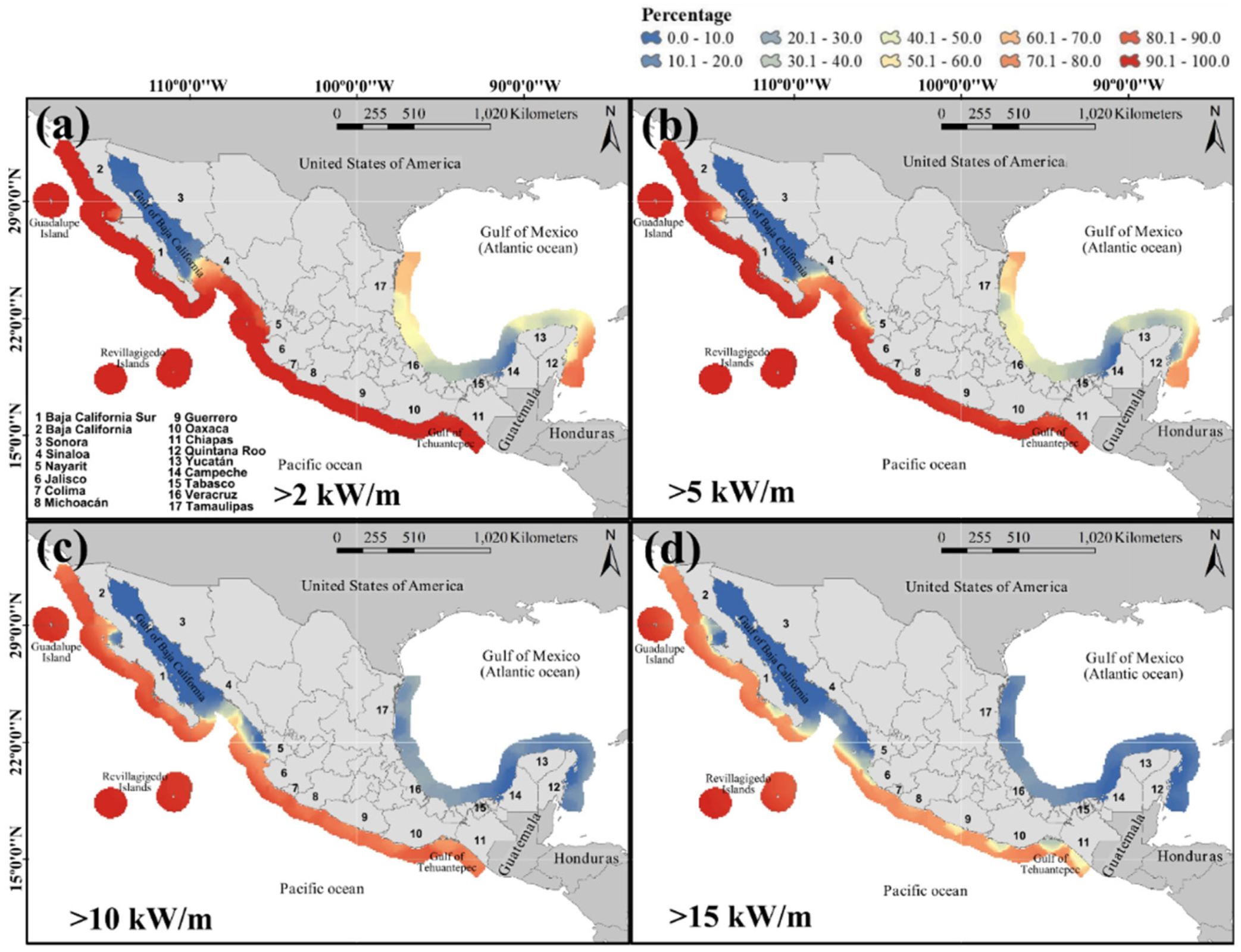
Figure 1 shows the theoretically available wave power as percentages of the days throughout the ten-year period. To better represent this power availability, four power thresholds were used to identify the regions with the most, and most persistent, power potentials. Figure 1a–d shows the regions where wave power is equal to, or greater than, 2, 5, 10, and 15 kW/m, respectively. The first threshold, 2 kW/m, was defined from the power matrices of wave energy converters described elsewhere [58]. These data suggest suitable operating conditions for devices are significant wave heights H_s > ~1 m and associated energy period T₀₁ > ~5 s.

Figure 1a–d shows that the Mexican Pacific coasts have the highest, most persistent power availability, while the Atlantic coasts have lower energy potential and are more susceptible to variations. Figure 1a,b and Table 1 show that it would be possible to extract power of ~2–5 kW/m almost all the time (~90–100%) in at least eight states on the Pacific coast (states 1, 2, 6–11). Power in the range of 5–10 kW/m and 10–15 kW/m could be extracted in these regions ~50–100% of the time (Figure 1b,c) and ~30–50% of the time (Figure 1c,d), respectively. In the Atlantic states 12, 13, 15, 16, and 17, (Figure 1a), wave power in the range of ~2–5 kW/m could be obtained only about 20–50% of the time.

Overall, the results suggest that wave energy extraction would be possible along the western coasts of Mexico, with available power of up to ~10 kW/m, for at least 50% of the time. These results are in good agreement with the descriptions of [5] and [8], who published maps showing a possible annual wave power of ~10–20 kW/m here. These comparisons were made with global estimations since, to the authors knowledge, specific studies for Mexico including details of power near coastal regions have not been made. A very preliminary estimation can be found in [59].

4.2. Current Energy Results

The results for the ranges of operation, defined by the minimum and maximum (cut-in and cut-off) operational flow velocities of typical hydrokinetic devices, are presented in Figure 2.

Typical cut-in velocities of marine turbines range between 0.5 and 1.0 m/s [15,60]. However, there are hydrokinetic devices, such as the VIVACE (Vortex Induced Vibrations for Aquatic Clean Energy) system, that take advantage of the VIV (Vortex Induced Vibrations) generated in oscillating cylinders, which have a cut-in velocity of about 0.4 m/s [3]. Unlike wind turbines, which can operate at a wind speed of ~11–13 m/s, the free stream velocity for hydrokinetic turbines is about 3 m/s [61,62]. Higher velocities may damage the blades and cause failure [63]. Therefore, to analyse the availability of ocean current energy resources, results were evaluated from a minimum power threshold (~32 W/m²), considering a cut-in flow velocity of 0.4 m/s.

For the analyses, velocities at the free surface were considered, since in the first 100 m of water depth they are highest. It has been reported that there is no significant variation in water velocities in the first 50 m of depth, so this seems to be where hydrokinetic devices should be deployed [14].

Figure 2 shows the percentages of days in the five-year period when power availability from currents was over 32 (Figure 2a), 176 (Figure 2b), 512 (Figure 2c), and 1730 (Figure 2d) W/m², obtained with current velocities of ~0.4, ~0.7, ~1.0, and ~1.5 m/s, respectively. In Figure 2a, it can be seen that the regions with more than this minimum flow velocity included areas in the Gulf of Baja California (states 1–4), the Gulf of Tehuantepec (states 9–11), and the Gulf of Mexico (states 12, 16, 17). This means that it is possible to obtain more than 32 W/m² for more than 50% of the time considered. However, Figure 2b,c shows that persistent power of over 176 W/m² and 512 W/m², respectively, is available more than 50% of the time in the waters off Quintana Roo, the Gulf Stream. Figure 2d shows that in no area of Mexico is current energy of over 1730 W/m² available.

The results presented in Figure 2 and Table 1 suggest that it is possible to extract energy for low current hydrokinetic devices for about 50% of the time in some regions; off Baja California Sur, Baja California, Sonora, Sinaloa, Michoacán, Oaxaca, Quintana Roo, Yucatán, Veracruz, and Tamaulipas. However, it can be seen that the state of Quintana Roo is where the highest levels and almost permanent energy extraction would be possible. It is also important to mention that the Gulf of Baja California has the potential for harvesting energy from tidal currents, as demonstrated by [64], who performed a detailed analysis of this area.

4.3. Thermal Gradient Energy Results

Vega [65] recommended that the most cost-effective OTEC plants be deployed where there is deep water close to shore. This seems to be a good strategy for initial OTEC projects in emerging countries, such as Mexico. The available thermal energy resources were analysed, taking into consideration a water depth of at least 1000 m and a distance from the shore of less than 100 km. The percentages of time over the five-year period at which power of over 100 MW, 150 MW, 200 MW, and 250 MW was available are shown in Figure 3a–d, respectively.

The results indicate that there is a persistent (90–100%) power availability of 100–150 MW in the waters off states 1, 4–10, 12, 16, and 17 (Figure 3a,b, Table 1). Within these areas, there are places where a water depth of 1000 m is close to the coast and therefore these areas are attractive for thermal energy extraction: close to states 1, 6–10, and 12. In fact, these areas have ~150–200 MW available power more than 70% of the time (Figure 3b,c, Table 1). These regions also have ~200–250 MW of power more than 60% of the time.

Overall, the results suggest that the best locations in Mexico to extract thermal gradient energy are off Colima (7), Michoacán (8), Guerrero (9), Oaxaca (10), and Quintana Roo (12). On the other hand, plants of a lower capacity (100–150 MW) could be deployed in specific locations off Baja California Sur (1), Sinaloa (4), Nayarit (5), Veracruz (16), and Tamaulipas (17), where there is almost constant availability of resources, farther from the coast.

4.4. Salinity Gradient Energy Results

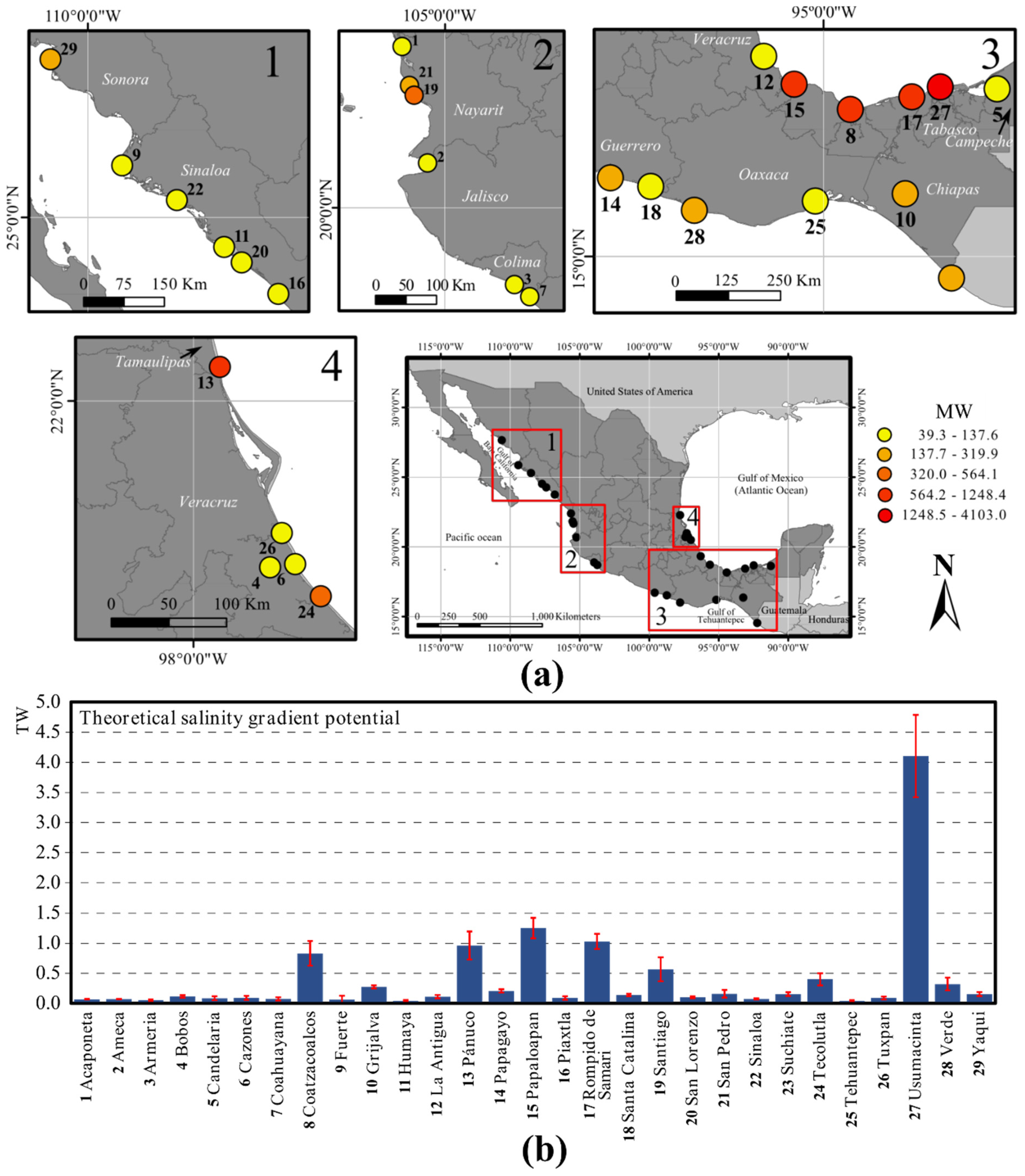
The theoretical power available from salinity gradients, in terms of mean and standard deviation values, is presented in Figure 4. Figure 4a shows the location of the river stations and the available salinity gradient power (in MW). Five power intervals were established, considering mean power values, to classify the resource availability for each river. Figure 4b presents the mean and standard deviation values of power (in TW) for each location.

The river Usumacinta (N°27, Figure 4a) had the highest potential power generation capacity of all the rivers analysed, with 4.10 ± 0.68 GW. This agrees quite well with the theoretical potential of 3.6 GW reported by Alvarez-Silva et al. [17], who used the Gibbs approach for their estimation. The river mouths with the highest salinity gradient power availability were on the Gulf of Mexico, especially in Tamaulipas (N°13, 958.55 ± 232.7 MW), Veracruz ((N°8, N°15), (828.58 ± 204.9 MW, 1248.48 ± 169.7)) and Tabasco (N°17, 1026.91 ± 126.1 MW). On the Pacific coast, Nayarit had the highest potential (N°19, 564.5 ± 199 MW). From these results, it would seem that there is a substantial potential for salinity gradient energy in Mexico, particularly in the rivers mouths on the Gulf of Mexico, in the southeast of the country, which is one of the most humid tropical environments in Mexico.

Despite the limitations of this analysis, including the approximation of estimations due to the differences in the databases for the time periods of the sampling, the disregarding of temporal discharge fluctuations, and the simplified theoretical approach, it is useful as a preliminary tool to identify regions where there is salinity gradient energy potential. Further research is required to evaluate the most appropriate places, implementing more specific technical evaluations of the salinity gradients.

5. Monthly Variations of Theoretical Power at Specific Locations

This section presents an analysis of the monthly variability of the theoretical power found at some of the locations with maximum power availability from waves, currents, and thermal gradient, as detailed in the previous section (see Table 1). An analysis for salinity gradient was not performed, due to the lack of discharge data over time in the databases.

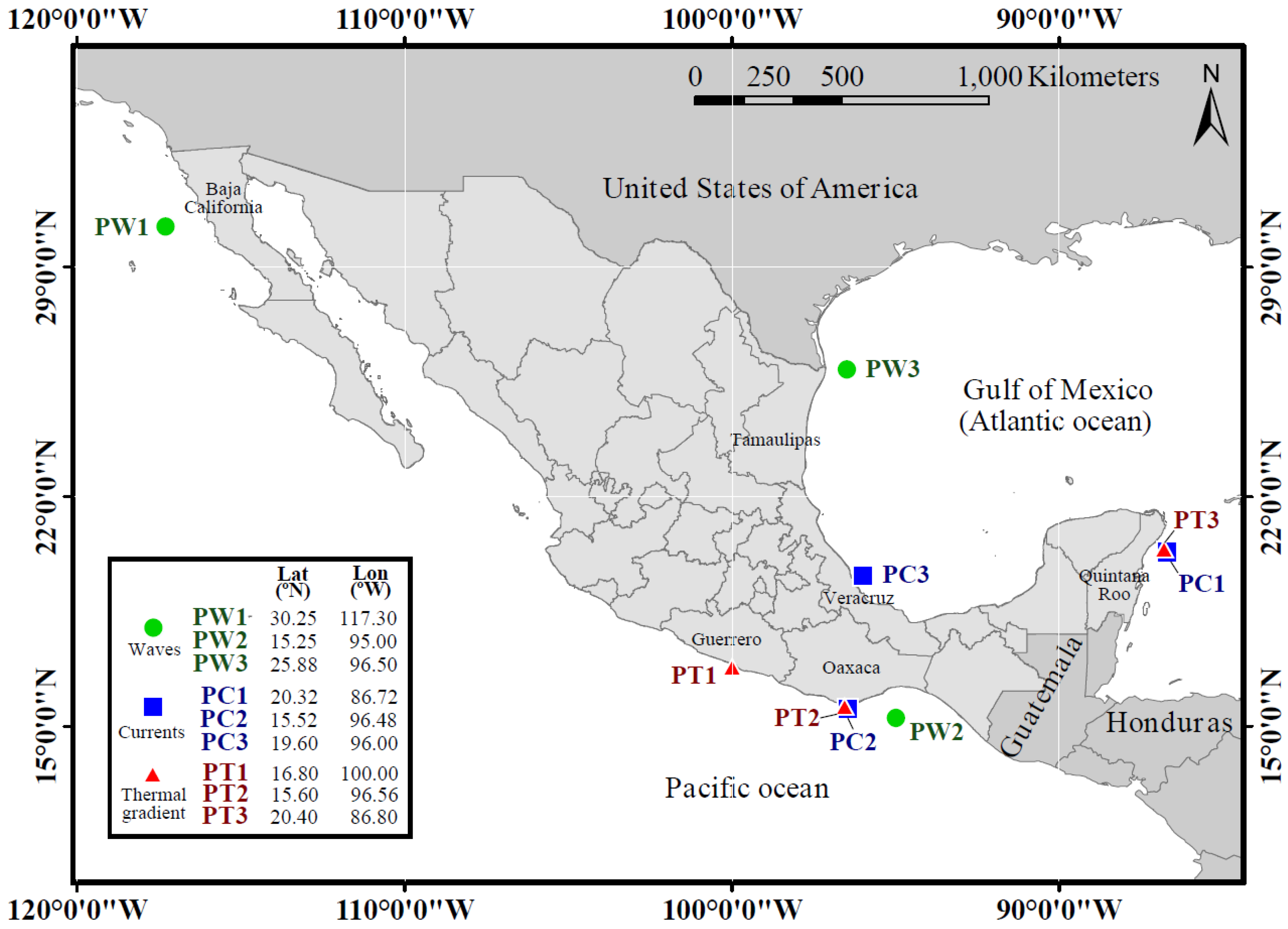
Figure 5 shows the locations of the sites considered for the present analysis. Three points were chosen to investigate the availability of power due to waves (PW1, PW2, and PW3), currents (PC1, PC2, and PC3), and thermal gradients (PT1, PT2, and PT3). Monthly-averaged power values, obtained for the ten-year period (for waves) and the five-year period (for currents and thermal gradients) were taken from the databases. Figure 6 shows the mean and standard deviation values of the theoretical power for the sites for each month. Mean values were calculated from the power defined by percentile 50 (p₅₀) of the data, whereas the standard deviation was estimated from all the data. This was done to improve the analysis of the results for sites with low power availability in particular periods of time. p₅₀ was used because the probability distributions of the available data showed skewness.

Figure 6a shows the variation in power available from wave energy for PW1, PW2, and PW3. Over the time, there was more power availability at sites PW1 and PW2. This can be expected, since the results shown previously demonstrated that the areas with the highest potential for wave energy extraction are on the Pacific. All the sites had lower potential power from May to September, while the months with highest potential power were from October to April, corresponding to the dry and rainy seasons, respectively. In all months, PW3 had standard deviation values of almost p₅₀, mainly attributed to the low power persistence, which suggests that there were some periods when not enough power was available for extraction.

Figure 6b shows the potential current power for the three sites chosen for analysis. As expected, PC1, off Quintana Roo, had the highest and most constant power availability through time, with a maximum of ~1.27 ± 0.61 kW/m² in April, and minimum ~0.45 ± 0.25 kW/m² in December. The mean values are always higher than the standard deviation, which suggests persistent availability. On the other hand, PC2 and PC3, near Oaxaca and Veracruz, respectively, had less power and more variability, as inferred from the almost equal values of p₅₀ and the standard deviations. Understanding this variability in behaviour is helpful when planning the deployment of devices in these regions. Further research should be carried out to choose the periods in which the maximum available energy can be extracted.

Figure 6c shows the potential power availability for thermal gradient energy. The three points were examined (PT1: near Guerrero, PT2: near Oaxaca, and PT3: near Quintana Roo), showing similar, persistent availability of potential energy, as can be inferred from the smaller standard deviation of the results compared with the p₅₀ values. This was expected, since it was verified earlier that there was stable power availability here. Figure 6c shows that there is an almost constant availability all the time at the three locations. Overall, power for these sites ranged from ~271 to ~361 MW for the period considered.

The results obtained for the energy sources analysed show two types of power variation for the prospective sites. In the first, the site has significant, constant power available all the time, with the p₅₀ power values always higher than the standard deviation. The second type of power variation has significant variability over time—the standard deviation values are very close to the p₅₀ values. This underlines the need for further research when planning energy extraction projects in zones where the energy resource might be available only at certain times.

6. Environmental, Economic, and Social Factors to Be Considered

As previously defined, the theoretical potential of any ocean energy source is the physical maximum usable energy in a particular region, in a specific period of time [51]. However, in practice, only part of the theoretical potential can be harnessed due to environmental, economic, and social factors that have to be addressed. In this section, some of the factors that could be relevant to projects in Mexico are briefly described.

Table 2. Main environmental, economic, and social factors to be considered in ocean energy extraction projects in Mexico, for wave, current, salinity gradient, and thermal energies.

Type	Topic	Main Concerns	WEE/CEE/SGEE/TGEE
Environmental factors	Air	Gas emissions	○/○/○/○
		Suspended particles	○/○/○/○
	Water	Changes in water temperature and salinity	○/○/◐/◐
		Water pollution by chemicals emitted by machine parts	◐/◐/◐/◐
		Changes in water hydrodynamic properties (i.e., currents and waves)	◐/◐/○/○
	Topography/Geology	Sediment transport	○/○/○/○
		Erosion	◐/◐/◐/◐
		Earthquake risks	◐/◐/●/●
	Device performance	Noise/vibration	◐/●/◐/●
		Turbulence	○/●/○/○
		Electromagnetic effects of power lines	●/●/●/●
		Attachment of marine life	◐/◐/◐/◐
		Striking some species by moving parts	◐/●/○/○
	Ecological impacts	Affectation in migration routes	●/●/○/◐
		Affectation to sanctuaries preservation	◐/◐/◐/◐
		Affectation to species in danger of extinction	○/○/○/○
	Hazards	Hurricanes/storms	◐/◐/●/●
		Earthquakes	◐/◐/◐/◐
		Tsunamis	◐/◐/●/●
Economic Factors	Recreation/Tourism	Terrestrial activities in coasts	○/○/◐/◐
		Marine activities (at sea surface)	●/◐/◐/◐
		Submarine activities	◐/●/◐/●
	Traffic/Transportation	Access to land transportation	○/○/●/●
		Access to shipping transportation	●/●/◐/◐
	Supplies necessities	Requirement of other types of energy (e.g., batteries, lubricants, fossil fuels)	◐/◐/◐/◐
		Fresh water/Refrigerants	○/○/○/●
	Available infrastructure	Proximity to a grid connection	●/●/●/●
		Maintenance/Inspection	●/●/●/●
		Requirement of a monitoring station	●/●/●/●
		Access to transportation routes	●/●/●/●
Social factors	Social acceptance	Job opportunities	●/●/●/●
		Preserve regional culture and traditions	●/●/●/●
		Adaptation of people to new activities (e.g., coastal habitants, marine workers)	◐/◐/◐/◐
	Land use	Fisheries (ships, factories)	●/●/●/●
		Recreation/Tourism	●/●/●/●
		Aquaculture activities	◐/◐/◐/◐
		Military activities	●/●/●/●
		Traffic/Transportation	●/●/◐/◐
	Human participation	Support of federal government, including its dependences	●/●/●/●
		Support of local and regional authorities	●/●/●/●
		Collaboration with academics to include research activities	●/●/●/●
		Collaboration with industry	●/●/●/●
	Security	Zones of drug trafficking	○/○/◐/◐
		Risks due to vandalism	◐/◐/●/●
		Risks due to wild life	○/○/○/○

WEE, CEE, SGEE, and TGEE refer to wave, current, salinity gradient, and thermal gradient energy extraction, respectively. ○—low; ◐—medium; ●—high.

lists some of these factors for energy extraction from waves, currents, salinity gradients, and thermal gradients. Some of them are mentioned elsewhere, in studies on the impact assessment of ocean-related projects, such as [66,67].

Each of the concerns listed in Table 2 has been evaluated qualitatively for each type of ocean energy, according to the level of required attention (low, medium, or high attention required). This preliminary assessment was performed based on the authors’ point of view, and further research must be done to address the concerns in more detail. From the factors common to all the energy sources, it is possible to summarise the following:

Environmental factors: First, it is important to consider water pollution, due to chemicals emitted by machine parts, and to evaluate the geological characteristics of the sites in case of erosion or earthquake. Then, it is worth examining the electromagnetic effects of power lines and the possibility of marine life attaching onto the devices. Finally, it is crucial to verify the effects on protected zones and to perform predictions regarding the occurrence of hazards that are common in Mexico, such as storms and hurricanes.

Economic factors: Minimisation of the interference from recreational, tourism, and transportation activities is required. The required supplies for the operational activities of the devices must be done. Proximity to the national grid and control stations is crucial for the development of projects. Specific infrastructure sites (e.g., islands, small towns, or marine facilities) must also be taken into account, including the need for appropriate maintenance services and access to transportation routes.

Social factors: First, it is important to promote the approval of the community for the activities to be carried out, preserving the culture and traditions of the region. It is also very important to consider areas which are potential zones of recreation, transportation, aquaculture, or military activities. Moreover, it is crucial to count on academic, government, and industrial participation in the projects. Finally, security factors should be considered where the sites are affected by human migration, criminal activities, and so on.

From Table 2, it can be inferred that several economic and social factors might require significant attention in the development of ocean energy projects in Mexico. It has to be considered that the results are qualitative, although they could be useful in the performance of future energy extraction evaluations.

7. Conclusions

A theoretical evaluation of ocean energy resources that could be an alternative to the use of fossil fuels in the seas around Mexico was performed. The main objective of this paper was to provide a theoretical estimation of available power from waves, ocean currents, thermal gradients, and salinity gradients, in order to set the basis for the selection of sites where further technical studies should be performed. The theoretical estimations of the power available were made through engineering approaches, using databases of simulated and measured parameters available in the literature. Moreover, some environmental and socio-economic constraints for the development of marine extraction projects in Mexico were discussed.

With respect to wave energy, the highest availability was found to be in the Pacific Ocean, where persistent wave power in the range ~2–10 kW/m can be found for more than 50% of any year. Places recommended for energy extraction are near the coasts of the states of Baja California, Baja California Sur, Jalisco, Colima, Michoacán, Guerrero, and Oaxaca.

For the case of energy from currents, the most convenient places for energy extraction were found off the Quintana Roo coast, in the Atlantic Ocean, where it is possible to find at least 32–512 W/m² of power availability more than 50% of the year. Other places with persistent power availability were found off Oaxaca, in the Pacific Ocean. At least ~32–176 W/m² of power could be extracted, 50% of the time. However, the distance to the coast could be a limitation for projects.

Energy extraction from thermal gradients seems most convenient at some places on the Pacific Ocean. It is worth remembering that this estimation was made assuming a 100 MW OTEC plant and considering an available depth of 1000 m to estimate the thermal gradient. Thermal gradient energy could be best exploited in the southwest of Mexico, in regions near the coasts of Jalisco, Colima, Michoacán, Guerrero, and Oaxaca, as well as in Quintana Roo, where power of ~100–200 MW can be found 70% of the time. It is recommended that the characteristics of pipelines and pumps for different types of power plants be included in the estimation. In addition, the efficiency of operation of specific types of plants, perhaps of lower capacity, should also be analysed.

The results for salinity gradient energy suggest that river mouths on the Gulf of Mexico, particularly in the states of Veracruz and Tabasco have the most potential for energy extraction, where sites with 564.2–4103.0 MW were identified. In Tabasco, the river Usumacinta has the highest energy potential in the country, ~4103.01 ± 683.5MW. This estimation agrees quite well with those made previously by other authors [17]. Further research should be done to evaluate the possibilities of salinity gradient energy extraction in river–lake systems and in all the river–ocean systems of Mexico. Furthermore, additional methods to improve the present estimations and to access more detailed river discharge data are recommended.

In practice, only part of the theoretical power estimated in this work can be extracted, since there are several environmental, economic, and social constraints that would have to be overcome. Even so, it has been shown that Mexico has the opportunity to take advantage of several forms of ocean energy, which can be an alternative to improve its sustainable development. It is expected that the present study will serve as a starting point for more detailed evaluations of power, which can be extended to use different estimation methods and higher-resolution input data.