Article

South Florida’s Encroachment of the Sea and Environmental Transformation over the 21st Century

1
Physical Resources, South Florida Natural Resources Center, National Park Service, Homestead, FL 33030, USA
2
Biological Resources, South Florida Natural Resources Center, National Park Service, Homestead, FL 33030, USA
*
Author to whom correspondence should be addressed.
J. Mar. Sci. Eng. 2017, 5(3), 31; https://doi.org/10.3390/jmse5030031
Submission received: 12 April 2017 / Revised: 10 July 2017 / Accepted: 18 July 2017 / Published: 28 July 2017
(This article belongs to the Special Issue Coastal Sea Levels, Impacts and Adaptation)

Abstract

:
South Florida encompasses a dynamic confluence of urban and natural ecosystems strongly connected to ocean and freshwater hydrologic forcings. Low land elevation, flat topography and highly transmissive aquifers place both communities at the nexus of environmental and ecological transformation driven by rising sea level. Based on a local sea level rise projection, we examine regional inundation impacts and employ hydrographic records in Florida Bay and the southern Everglades to assess water level exceedance dynamics and landscape-relevant tipping points. Intrinsic mode functions of water levels across the coastal interface are used to gauge the relative influence and time-varying transformation potential of estuarine and freshwater marshes into a marine-dominated environment with the introduction of a Marsh-to-Ocean transformation index (MOI).

1. Introduction

Sea level rise is not evenly distributed around the globe, and the response of a regional coastline is highly dependent on local natural and human settings [1]. This is particularly evident at the southern end of the Florida peninsula where low elevations and exceedingly flat topography provide an ideal setting for encroachment of the sea. Coastal South Florida is fringed by national parks including Biscayne and Everglades National Parks, Big Cypress National Preserve and the islandic Dry Tortugas National Park. This rich natural setting and subtropical climate appeal to human interests with over six million inhabitants residing along narrow coastal strips along the Atlantic and Gulf coasts. The sustenance of these natural and human ecosystems is predicated on adequate freshwater supply, and while South Florida receives an average of 140 cm of rainfall annually, losses to evaporation are nearly as great as the rainfall itself, and water storage is limited to shallow, permeable reservoirs and thin surficial aquifers that are experiencing diminishing capacity as rising sea level drives saltwater infiltration.
Attempts to control the hydrologic resources have resulted in the construction of one of the most complex and expansive water control projects on the planet with both beneficial and detrimental impacts on human and natural populations [2,3]. Regional governments recognize the need to assess and plan for sea level rise implementing a Regional Climate Action Plan [4] with a task force specifically addressing sea level rise [5]. However, these efforts focus on urban and suburban areas with concern for property values, transportation, housing, water supply and sewer infrastructure based on global sea level rise projections that do not reflect local processes and that are not associated with specific probabilities of occurrence.
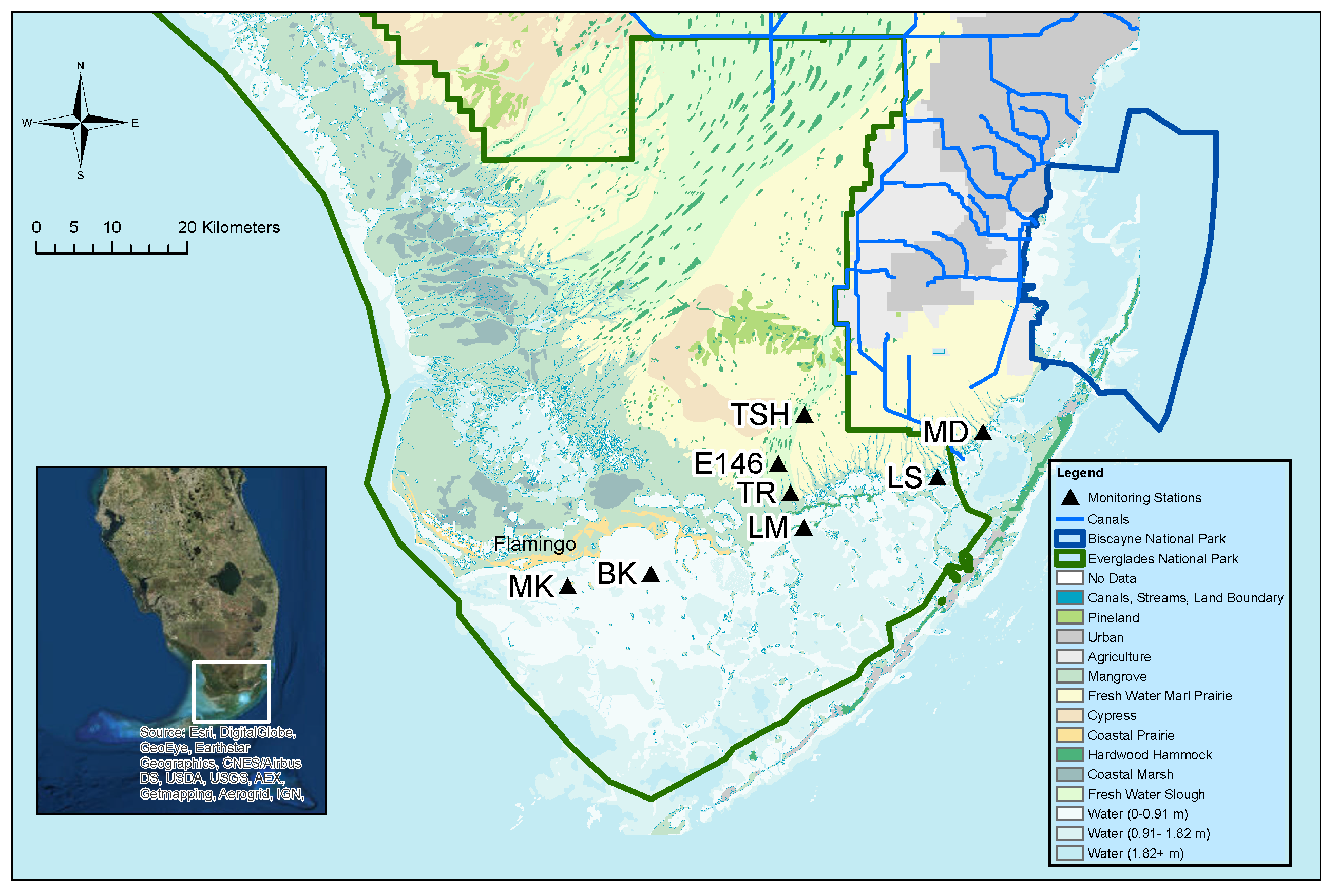
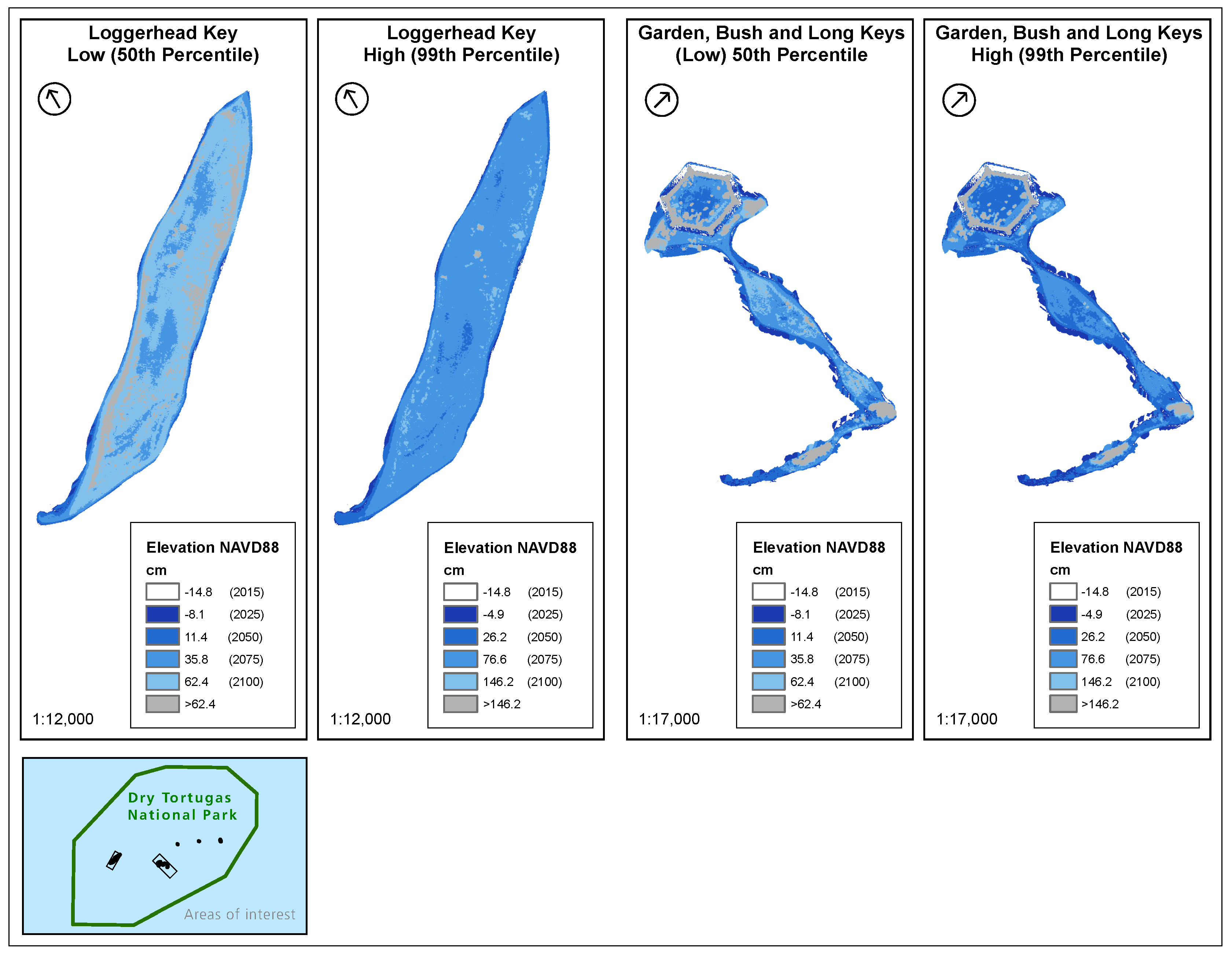
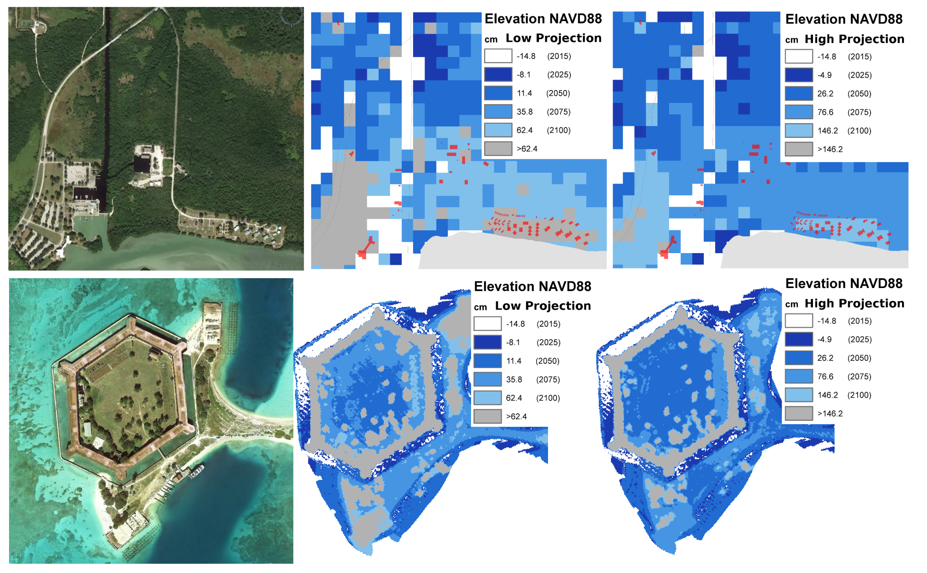
Here, we focus on the low-elevation natural areas at the southern end of the peninsula as shown in 
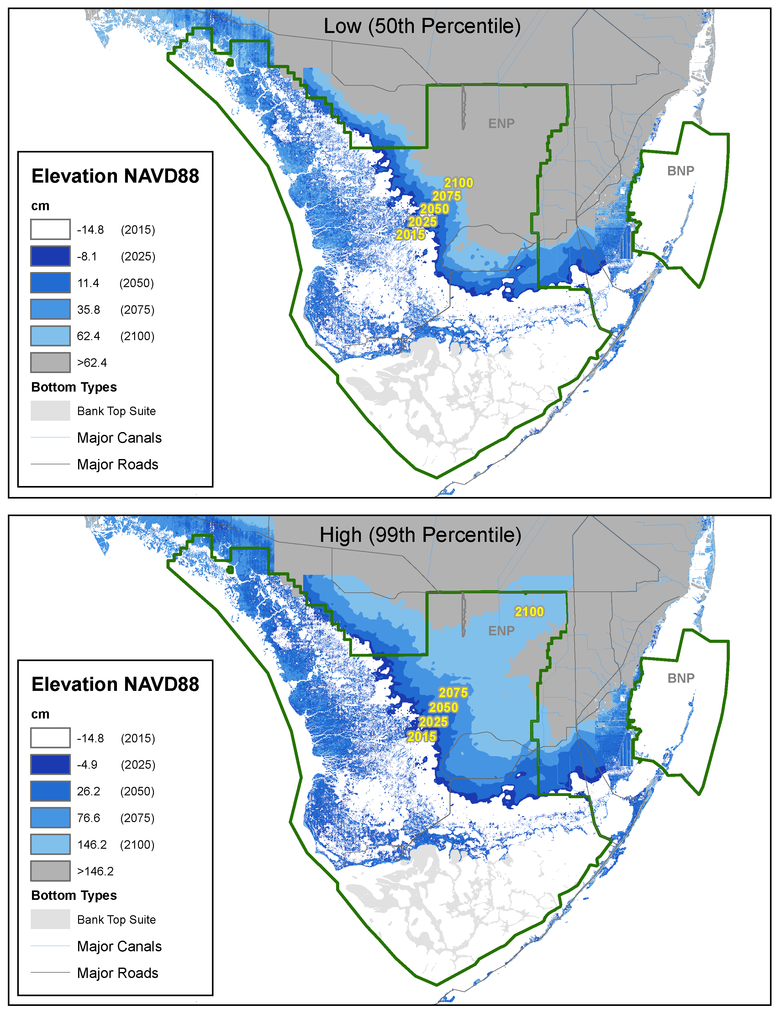
Figure 1, as these areas will experience inundation impacts prior to the urban areas, thereby serving as sensitive indicators of sea level rise. We evaluate sea level rise inundation impacts under two scenarios, a low projection and a high projection, based on a synthesis of coupled atmosphere-ocean general circulation models and tide gauge information reflecting local processes. The high projection represents an upper percentile (99%) of expected sea level rise given current models and observations, while the low projection corresponds to a median (50%) sea level rise scenario. Since models, observations and current scientific understanding are incomplete, these projections are necessarily incomplete and do not account for a rapid collapse of the Antarctic ice-sheets, a development that is currently unfolding with potential to render these projections as lower bounds [6,7].
We also examine coastal water level exceedance data, quantifying an exponential increase in low-elevation exceedances over the last decade. Application of the sea level rise projections allows us to project these exceedance curves into the future, where one can identify tipping points and time horizons for the transformation of coastal regions into marine ecosystems. Finally, we introduce a metric to characterize the transformation of a coastal wetland from a freshwater marsh into a saltwater marsh based on intrinsic mode functions of water level time series extending landward from the sea.

2. Materials and Methods

2.1. Sea Level Rise Projection

The Intergovernmental Panel on Climate Change’s (IPCC) most recent evaluation is the Fifth Assessment Report (AR5) [8] including projections of global sea level rise based on different Representative Concentration Pathway (RCP) scenarios reflecting possible future concentrations of greenhouse gases1. RCP 8.5, also known as the business-as-usual scenario, is the highest emission and warming scenario under which greenhouse gas concentrations continue to rise throughout the 21st Century, while RCP 6.0 and RCP 4.5 expect substantial emission declines to begin near 2080 and 2040, respectively.
The IPCC sea level rise scenarios are comprehensive, but do not include contributions from a rapid collapse of Antarctic ice sheets. However, recent evidence suggests that such a collapse may be underway [6,7]. In addition, the IPCC projections do not account for local processes such as land uplift/subsidence and ocean circulation and do not provide precise estimates of the probabilities associated with specific sea level rise scenarios.
A contemporary study that does estimate local effects and comprehensive probabilities for the RCP scenarios is provided by Kopp et al. [9] based on a synthesis of tide gauge data, global climate models and expert elicitation, including contributions from the Greenland ice sheet, West Antarctic ice sheet, East Antarctic ice sheet, glaciers, thermal expansion, regional ocean dynamics, land water storage and long-term, local, non-climatic factors, such as glacial isostatic adjustment, sediment compaction and tectonics. Even though this model includes contributions from the Antarctic ice sheets, these contributions are from dynamic equilibrium models and do not yet account for an incipient rapid collapse as noted above. Nonetheless, we find the Kopp et al. [9] projections to be among the most mature and useful sea level rise paradigms and base our South Florida projections on their results at Vaca Key, Florida.

South Florida Sea Level Rise Projection

Examination of local sea level rise projections around South Florida finds small differences between Naples, Virginia Key, Vaca Key and Key West. We chose the Vaca Key station sea level data as representative of South Florida since they best reflect local oceanographic processes that influence coastal sea levels [10].
Next, we select the RCP scenario that best fits our understanding for future greenhouse gas emissions. Although significant effort is aimed at global emission reduction, atmospheric CO 2 and emissions continue to escalate [11], and there is presently no clear socio-economic driver to depart from a carbon-based energy infrastructure. Further, recent assessments of global energy production and population conclude that the the achievement of emission scenarios corresponding to a desired 2 °C limit in global mean temperature increase require the global fraction of Renewable Energy Sources (RES) to reach 50% by 2028 [12].
We note that the International Energy Agency (IEA) reports that global RES could reach 28% by 2021 [13]. This is consistent with a 2015 estimate of 24% RES by the United Nations [14] and, if accurate, would leave seven years to achieve a near doubling to 50% to meet the Jones and Warner [12] constraint. Currently, RES is dominated by hydropower, a resource that is not easily scalable or quick to bring online. In the absence of a technological breakthrough, we conclude it is unlikely that global RES will reach 50% by 2028. This leads us to expect that the RCP 4.5 emission scenario is unobtainable and that there is significant uncertainty as to whether the RCP 6.0 scenario can be realized. We therefore restrict our projection to the RCP 8.5 scenario.
Finally, we select conservative projection probabilities appropriate for informing authorities of anticipated sea level rise for adaptation and planning purposes. In light of the significant uncertainties inherent in the generation of the projections and future climate dynamics, it is prudent to consider the upper percentile range of projections leading us to select the RCP 8.5 median (50th percentile) as the lower boundary and the 99th percentile as the upper boundary. Although the high projection is deemed to have a 1% chance of occurrence under current climate conditions and models, in the event of Antarctic ice sheet collapse, this high projection is consistent with estimates of the Antarctic ice melt contribution [15].
The resultant sea level rise projection for South Florida referenced to the North American Vertical Datum of 1988 (NAVD88, Appendix A) is shown in Figure 2 and tabulated in Appendix B. Projection starting points have been offset to coincide with observed mean sea level in Florida Bay over the period 2008–2015 (Appendix C). The projection does not incorporate local processes such as tides, storm surges, waves or their non-linear interactions with inundation impacts, issues that are discussed in Appendix D.

2.2. Inundation Coverage

Geospatial inundation coverages for mean sea level are created in ArcMap by application of the sea level rise projections for the years 2025, 2050, 2075 and 2100 across southern Florida. Topographical elevations are based on a synthesis of the best available high-resolution digital elevation data [16] with variable spatial resolution, but a nominal horizontal grid cell size of 50 m. The resulting inundation coverages represent a static land-masking of mean sea level at the four time horizons and do not represent influences from tides, seasonal oceanographic cycles, teleconnections, weather, such as storms, or inverse barometric adjustments, as discussed in Appendix D, or for changing morphological structure in submerged and inundated sediments or hydraulic connectivity [17]. A review of these issues and how the dynamic effects of sea level rise interact with low-gradient coastal landscapes can be found in Passeri et al. [18].

2.3. Water Level and Salinity

Water levels are obtained from eight hydrographic stations operated by Everglades National Park over the period 1 June 1994–31 December 2016 with station locations and names shown in Table 1. Water levels are collected at 6-, 15- or 60-min intervals by WaterLog shaft-encoded float gauges recorded by a Sutron SatLink2 data recorder. Water levels are then aggregated into daily mean values as shown in Figure 3.
Salinity is estimated from specific conductivity measured at 30- or 60-min intervals by a YSI 600R Water Quality Sonde and application of the International Equation of State of Seawater 1980 and Practical Salinity Scale 1978 as recommended by the United Nations Educational, Scientific and Cultural Organization (UNESCO) Joint Panel on Oceanographic Standards and Tables [19]. Daily mean salinities are shown in Figure 4, and summary statistics of the water level and salinity time series are presented in Table 2.

2.4. Empirical Mode Decomposition

Water level and salinity data are decomposed into Intrinsic Mode Functions (IMFs) and nonlinear trends through Empirical Mode Decomposition (EMD) using the Hilbert–Huang transform [20,21] as implemented in the R package hht. Application of the EMD requires uniformly-sampled data without gaps. We reconstruct missing data in our time series by using random samples drawn from distributions of all available data for a specific year day. For example, if 1 January 2000 is missing, a Gaussian kernel is fit to all available data for 1 January. A random sample is then drawn from this distribution and used as the reconstructed value. This preserves the overall distribution of the data for a year day capturing seasonal trends, while realistically allowing for variance away from the mean on the daily timescale.

2.5. Water Level Exceedance

Water level exceedances are computed from daily mean water levels by summing the number of exceedance events above an elevation threshold for each year. The probability of exceedance at a specific threshold as a function of time follows a logistic function exhibiting exponential growth followed by a linear increase, terminating in nonlinear saturation as water levels continuously exceed the threshold [22]. The logistic function suggests a growth model for water level exceedances as they enter the initial growth phase:
E ( t ) = E 0 + α ( t T L ) + ( 1 + r ) t T G τ
where E 0 is the number of exceedances at year t = 0 ; α the linear rate of exceedance; r the growth rate; T L and T G the zero-crossing time of linear and exponential growth, respectively; and τ the growth time constant. This model is fit to yearly exceedance data with maximum likelihood estimation over a wide parameter space of initial conditions (Table 3), and the best-fit model from the parameter search is selected based on the minimum Akaike information criteria [23].
To forecast the evolution of water level exceedance, we select an elevation threshold with landscape-specific relevance. For example, at the Little Madeira Bay (LM) station, inspection of coastal ridge elevations from the United States Geological Survey (USGS) mapping [24] finds a mean elevation of 70 cm NGVD29. Daily mean water levels are then extracted from the station data for the most recent three-year period, and yearly values of sea level rise from the low and high sea level rise projections are added to the dataset. Each set of yearly data is then processed to sum the total number of yearly threshold exceedances per year.

2.6. Marsh to Ocean Transformation Index

As sea levels rise, we expect a gradual transformation of freshwater coastal marshes into saltwater marshes and eventually into submarine basins. Florida Bay is largely open to the Gulf of Mexico to the west and relatively isolated from the Atlantic Ocean to the east by the island chain of the Florida Keys; as such, marine conditions can be found in western Florida Bay as shown by the tidally-dominated water levels at Buoy Key (BK) (Figure 3) and marine-like salinities at Murray Key (MK) and Buoy Key (Figure 4). As one moves eastward, the tidal signal diminishes (LM in Figure 3) with a transition to a terrestrial hydrologic cycle dominated by seasonal rainfall moving up Taylor Slough (Taylor River (TR), E146 and Taylor Slough Hilton (TSH)).
To assess this change, we decompose the water level signals shown in Figure 3 using IMFs retaining only modes with intra-annual and longer oscillatory cycles, as shown in Figure 5. These low pass versions of water levels allow one to recognize lower amplitude ocean-dominated locations such as Buoy Key (BK) and the higher amplitude, more variable marsh-dominated water levels exemplified at TSH.
We next identify IMFs representing ocean-dominated and freshwater marsh-dominated locales at BK and TSH, respectively, as shown in Figure 6, and use these IMFs as empirical basis functions to reconstruct the low pass water level signals at the intermediate stations LM, TR and E146. The reconstruction is based on linear combinations of weighted ocean and marsh basis functions with the goal of comparing the relative magnitudes of the ocean and marsh basis function fit coefficients as a metric describing the relative hydrologic influence of the marsh or ocean at a particular station.
The model is thus:
W ( t ) = i = L i = H ω i I M F Ω i + μ i I M F M i
where I M F Ω represent ocean-dominated empirical basis functions, I M F M marsh-dominated basis functions, L the IMF mode number of the lowest frequency mode or residual, H the mode number of the highest frequency mode and ω i and μ i fit coefficients determined by a nonlinear quasi-Newton minimization of the variance of the difference between the weighted sum of the empirical basis functions, W ( t ) , and the target time series (low pass signal of station LM, TR or E146 shown in Figure 5) [25].
The resultant coefficient vectors ω and μ are summed to produce an overall metric Ω = ω i , M = μ i representing the ocean or marsh influence. For example, with N = 3 empirical basis functions and using the Buoy Key (BK) time series as the target, all ω i equal 1 with the result Ω = 3 , M = 0 , while if TSH is the target then Ω = 0 , M = 3 . To construct a relative metric denoted as the Marsh-to-Ocean Index (MOI), we normalize the difference of the two influence metrics by the number of basis functions N:
MOI = M Ω N
so that a water level signal identical with that of Buoy Key (BK) would express MOI = −1, while a station with a signal equivalent to the upper reach of Taylor Slough (TSH) would produce MOI = 1.
The MOI discriminates between ‘oceanic’ and ‘marsh’ water level variations based on the assumption that variations in the designated ocean signal represent ocean forcing, and likewise for the marsh signal. Implicitly, a storm surge elevating coastal water levels at the ocean station is characterized as an ocean influence, while a runoff event from storm rainfall at the marsh station is attributed as a marsh water level forcing. Here, we are interested in assessing long-term transformations in hydrologic responses, basing MOI low-pass signals on intra-annual and longer cycles. The MOI methodology is general such that inclusion of higher-frequency IMFs that resolve temporally-compact events should be properly accounted for as originating from either the oceanic or marsh reference signals. The time period over which the ocean and marsh basis functions are fit to the intermediate station can also be varied to emphasize shorter-term events or longer-term processes.

3. Results

3.1. Inundation Maps for Mean Sea Level

Figure 7 and Figure 8 present mean sea level inundation maps for the southern Florida peninsula and Dry Tortugas. Blue shadings represent the extent of projected mean sea level inundation at the four time horizons of 2025, 2050, 2075 and 2100. Grey areas indicate elevations higher than the expected mean sea level at 2100. Note that the low and high projections do not share a common legend such that the shade of blue corresponding to a specific land elevation is not shared between the low and high projections; however, the time horizon at which mean sea level reaches an elevation does correspond to the same shade of blue in both projections. Digital versions of the inundation maps are available in the Supplementary Materials.

3.1.1. General Influence of Sea Level Rise

Over the next ten years, represented by the 2025 estimates, dramatic change in sea level is not anticipated with an expected sea level rise of 7 cm for the low scenario and 10 cm for the high projection. These changes will result in more frequent tidal inundation along coastal regions although the buttonwood ridge located along the southern peninsula and north shore of Florida Bay should remain above mean sea level. This modest increase is not likely to impact the terrestrial portions of South Florida or the Dry Tortugas.
By 2050, local sea levels are expected to increase between 26 and 41 cm. Overall, inundation at mean sea level will produce similar impacts for both scenarios with a wider fringe of saltwater inundation around the periphery of the peninsula under the high scenario. Expansion of the white zone, a low productivity area influenced by the periodic flooding of saltwater [26], is expected to continue. Under both projections, mean sea level is expected to reach the elevation of the land surrounding the Florida Power and Light Turkey Point nuclear power plant cooling canal system (vertical lines along the southwest corner of Biscayne National Park (BNP) in Figure 7).
By 2075, sea levels are anticipated to increase by 51 and 91 cm for the low and high projections, respectively. At these elevations, significant portions of the buttonwood ridge separating Florida Bay from the peninsula will be exceeded by mean sea level, and marine conditions can be expected to expand into current-day areas of the Everglades that maintain fresh and brackish-water marshes. This could signal an important tipping-point in the ecological response of freshwater marshes since freshwater basins delineated by the ridge will no longer be viable. Low-lying suburban areas along the southeastern peninsula will also be at mean sea level elevation resulting in perennial tidal flooding with significantly reduced ability to discharge rain floodwaters by gravity from the urban areas into the sea. Below ground, saltwater intrusion can be expected to reduce aquifer productivity along coastal well fields [27].
In 2100, the projected sea level rise is 77 cm for the low projection and 161 cm for the high scenario. Strikingly, in the high scenario, mean sea level can be expected to extend from the southwest peninsula to the northeast corner of Everglades National Park along the topographical depression of Shark River Slough. It is likely that widespread ecological changes will be evident around South Florida as Florida Bay expands. Many of the low-lying islands of Biscayne and Dry Tortugas national parks can be expected to become tidally submerged or dynamically redefined. Islands with coral substrate are likely to submerge, while sand- or sediment-based islands will become increasingly mobile as tidal influences trigger localized erosive and depositional dynamics.

3.1.2. Infrastructure Inundation

Figure 9 presents a comparison of projected mean sea level with land elevation surrounding infrastructure at Flamingo in Everglades National Park and Fort Jefferson in Dry Tortugas National Park where red indicates a building or infrastructure footprint. Conditions at Flamingo are mixed, with the low projection forecasting the housing and visitors center to remain above mean sea level to 2100, but with mean sea levels reaching the boat basin, maintenance yard and water plant by 2100. Under the high projection, the housing area is at mean sea level by 2100; the visitor center will be partially inundated by 2050; and the maintenance yard and water plant by 2075.
At Fort Jefferson, the projections indicate that the north coal dock and campground remain above mean sea level to 2100, while areas around the ferry dock and the isthmus to Bush and Long Keys are expected to be at mean sea level by 2075 under the low sea level rise projection. Under the high projection, much of the north coal dock and campground will be at mean sea level by 2075, as will much of the land between the ferry dock and moat, although a portion of this will be at sea level by 2050. The isthmus to Bush Key is expected to be at mean sea level by 2050.
It is important to note that mean sea level in Florida Bay fluctuates by approximately 30–40 cm (12–16 in) in a yearly oceanographic cycle, as well as up to 70 cm (2.3 ft) in daily and monthly tidal cycles so that effects of tidal inundation will be observed during high tides several years before the projected dates when mean sea level reaches a specific land elevation.

3.2. Exceedances

As sea levels rise against a fixed elevation threshold near the mean high water tidal elevation, exceedance rate changes will follow Equation (1) experiencing nonlinear growth regardless of whether water levels are increasing at a steady or accelerated rate [22]. This is exemplified in Figure 10 at four coastal stations across the southern peninsula suggesting a transition from linear exceedance growth to exponential growth. Model parameters fit to the middle elevation threshold are shown in Table 4.
Exceedance model fits suggest a progression of exponential growth initiation times ( T G ) from the eastern end of Florida Bay where freshwater marsh interaction with the coastal region is high, to the western side of the Bay where marine conditions prevail with substantial water mass exchange with the Gulf of Mexico. Generally, the transition of exceedances near the mean high water tidal threshold suggest that the late 20th to early 21st century represents a change of coastal dynamics where water level exceedances enter a growth phase. Interestingly, the model fits indicate that the doubling times ( τ ) increase from one decade in the marine areas to two and half decades in the eastern coastal region of Florida Bay, suggesting that environmental impacts from increased exceedances may be more acute over the next few decades along the southwestern coastal region.

Exceedance Projections

Application of the sea level rise projections to exceedance data has potential to provide a meaningful environmental-change metric. For example, projection of exceedances at Little Madeira Bay based on a mean local coastal ridge elevation threshold of 70 cm NGVD29 is shown in Figure 11. Several illuminating inferences can be made from this projection; for example, it suggests that regardless of whether sea levels rise along the low or high trajectory, that between the years 2035 and 2045, mean sea level exceedances will enter a phase of exponential growth. Under the high projection, it indicates that circa 2050, mean sea level will be continuously above portions of the coastal ridge wherein one would expect marine conditions to have displaced freshwater influences. If the low projection is realized, then this transition is expected near 2070.
Such exceedance projections may therefore find utility in the identification of tipping points where the transition to an exponential increase in saltwater inundation can be expected, as well as demarcation of a time horizon upon which a fundamental transformation of the coastal environment to submarine conditions will prevail.

3.3. Trends

Empirical mode decomposition of the water level and salinity data shown in Figure 3 and Figure 4 provides a residual signal representing the time-varying trend after all oscillating modes are removed as shown in Figure 12. Regarding salinity, Murray Key and Buoy Key in western Florida Bay exchange waters with the Gulf of Mexico, as well as fresh water runoff from the coastal Everglades, but are predominantly marine ecosystems. Seawater has a nominal salinity of 35 ppt, and we find that mean Murray Key salinity has risen by 2.8 ppt from 32.7 in 1994 to 35.5 ppt in 2016, with values at Buoy Key rising by 6.2 ppt from 30.6–36.8 ppt over the same period indicating that both stations are currently experiencing higher mean salinity and lower freshwater mixing than was common 20 years ago. Little Madeira Bay in the eastern coastal region is more influenced by freshwater runoff from the Everglades and agricultural lands with its mean salinity increasing by 3.2 ppt from 22.4 ppt in 1994 to 25.7 ppt in 2016.
Mean water levels are found to have increased in Florida Bay and the southern reaches of Taylor Slough as shown in Figure 12. In Florida Bay, water levels at Buoy Key and Little Madeira Bay have risen from 27.7 cm NGVD29 in 1994 to 32.7 cm in 2016, an increase of 5.0 cm, with similar increases over the period observed at the Taylor Slough stations TR and E1462.

3.4. Marsh to Ocean Transformation

As described above, the MOI is designed to represent the relative similarity of a time series spatially intermediate with respect to two reference time series representing oceanic and marsh hydrology. Specifically, the relative similitude of water levels over the last three years at Little Madeira Bay (LM) and within Taylor Slough at stations TR and E146, with respect to the oceanic reference station of Buoy Key (BK) and marsh reference at station Taylor Slough Hilton (TSH), are shown in Table 5. MOI values of −0.21 at Little Madeira Bay (LM), 0.02 at Taylor River (TR) and 0.34 in Taylor Slough (E146) suggest that recent water levels at Little Madeira Bay follow the dynamics observed at Buoy Key more closely than those of Taylor Slough (TSH), while levels at E146 are more similar to TSH dynamics.
To assess changes in behavior over time, we apply the MOI to the three intermediate stations LM, TR and E146 over a one-year moving window advanced in 10-day increments, as shown in Figure 13. Also shown in Figure 13 is the monthly accumulation of streamflow measured at the confluence of the Taylor River and Little Madeira Bay. This flow represents a fraction of total flow as freshwater into Little Madeira Bay, but is representative of the annual hydrologic cycle driving marsh hydrology. For example, the large flow in 2005 associated with hurricanes Katrina and Wilma resulted in an increase in MOI at Little Madeira Bay from negative to positive values. Overall, it is difficult to discern patterns in the MOI dynamics, although it does appear that since 2012, MOI has remained largely positive at the Taylor River (TR) and Taylor Slough (E146) stations.
Since the effects of environmental and hydrologic perturbations on the biomes, landscapes and ecosystems are cumulative, it makes sense to view the cumulative behavior of the time-varying MOI. In Figure 14, we plot the time integral of the MOI shown in Figure 13, that is: 0 T MOI ( t ) d t , where T is a specific day past the data origin of 1 June 1994. This integrated view of the dynamics suggests varying responses at the three stations. At Little Madeira Bay along the coastal interface between Florida Bay and the confluence of Taylor Slough, the MOI exhibits an increasing oceanic influence from 1994–2004 followed by a stable, but still negative MOI over the 2004–2013 period punctuated by the 2005 freshwater event. At the Taylor River station a stable, near-zero MOI from 1994–2000 transitioned to a steady decline from 2000–2012, followed by an increasing trend. At station E146 in Taylor Slough, the cumulative MOI has been steadily increasing since 1994.
Our interpretation of these results is that northern Florida Bay has been transitioning away from a freshwater marsh estuarine environment towards a marine environment over the last two decades. While this transition appears to be essentially continuous in Little Madeira Bay since 1994, at the lower reach of Taylor Slough (TR), hydrologic cycles appear to be transforming from marsh-dominated dynamics to ocean-dominated since 2000. These shifts in hydrologic cycles are consistent with increasing mean sea level (Figure 12) and the onset of accelerated water level exceedances as sea level rises (Figure 10). In the middle-reaches of Taylor Slough represented by station E146, there were periods of negative MOI during 2003 and 2006 (Figure 13) reflected in a stasis of the integrated MOI over this period (Figure 14), but the overall assessment is that there is no evidence of emerging ocean-dominated hydrologic cycles.

4. Discussion

South Florida is ranked ninth globally among urban areas with human populations exposed to sea level rise impacts and first in terms of exposed assets [28]. South Florida is equally rich in natural assets with national parks circumscribing the southern peninsula protecting vital freshwater ecosystems that sustain both natural and human biomes. The exceedingly flat topography and low elevations provide ideal conditions for the expansion of marine bays and estuaries into existent freshwater marshes, civil infrastructure and human habitats, issues recognized by regional governments planning for future sea levels. Such planning efforts rely on global projections without a probabilistic estimate of sea level likelihood, and focus on urban areas. Here, we examine projected impacts based on a local sea level rise projection with explicit probabilities corresponding to the median and 99th percentiles focusing on the estuarine coastal fringe along the southern end of the peninsula. This fringe is generally lower in elevation than the urbanized east coast, and its natural condition provides an optimal setting to monitor sea level rise and landscape transformation.
Inundation projections indicate dramatic changes in landscape along the southern peninsula over the 21st century with the submergence of low-lying urban and suburban areas, as well as land surrounding cooling canals at the Turkey Point nuclear power plant. In the Everglades, it appears that substantial portions of existent freshwater marshes will be converted to estuarine and shallow marine zones with the potential for mean sea level to span the interior of the peninsula along Shark River Slough.
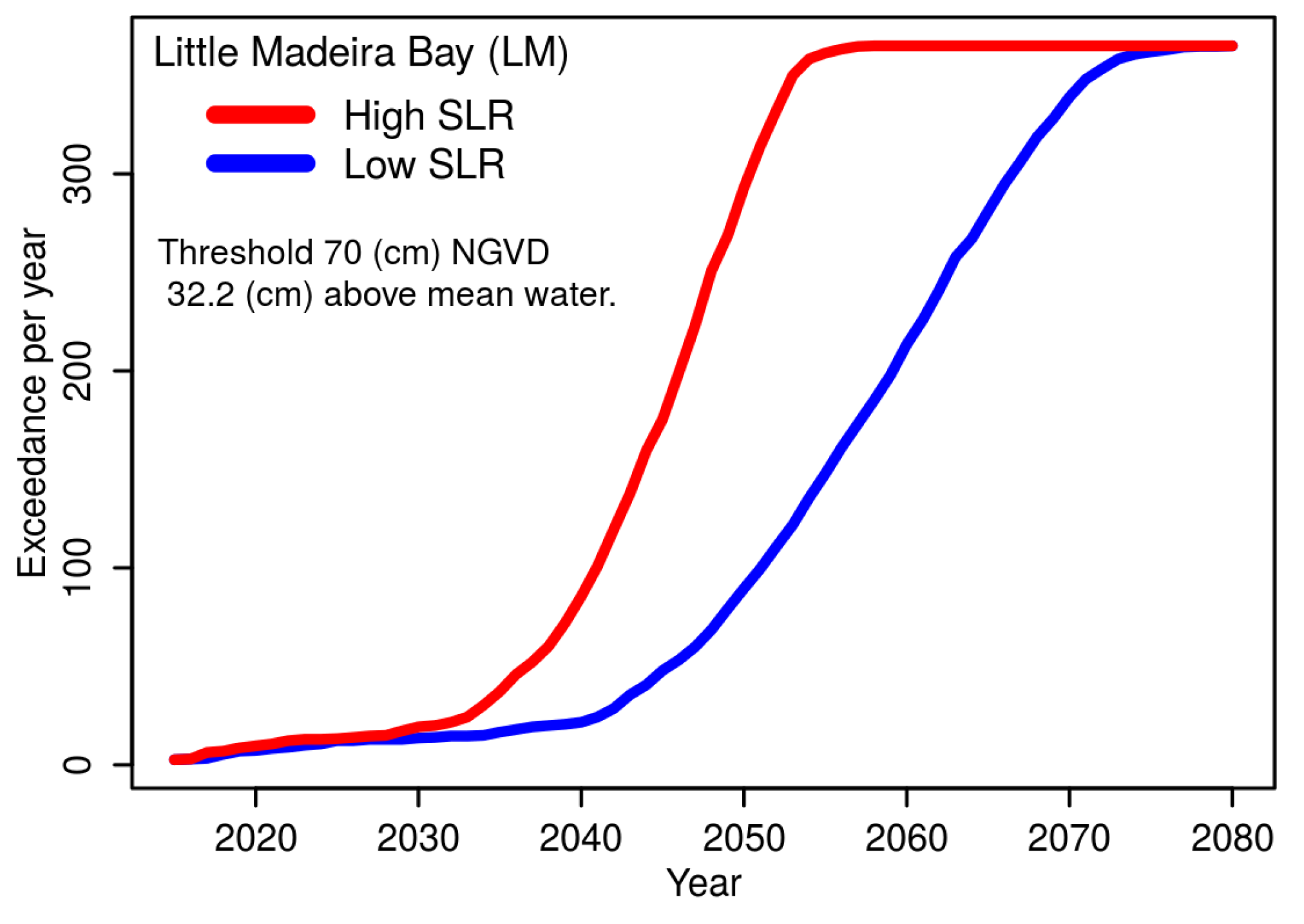
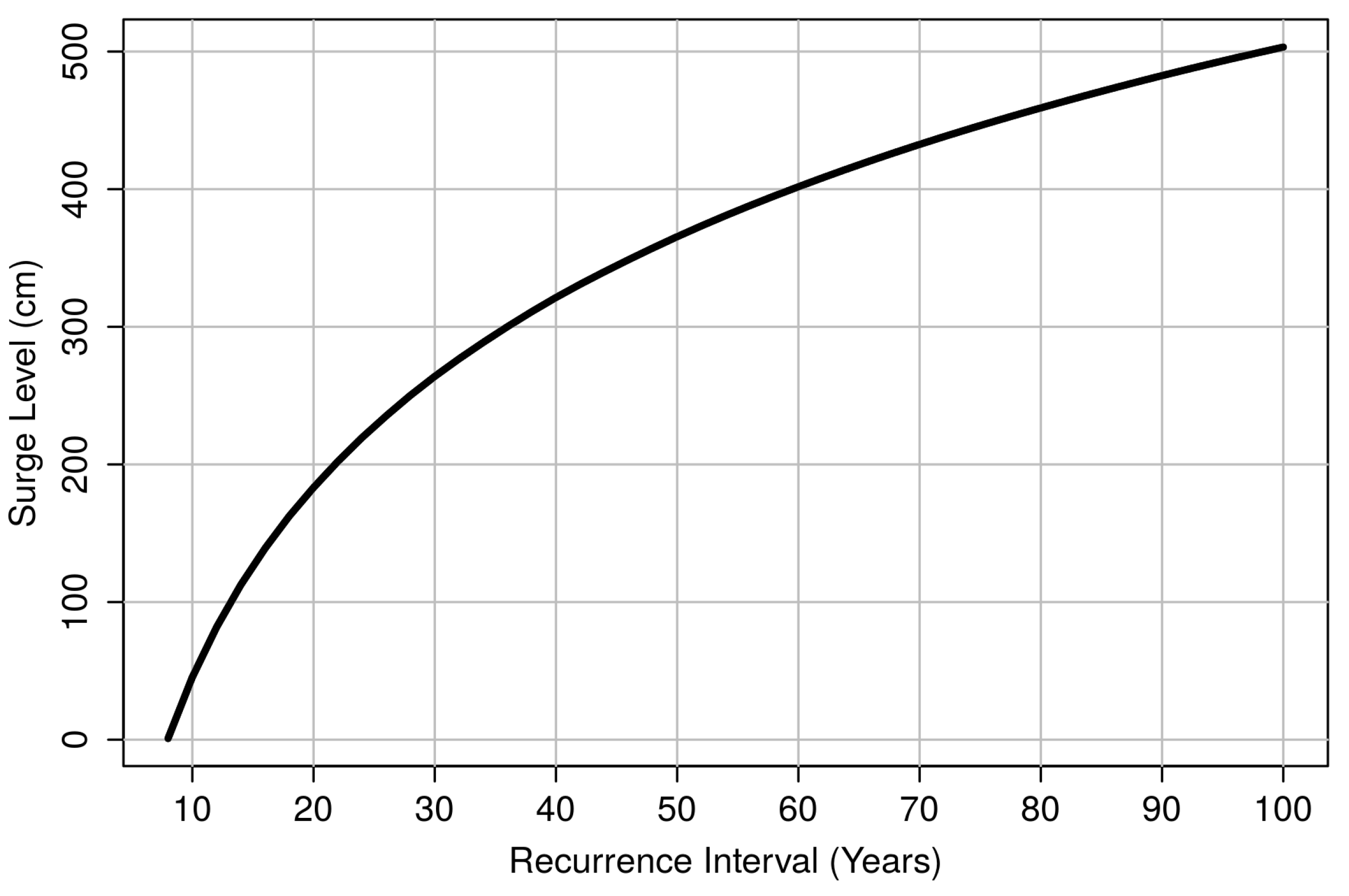
A fundamental landscape feature of the southern peninsula is a low, narrow ridge separating the marine and estuarine waters of Florida Bay from freshwater marshes of the southern Everglades. When sea levels rise above this ridge, a pronounced environmental transformation into a marine-dominated landscape is expected. We can anticipate this change by applying sea level rise projections to recent exceedance statistics at the ridge elevation to identify a tipping point horizon where water level exceedances above this elevation will grow, as well as when the elevation is forecast to become submarine, signaling a complete transformation to marine or estuarine conditions. Doing so, we find that circa 2040, the coastal region of Little Madeira Bay will enters the transition of accelerating water level exceedances above the coastal ridge, and between 2050 and 2070, the area is expected to be transformed into a marine-dominated landscape.
Transformations along the southern peninsula are inexorably coupled to ecological changes and feedbacks with the coastal landscape consisting of a dynamic surficial layer of wetland soil overlying a karstic surficial aquifer. Freshwater soils of mostly organic-rich peat support the ridge-and-slough landscape and tree islands, while coastal wetlands such as salt marshes and mangroves contain substantial organic matter along with varying amounts of inorganic sediment washed in by tides, waves or storm surge. The conversion of coastal marshes to open water from saltwater intrusion and sea-level rise is often accompanied by peat collapse and deterioration, releasing large amounts of sequestered carbon. It is estimated that mangrove forests in the Everglades store 145 tonnes per hectare [29].
These coastal wetlands possess a limited capacity to stabilize and maintain existing coastal barriers through accretion of organic matter and storm-derived sediment with an average accretion rate of 1–3 mm/year with more rapid accretion rates possible for short periods of time [30]. Global rates of sea level rise are currently estimated at 3.4 mm/year [31], and our data find local rates of 4 mm/year over the last decade. In view of the established and expected acceleration of sea level rise, the landscape may have reached a tipping point unable to sustain spatially-static coastal mangrove forests. Indeed, vegetation loss along the coast is expressed in a “white zone” of low productivity that has been shifting inland over the past 70 years [3,32], and models of expected mangrove proliferation suggest that a 66-cm sea level rise corresponding to year 2070 under the high sea rise projection and 2100 under the low scenario will transform 2000 square kilometers of freshwater marsh into mangrove forests [33].
While inundation projections point to expected changes, examination of water levels allow us to detect and quantify an acceleration of water level exceedances over the last decade. Such an acceleration is a natural product of rising sea levels against a fixed elevation whether the change in sea level itself is linear or accelerating, and we find that exponential doubling times for these exceedances are on the order of one to two decades. Ecological transformation from freshwater to saltwater biomes is driven by the spatial and temporal extent of these saltwater inundations, and in 
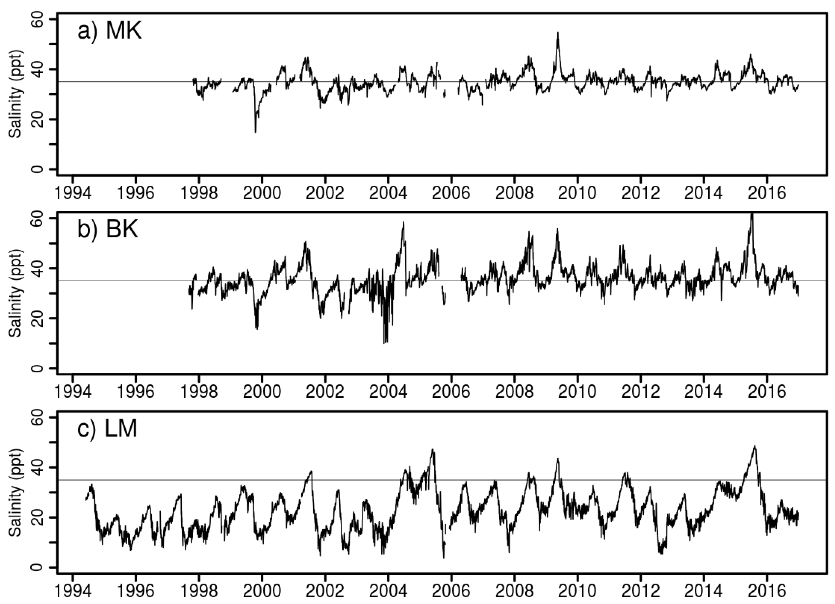
Table 6, we list the change in water level exceedances per year at elevation thresholds above the 90th percentile mean water levels in 1995. Here, we see that in the marine portion of Florida Bay at Murray Key (MK), high-water level exceedances have increased from 2–17% of the days per year over the last two decades, while along the coastal margins, these exceedances have changed from a twice-monthly occurrence, likely at the spring tides, to a nearly every-other-day occurrence.
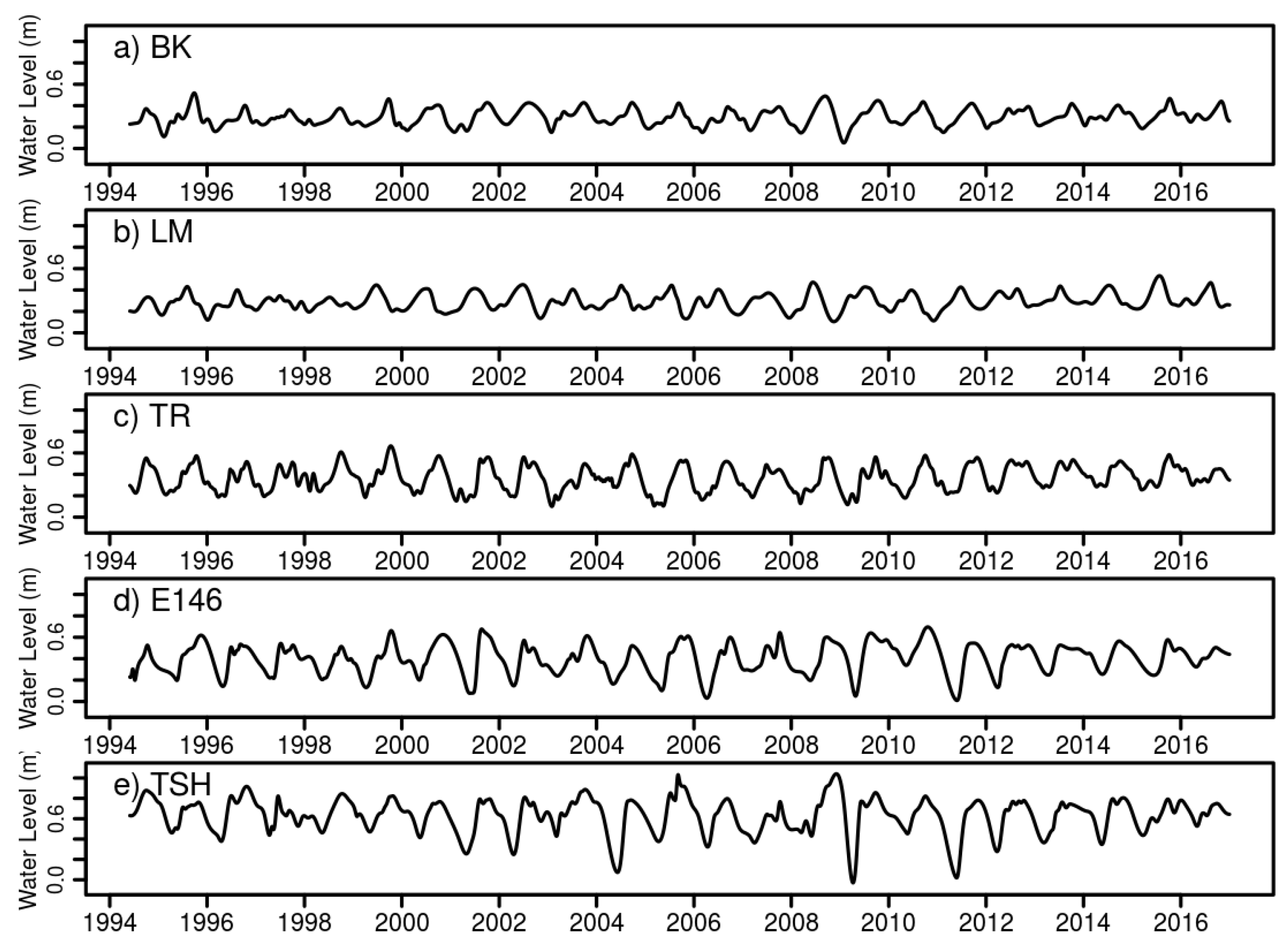
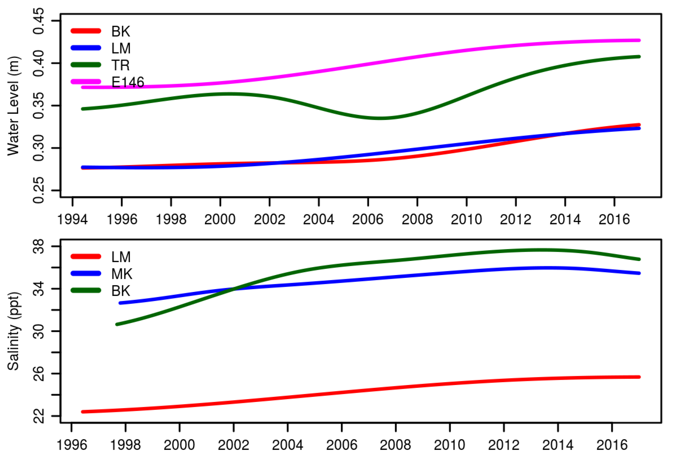
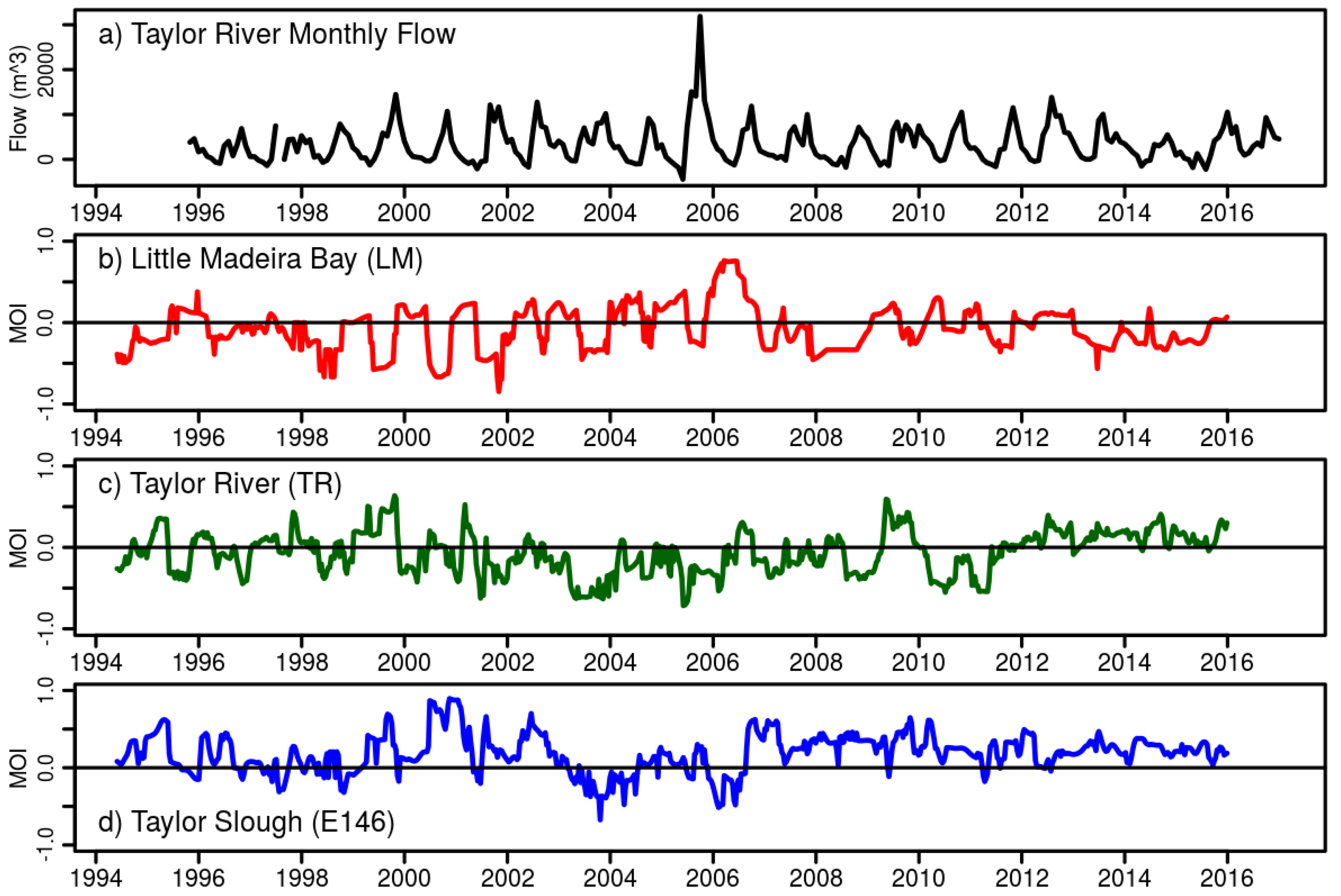
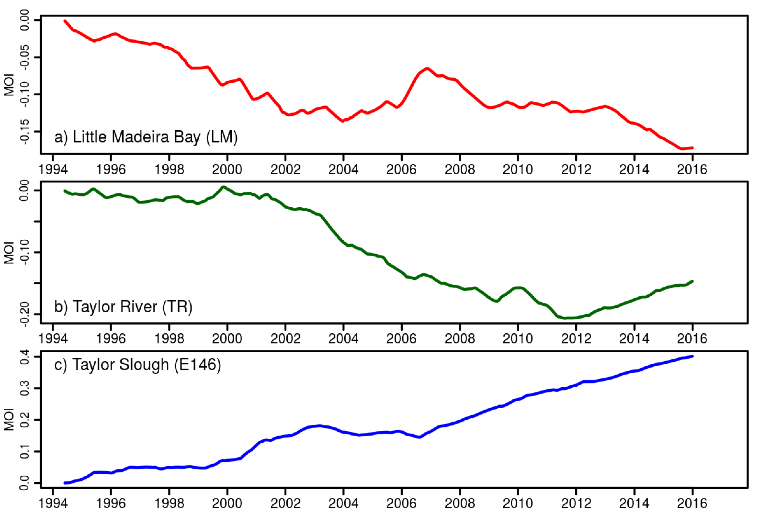
Questions regarding the spatial progression of sea level rise impacts have been addressed with inundation and exceedance projections; however, the presence of hydrographic records spanning the marine-to-freshwater interface provides an opportunity to identify spatially-explicit time series revealing a dynamic transition of water levels from marsh to ocean-dominated. This motivates us to introduce the Marsh-to-Ocean transformation Index (MOI) as a metric to quantify these changes. We find that since 1994, there is a cumulative increase in ocean-dominated hydrographic signals in Little Madeira Bay (LM), as well in the lower reach of Taylor Slough (TR). Farther upstream at station E146, there is no cumulative evidence of ocean influence.

5. Conclusions

Collectively, the data and analysis present a cohesive picture that South Florida landscapes and ecosystems are experiencing a transformation of coastal environments into marine-dominated conditions. Such a transformation will accrue benefits for marine biomes, while decreasing the productivity of coastal freshwater aquifers and presenting challenges for existent freshwater habitats, as well as human infrastructure and habitation.
It is important to note that these projections are for mean sea level and do not consider inundation due to tides or storms. Impacts from tidal inundation will first be noticed at spring tides and then from daily high tides several years or even a decade prior to mean sea level effects. These events will provide opportunities to study the impacts and responses of increasingly frequent inundation events prior to the transformation of existent coastal fringes and freshwater ecosystems into marine-dominated areas. Further, the projections do not incorporate contributions in the event of Antarctic ice-sheet collapse or from changes in ocean circulation and the Florida Current, which have the potential to increase sea levels and compress the forecast time horizons. Regardless of the specific sea level rise trajectory, restoration of the Everglades with increased freshwater flow and water levels will serve to mitigate the impacts of sea level rise over the next century and protect freshwater resources for both the natural and human inhabitants.

Supplementary Materials

GIS coverages of the sea level rise projections are available online at Park and Stabenau [34].

Acknowledgments

The authors are indebted to Caryl Alarcón for expert GIS analysis and support.

Author Contributions

Joseph Park and Erik Stabenau created the sea level rise projection and edited the manuscript. Joseph Park performed the exceedance analysis and suggested and computed the MOI. Jed Redwine edited the manuscript. Kevin Kotun managed the data network and edited the manuscript.

Conflicts of Interest

The authors declare no conflict of interest.

Abbreviations

The following abbreviations are used in this manuscript:
EMDEmpirical Mode Decomposition
IEAInternational Energy Agency
IMFIntrinsic Mode Function
IPCCIntergovernmental Panel on Climate Change
MHHWMean High-Higher Water
MLLWMean Low-Lower Water
MOIMarsh-to-Ocean Index
MSLMean Sea Level
NAVD88North American Vertical Datum of 1988
NGVD29National Geodetic Vertical Datum of 1929
NTDENational Tidal Datum Epoch
RESRenewable Energy Source
RCPRepresentative Concentration Pathway
UNESCOUnited Nations Educational, Scientific and Cultural Organization
USGSUnited States Geological Survey

Appendix A. Datum and Water Level Conversions

A tidal datum [35] provides a geodetic link between ocean water level and a land-based elevation reference such as the North American Vertical Datum of 1988 (NAVD88). The National Tidal Datum Epoch (NTDE) in the United States is a 19-year period over which tidal datums specific to each tide gauge are determined. The current NTDE for the United States is 1983–2001, and sea level rise projections are referenced to the midpoint of this period (1992) consistent with design procedures determined by the U.S. Army Corps of Engineers and NOAA’s National Climate Assessment [36]. Common tidal datums include Mean Sea Level (MSL), Mean High-Higher Water (MHHW) and Mean Low-Lower Water (MLLW), as defined by the National Oceanic and Atmospheric Administration [35]. As sea level rises, tidal datum elevations also, rise and a new tidal datum is established every 20–25 years to account for sea level change and vertical adjustment of the local landmass [37].
Kopp et al. [9] assumed a water level reference of mean sea level starting at year 2000; however, the mean sea level datum at the Vaca Key tide gauge, which can be referenced to NAVD88, is with respect to the National Tidal Datum Epoch (NTDE) centered on 1992. To reference the Kopp projection to NAVD88, we must first account for sea level rise at the tide gauge from 1992–2000. We quantified this sea level rise at Vaca Key with an empirical mode decomposition resulting in value of 1.4 cm. This sea level rise offset is added to the Kopp projections to account for the fact that their projections start in the year 2000, but that the NTDE mean sea level at Vaca Key is referenced to 1992.
Next, we convert the projections with respect to the NTDE mean sea level datum to the NAVD88 geodetic datum of the topographic elevations. Table A1 lists the NTDE and NAVD88 elevations at the Vaca Key tide gauge [38], where we find that the NAVD88 datum is 25.1 cm above the NTDE MSL datum. In other words: MSL referenced to NAVD88 is equal to the NAVD88 datum elevation minus 25.1 cm. We therefore subtract 25.1 cm from all projected water levels with respect to mean sea level in order to reference them to the NAVD88 datum.
Table A1. Elevations on station datum in meters at Vaca Key, FL (NOAA station: 8723970). Tidal datum epoch: 1983–2001.
DatumValueDescription
NAVD881.182North American Vertical Datum of 1988
MHHW1.072Mean Higher-High Water
MHW1.040Mean High Water
MSL0.931Mean Sea Level
MLW0.822Mean Low Water
MLLW0.775Mean Lower-Low Water
STND0.000Station Datum
Finally, we apply the sea level rise projections with respect to NAVD88 to current mean sea level, which is not at zero elevation NAVD88. As above, we note that the NTDE (1992) mean sea level at Vaca Key is −25.1 cm NAVD88, while the current sea level in Florida Bay averaged over 2008–2015 is −14.8 cm NAVD88 (Appendix C). The difference of 10.3 cm reflects sea level rise from 1992–2015 and any local influences of dynamic height between Vaca Key and the three stations where mean sea level was estimated.
Putting this all together, the elevation of −14.8 cm NAVD88 is the starting elevation of the sea level projections, as shown in Figure 2 and Appendix B. The projections from Kopp et al. [9], which have been converted to NAVD88, are then added to this base sea level elevation to predict future mean sea level in Florida Bay.
The cautious reader might consider that there has been a double accounting of sea level rise, 1.4 cm representing the change from 1992–2000 and 10.3 cm for sea level rise from 1992–2015. However, these are two independent adjustments. The 1.4-cm adjustment was solely for the purpose of referencing the Kopp projections to the mean sea level datum (NTDE), which was then referenced to NAVD88, a datum conversion independent of the projection starting time. The 10.3-cm accounts for the fact that we choose 2015 as the starting point of the projections. Had we selected year 2000 as the starting point, then the 1.4 cm datum conversion would still apply, while the adjustment to a starting sea level of 2000 would be less than the 10.3 cm determined for a 2015 start time.

Appendix B. Tabulated Sea Level Rise Projection

Sea level rise in cm NAVD88 from Kopp et al. [9] at Vaca Key. Values between decades (2010, 2020, etc.) have been interpolated with a cubic spline. Low is the 50th percentile of the RCP 8.5 projection; high the 99th percentile. An offset of 1.4 cm has been added to account for sea level rise from 1992–2000 to convert the Kopp projections starting in 2000 to the NTDE MSL datum of 1992. The NAVD88 datum is 25.3 cm above the NTDE MSL, so that 25.3 cm has been subtracted to convert NTDE MSL to NAVD88. The projections have been offset to match observed mean sea level over the period 2008–2015 in Florida Bay of −14.8 cm NAVD88 (Appendix C).
Table A2. Sea level rise in cm NAVD88 from Kopp et al. [9].
YearLowHighYearLowHighYearLowHighYearLowHigh
2015−14.8−14.820456.818207535.876.6210568.3159.9
2016−14.2−13.820467.719.6207636.979210669.5162.7
2017−13.6−12.820478.621.120773881.5210770.8165.4
2018−12.9−11.820489.622.8207839.284210872168.3
2019−12.3−10.8204910.524.4207940.386.5210973.2171.2
2020−11.6−9.8205011.426.2208041.489.2211074.4174.2
2021−10.9−8.9205112.327.9208142.691.8211175.6177.2
2022−10.2−7.9205213.229.7208243.794.5211276.7180.3
2023−9.5−6.9205314.131.6208344.897.2211377.9183.5
2024−8.8−5.920541533.5208445.9100211479186.8
2025−8.1−4.9205515.935.4208547.1102.8211580.1190.1
2026−7.4−3.9205616.837.3208648.2105.6211681.2193.4
2027−6.7−2.9205717.739.3208749.3108.5211782.2196.8
2028−6−1.9205818.641.2208850.3111.3211883.3200.2
2029−5.3−0.9205919.543.2208951.4114.2211984.4203.7
2030−4.60.2206020.445.2209052.4117.2212085.4207.2
2031−3.91.2206121.447.1209153.4120.1
2032−3.22.2206222.349209254.4123
2033−2.63.2206323.351209355.4125.9
2034−1.94.3206424.352.9209456.3128.9
2035−1.25.3206525.354.9209557.3131.8
2036−0.56.4206626.356.9209658.3134.7
20370.27.6206727.358.9209759.3137.6
20380.98.7206828.360.9209860.3140.5
20391.69.9206929.463209961.3143.3
20402.411.2207030.465.2210062.4146.2
20413.212.4207131.567.3210163.5148.9
20424.113.8207232.669.6210264.7151.7
2043515.1207333.671.8210365.9154.4
20445.916.6207434.774.2210467.1157.1

Appendix C. Mean Sea Level in Florida Bay

MSL was determined by averaging data over the last seven years at three sea level stations across Florida Bay. Sea levels were first aggregated into daily averages, followed by a 30-day moving average at each station. The MSL estimate consists of an average of these three stations from 1 July 2008–1 July 2015, as shown in Figure A1, and this MSL value of 0.97 ft NGVD29 or −14.8 cm NAVD88 (−0.49 feet NAVD88) is used as the starting point of the projections in 2015.
Figure A1. Thirty-day moving averages of daily mean sea level at Murray Key (MK), Peterson Key (PK) and Little Madeira Bay (LM) in Florida Bay. The dashed line is the mean of all three datasets.
Jmse 05 00031 g015

Appendix D. Processes Not Included in the Projections

The mean sea level projections presented in this paper represent the contemporary state-of-the-art in local sea level rise forecasts. However, knowledge of all processes and feedbacks driving sea levels is limited, and the models on which these projections are based are necessarily incomplete. The models do not have the spatial resolution and physical process representation required to resolve fine-scale oceanographic processes such as tides and changes in the Florida Current. This means that inundation will be observed during high tides and peaks of seasonal sea level cycles several years before the projected dates when mean sea level reaches a specific land elevation.

Appendix D.1. Tides and Seasonal Cycles

Tides represent the most regular and familiar sea level changes at a coast, but are highly variable in height and timing depending on regional and local bathymetric features. Along the Cape Sable region, tides produce a water level change of up to 70 cm (2.3 ft) in daily and monthly cycles. There is also a regional yearly cycle of water level from atmospheric and oceanographic forcings producing water level changes of 30–40 cm (Appendix C).

Appendix D.2. Florida Current

The Florida Current is one of the strongest and most climatically-important ocean currents forming the headwater of the Gulf Stream [39]. As the Florida Current fluctuates in intensity, sea levels along the Atlantic coast of Florida respond to a geostrophic balance by falling when the current increases and rising when the current decreases [40].
The Gulf Stream and Florida Current are components of the Atlantic Meridional Overturning Circulation (AMOC), a component of the global ocean conveyor belt. Climate models agree that as the ocean warms and fresh meltwater is added, there will be a decline in the strength of the AMOC [41]. A weakening AMOC is expected to result in a weakening of the Florida Current and a subsequent increase in sea levels. The extent of this change is difficult to forecast, but recent evidence suggests that a 10% decline in transport has contributed 60% of the roughly 7-cm increase in sea level at Vaca Key over the last decade [10]. Continued reduction of the AMOC and Florida Current could be expected to contribute an additional 10–15 cm of sea level rise to South Florida over this century. This potential is not reflected in the sea level rise projections, but should be considered by authorities and planners that use them.

Appendix D.3. Storm Surge

Although sea level rise and increases in coastal flooding are important physical stresses on South Florida’s natural areas, it is the infrequent, high-impact storm surge events that drastically change the landscape over the course of a few hours. For example, Hurricane Wilma in 2005 had a profound impact on the ecology of the Cape Sable region of Everglades National Park [42,43] producing extensive damage at the Flamingo Visitor Center of Everglades National Park, permanently closing the Flamingo Lodge and Buttonwood Cafe.
Storm surge is highly dependent on the severity and path of the storm, as well as the local bathymetric and topographic features of the coast, and since they occur infrequently, it is difficult to develop robust predictions of these rare events. A popular approach is to fit an extreme-value probability distribution to the highest water levels observed at a water level monitoring gauge. However, gauges have short periods of record, typically a few decades at most, and they fail or are destroyed during extreme storms such that peak water levels are not recorded. A predictive storm surge database, SurgeDat, was developed in part to address this shortcoming by providing a statistical combination of data from multiple events within an area of interest [44]. SurgeDat records storm surge water levels from all available sources, often from post-event high-water marks where gauge data are not available. SurgeDat then applies a statistical regression to estimate storm surge recurrence intervals. A recurrence interval is the length of time over which one can expect a storm surge to meet or exceed a specific inundation level. A familiar example is the 100-year flood level, which is really a 100-year recurrence interval at the specified flood level. In other words, in any one year, there is a 1/100, or 1% chance that the flood level will be matched or exceeded. An excellent discussion of this can be found at the United States Geological Survey web page water.usgs.gov/edu/100yearflood.html.
Relevant to South Florida, a subset of SurgeDat storm surge events was selected within a 25-mile radius of 25.2° N, 80.7° W to represent Florida Bay impacts and is tabulated in Table A3. Based on these events, the SurgeDat projection for storm surge recurrence intervals are shown in Figure A2 and tabulated in Table A4, suggesting that a 180-cm (6 ft) surge event can be expected every 20 years. This same level of sea level rise is not anticipated to occur until at least 2100.
Table A3. SurgeDat database entries for a 25-mile radius centered on 25.2° N, 80.7° W in Florida Bay.
Storm NameYearLongitudeLatitudeSurge (m)DatumLocation
Katrina2005−81.036925.12941.22ExtremeSW Florida
Rita2005−80.720024.86051.22NGVD29Middle and Upper Keys
Wilma2005−81.035225.35232.50Shark River 3
Gordon1994−80.513925.01081.22Above Sea LevelUpper Florida Keys
Andrew1992−80.912025.14311.50Flamingo
David1979−80.626324.92310.61Above NormalIslamorada
Gladys1968−80.513525.01100.15Above NormalTavernier
Inez1966−80.529724.99761.10Above NormalPlantation Key
Alma1966−80.513525.01100.30Above NormalTavernier
Betsy1965−80.514825.00962.35Mean Low WaterTavernier
Donna1960−80.635324.91334.11Upper Matecumbe Key
Labor Day1935−80.737524.85165.49Lower Matecumbe
Unnamed1929−80.388525.18482.68Mean Sea LevelKey Largo
The recurrence interval projection is by necessity based on a sparse dataset, and caution should be used in its interpretation. As projection intervals become longer, it is more likely that the observed data are inadequate to robustly represent all possibilities. Furthermore, these projections do not incorporate changes from sea level rise or from a changing climate, which can alter the strength and frequency of storms. An important aspect of sea level rise is that it significantly shortens the expected recurrence intervals of storm surge. For example, under a median sea level rise projection at Key West, Park et al. [45] find that a one-in-50-year storm surge based on historic data in 2010 can be expected to occur once every five years by 2060.
Figure A2. Storm surge recurrence intervals from the SurgeDat database and return period predictor for a 25-mile radius centered on 25.2° N, 80.7° W.
Jmse 05 00031 g016
Table A4. Recurrence interval projection in years from the Florida Bay SurgeDat data. Note that this projection does not take into account future sea level rise.
Interval (Year)Surge (m)Interval (Year)Surge (m)
100.45563.88
120.82583.95
141.12604.02
161.39624.08
181.62644.15
201.83664.21
222.02684.27
242.19704.33
262.35724.38
282.50744.44
302.64764.49
322.77784.54
342.89804.59
363.00824.64
383.11844.69
403.21864.73
423.31884.78
443.40904.82
463.49924.87
483.57944.91
503.65964.95
523.73984.99
543.811005.03

References

  1. Cazenave, A.; Le Cozannet, G. Sea level rise and its coastal impacts. Earth’s Future 2013, 2, 15–34. [Google Scholar] [CrossRef]
  2. Light, S.S.; Dineen, J.W. Water control in the Everglades: A historical perspective. In Everglades: The Ecosystem and its Restoration; Davis, S.M., Ogden, J.C., Park, W.A., Eds.; St. Lucie Press: Delray Beach, FL, USA, 1994; p. 826. ISBN 0963403028. [Google Scholar]
  3. National Research Council (NRC). Progress toward Restoring the Everglades: The Fifth Biennial Review—2014; Committee on Independent Scientific Review of Everglades Restoration Progress; Water Science and Technology Board; Board on Environmental Studies and Toxicology; Division on Earth and Life Studies; National Research Council: Washington, DC, USA, 2014; p. 320. Available online: http://www.nap.edu/catalog.php?record_id=18809 (accessed on 25 July 2017). [CrossRef]
  4. Southeast Florida Regional Climate Change Compact (RCCC). A Region Responds to a Changing Climate Southeast Florida Regional Climate Change Compact Counties, Regional Climate Action Plan; October 2012; p. 84. Available online: https://southeastfloridaclimatecompact.files.wordpress.com/2014/05/regional-climate-action-plan-final-ada-compliant.pdf (accessed on 25 July 2017).
  5. Southeast Florida Regional Climate Change Compact (RCCC). The Sea Level Rise Task Force; 2013. Available online: http://www.miamidade.gov/planning/boards-sea-level-rise.asp (accessed on 25 July 2017).
  6. Holland, P.R.; Brisbourne, A.; Corr, H.F.J.; McGrath, D.; Purdon, K.; Paden, J.; Fricker, H.A.; Paolo, F.S.; Fleming, A.H. Oceanic and atmospheric forcing of Larsen C Ice-Shelf thinning. Cryosphere 2015, 9, 1005–1024. [Google Scholar] [CrossRef] [Green Version]
  7. Wouters, B.; Martin-Español, A.; Helm, V.; Flament, T.; van Wessem, J.M.; Ligtenberg, S.R.M.; van den Broeke, M.R.; Bamber, J.L. Dynamic thinning of glaciers on the Southern Antarctic Peninsula. Science 2015, 348, 899–903. [Google Scholar] [CrossRef] [PubMed]
  8. The Intergovernmental Panel on Climate Change (IPCC). Climate Change 2013: The Physical Science Basis; Contribution of Working Group I to the Fifth Assessment Report of the Intergovernmental Panel on Climate Change; 5th Assessment report; Stocker, T.F., Qin, D., Plattner, G.-K., Tignor, M., Allen, S.K., Boschung, J., Nauels, A., Xia, Y., Bex, V., Midgley, P.M., Eds.; Cambridge University Press: Cambridge, UK; New York, NY, USA, 2013. [Google Scholar]
  9. Kopp, R.W.; Horton, R.M.; Little, C.M.; Mitrovica, J.X.; Oppenheimer, M.; Rasmussen, D.J.; Strauss, B.H.; Tebaldi, C. Probabilistic 21st and 22nd century sea-level projections at a global network of tide gauge sites. Earth’s Future 2014, 2, 383–406. [Google Scholar] [CrossRef]
  10. Park, J.; Sweet, W. Accelerated sea level rise and Florida Current transport. Ocean Sci. 2015, 11, 607–615. [Google Scholar] [CrossRef]
  11. National Oceanic and Atmospheric Administration (NOAA). Earth Systems Research Laboratory, CO2 Annual Mean Growth Rate for Mauna Loa, Hawaii; 2017. Available online: https://www.esrl.noaa.gov/gmd/ccgg/trends/gr.html (accessed on 25 July 2017).
  12. Jones, G.A.; Warner, K.J. The 21st century population-energy-climate nexus. Energy Policy 2016, 93, 206–212. [Google Scholar] [CrossRef]
  13. International Energy Agency. Medium-Term Renewable Energy Market Report 2016; Available online: https://www.iea.org/newsroom/news/2016/october/medium-term-renewable-energy-market-report-2016.html (accessed on 25 July 2017).
  14. United Nations REN21. Renewables 2016 Global Status Report (Paris: REN21 Secretariat); ISBN 978-3-9818107-0-7. 2016; Available online: www.ren21.net/status-of-renewables/global-status-report/ (accessed on 25 July 2017).
  15. DeConto, R.M.; Pollard, D. Contribution of Antarctica to past and future sea-level rise. Nature 2016, 531, 591–597. [Google Scholar] [CrossRef] [PubMed]
  16. Fennema, R.; James, F.; Bhatt, T.; Mullins, T.; Alarcon, C. EVER Elevation (Version 1): A Multi-Sourced Digital Elevation Model for Everglades National Park; National Park Service: Homestead, FL, USA, 2015. [Google Scholar]
  17. Lentz, E.; Thieler, E.; Plant, N.; Stippa, S.; Horton, R.; Gesch, D. Evaluation of dynamic coastal response to sea-level rise modifies inundation likelihood. Nat. Clim. Chang. 2016, 6, 696–700. [Google Scholar] [CrossRef]
  18. Passeri, D.L.; Hagen, S.C.; Medeiros, S.C.; Bilskie, M.V.; Alizad, K.; Wang, D. The dynamic effects of sea level rise on low-gradient coastal landscapes: A review. Earth’s Future 2015, 3, 159–181. [Google Scholar] [CrossRef]
  19. United Nations Educational, Scientific, and Cultural Organization (UNESCO). The Practical Salinity Scale 1978 and the International Equation of State of Seawater 1980; Unesco Technical Papers in Marine Science 36, 1981; Available online: http://unesdoc.unesco.org/images/0004/000461/046148eb.pdf (accessed on 25 July 2017).
  20. Huang, N.E.; Wu, Z. A review on Hilbert-Huang transform: Method and its applications to geophysical studies. Rev. Geophys. 2008, 46, RG2006. [Google Scholar] [CrossRef]
  21. Chambers, D.P. Evaluation of empirical mode decomposition for quantifying multi-decadal variations and acceleration in sea level records. Nonlin. Process. Geophys. 2015, 22, 157–166. [Google Scholar] [CrossRef]
  22. Sweet, W.; Park, J. From the extreme to the mean: Acceleration and tipping points of coastal inundation from sea level rise. Earth’s Future 2014, 2, 579–600. [Google Scholar] [CrossRef]
  23. Akaike, H. A new look at the statistical model identification. IEEE Trans. Autom. Control 1974, 19, 716–723. [Google Scholar] [CrossRef]
  24. USGS. Measuring and Mapping the Topography of the Florida Everglades for Ecosystem Restoration; FS-021-03; March 2003. Available online: https://sofia.usgs.gov/publications/fs/021-03/factsheet02103-Desmond.pdf (accessed on 25 July 2017).
  25. Byrd, R.H.; Lu, P.; Nocedal, J.; Zhu, C. A limited memory algorithm or bound constrained optimization. SIAM J. Sci. Comput. 1995, 16, 1190–1208. [Google Scholar] [CrossRef]
  26. Ross, M.S.; Gaiser, E.E.; Meeder, J.F.; Lewin, M.T. Multi–Taxon Analysis of the “White Zone”, a Common Ecotonal Feature of South Florida Coastal Wetlands. In Linkages Between Ecosystems in the South Florida Hydroscape: The River of Grass Continues; CRC Press: Boca Raton, FL, USA, 2001; pp. 205–238. [Google Scholar]
  27. Dausman, A.; Langevin, C.D. Movement of the Saltwater Interface in the Surficial Aquifer System in Response to Hydrologic Stresses and Water-Management Practices, Broward County, Florida; USGS Scientific Investigations Report 2004-5256; 2005. Available online: http://pubs.usgs.gov/sir/2004/5256/ (accessed on 25 July 2017).
  28. Hanson, S.; Nicholls, R.; Ranger, N.; Hallegatte, S.; Corfee-Morlot, J.; Herweijer, C.; Chateau, J. A global ranking of port cities with high exposure to climate extremes. Clim. Chang. 2011, 104, 89–111. [Google Scholar] [CrossRef] [Green Version]
  29. Hutchison, J.; Manica, A.; Swetnam, R.; Balmford, A.; Spalding, M. Predicting Global Patterns in Mangrove Forest Biomass. Conserv. Lett. 2014, 7, 233–240. [Google Scholar] [CrossRef]
  30. Wanless, H.; Parkinson, R.; Tedesco, L. Sea level control on stability of Everglades wetlands. In Everglades: The Ecosystem and Its Restoration; Davis, S.M., Ogden, J.C., Eds.; St. Lucie Press: Delray Beach, FL, USA, 1997; pp. 199–223. [Google Scholar]
  31. National Aeronautic and Space Administration (NASA). Sea Level Change, Observations from Space; 2017. Available online: https://sealevel.nasa.gov/ (accessed on 10 July 2017).
  32. Fuller, D.O.; Wang, Y. Recent Trends in Satellite Vegetation Index Observations Indicate Decreasing Vegetation Biomass in the Southeastern Saline Everglades Wetlands. Wetlands 2014, 34, 67–77. [Google Scholar] [CrossRef]
  33. Doyle, T.W. Predicting Future Mangrove Forest Migration in the Everglades under Rising Sea Level; USGS Fact Sheet FS-030-03; U.S. Department of the Interior; U.S. Geological Survey, March 2003. Available online: https://www.nwrc.usgs.gov/factshts/030-03.pdf (accessed on 25 July 2017).
  34. Park, J.; Stabenau, E. South Florida sea level rise projections. U.S. Department of Interior; National Park Service; South Florida Natural Resources Center: Homestead, Florida, USA, High projection: http://nps.maps.arcgis.com/home/webmap/viewer.html?layers=b61db3e154104ea486528c031390066c. Low projection: http://nps.maps.arcgis.com/home/webmap/viewer.html?layers=87e87e094680431eab085a18adb36836; (accessed on 27 July 2017).
  35. National Oceanic and Atmospheric Administration (NOAA). Tidal Datums; 2016. Available online: http://tidesandcurrents.noaa.gov/datum_options.html (accessed on 25 July 2017).
  36. US Army Corps of Engineers (USACE). Procedures to Evaluate Sea Level Change: Impacts, Responses and Adaptation; U.S. Army Corps of Engineers: Washington, DC, USA; Technical Letter No. 1100-2-1; 30 June 2014. Available online: http://www.publications.usace.army.mil/Portals/76/Publications/EngineerTechnicalLetters/ETL_1100-2-1.pdf (accessed on 25 July 2017).
  37. National Oceanic and Atmospheric Administration (NOAA). Tidal Datums and Their Applications, Special Publication NOS CO-OPS 1; National Oceanic and Atmospheric Administration; National Ocean Service Center for Operational Oceanographic Products and Services, 2001; p. 111. Available online: http://tidesandcurrents.noaa.gov/publications/tidal_datums_and_their_applications.pdf (accessed on 25 July 2017).
  38. National Oceanic and Atmospheric Administration (NOAA). Vaca Key Tidal Datums; 2016. Available online: http://tidesandcurrents.noaa.gov/datums.html?id=8723970 (accessed on 25 July 2017).
  39. Gyory, J.; Rowe, E.; Mariano, A.; Ryan, E. The Florida Current; Ocean Surface Currents; The Rosenstiel School of Marine and Atmospheric Science, University of Miami, 1992; Available online: http://oceancurrents.rsmas.miami.edu/atlantic/florida.html (accessed on 25 July 2017).
  40. Montgomery, R.B. Fluctuations in Monthly Sea Level on Eastern U. S. Coast as Related to Dynamics of Western North Atlantic Ocean. J. Mar. Res. 1938, 1, 165–185. [Google Scholar] [CrossRef]
  41. Rahmstorf, S.; Box, J.; Feulner, G.; Mann, M.; Robinson, A.; Rutherford, S.; Schaffernicht, E. Exceptional twentieth-century slowdown in Atlantic Ocean overturning circulation. Nat. Clim. Chang. 2015, 5, 475–480. [Google Scholar] [CrossRef] [Green Version]
  42. Smith, T.J., III; Anderson, G.H.; Balentine, K.; Tiling, G.; Ward, G.A.; Whelan, K.R.T. Cumulative Impacts of Hurricanes on Florida Mangrove Ecosystems: Sediment Deposition, Storm Surges and Vegetation. Wetlands 2009, 29, 24–34. [Google Scholar] [CrossRef]
  43. Whelan, K.R.T.; Smith, T.J.; Anderson, G.H.; Ouellette, M.L. Hurricane Wilma’s impact on overall soil elevation and zones within the soil profile in a mangrove forest. Wetlands 2009, 29, 16–23. [Google Scholar] [CrossRef]
  44. Needham, H.F.; Keim, B.D.; Satharaj, D.; Shafer, M. A Global Database of Tropical Storm Surges. EOS Trans. 2013, 94, 213–214. [Google Scholar] [CrossRef]
  45. Park, J.; Obeysekera, J.; Irizarry, M.; Trimble, P. Storm Surge Projections and Implications for Water Management in South Florida. Clim. Chang. 2011, 107, 109–128. [Google Scholar] [CrossRef]
1.
The number following RCP quantifies the expected thermodynamic radiative forcing relative to pre-industrial values. For example, RCP 8.5 denotes an additional 8.5 W / m 2 thermal forcing from greenhouse gases.
2.
Ignoring the nonlinear nature of these trends, one might consider a linear mean water level rise of 5 cm/21 years = 2.4 mm/year, a result coincident with linear estimates of mean sea level rise over the 20th Century; however, examination of the BK data found an increase over the last decade of 4.0 cm, suggesting a recent rate of 4 mm/year, a value somewhat larger than current global estimates of 3.4 mm/year (https://sealevel.nasa.gov/) and an illustration of difficulties in applying linear metrics to nonlinear processes.
Figure 1. Physiographic map of South Florida representing different ecological domains dictated by topography, hydrology and climate. Hydrographic stations are denoted with abbreviations; for example, LM for Little Madeira Bay (Table 1). Everglades National Park (green border) covers the majority of the region with coastal hydrographic stations in Florida Bay (MK, BK, LM, LS, MD) and extending upstream to Taylor Slough (TR, E146, TSH). Urban, suburban and agricultural lands featuring water management canal infrastructure can be seen between Everglades and Biscayne National Parks (blue border).
Jmse 05 00031 g001
Figure 2. South Florida sea level rise projection with respect to 2015 mean sea level in Florida Bay for the RCP 8.5 greenhouse gas emission scenario. Units are cm NAVD88. Low projection is the median (50th percentile); high projection the 99th percentile. Tides and storm surges are not included in this projection. Values are tabulated in Appendix B to year 2120.
Jmse 05 00031 g002
Figure 3. Daily mean water level with respect to the National Geodetic Vertical Datum of 1929 (NGVD29) at 5 stations in Florida Bay and the southern Everglades. Stations BK (a) and LM (b) are in Florida Bay; stations TR (c), E146 (d) and TSH (e) are within Taylor Slough.
Jmse 05 00031 g003
Figure 4. Daily mean salinity at 3 stations in Florida Bay. The horizontal line at 35 ppt represents nominal seawater salinity. (a) MK; (b) BK; (c) LM.
Jmse 05 00031 g004
Figure 5. Low frequency cumulative IMFs of water level data in Florida Bay and Taylor Slough shown in Figure 3. (a) BK; (b) LM; (c) TR; (d) E146; (e) TSH.
Jmse 05 00031 g005
Figure 6. Low frequency IMFs at the BK and TSH stations to represent ocean-dominated and marsh-dominated hydrologic dynamics respectively. (a) Intra-annual modes; (b) annual modes; (c) comparison of low pass water level signals at BK and TSH constructed from the addition of the IMFs in (a) and (b).
Jmse 05 00031 g006
Figure 7. Mean sea level elevation maps for South Florida including Everglades and Biscayne National parks for the median (50th) and high (99th percentile) RCP 8.5 projections using current topography and the NAVD88 datum. Tides and storm surges are not included in this projection.
Jmse 05 00031 g007
Figure 8. Mean sea level elevation maps for Dry Tortugas National Park at Loggerhead, Garden, Bush and Long Keys for the median (50th) and high (99th percentile) RCP 8.5 projections. Tides and storm surges are not included in this projection.
Jmse 05 00031 g008
Figure 9. Sea level rise inundation maps at Flamingo in Everglades National Park (top row) and Fort Jefferson in Dry Tortugas National Park (bottom row). Building and infrastructure footprints are indicated in red.
Jmse 05 00031 g009
Figure 10. Yearly water level elevation exceedance data and fits to the model of Equation (1). Elevation thresholds are with respect to the NGVD29 datum. Note that the MD station is located on a higher land elevation than the other three stations. (a) MK; (b) LM; (c) LS; (d) MD.
Jmse 05 00031 g010
Figure 11. Projected evolution of water level exceedances at Little Madeira Bay under the low and high sea level rise scenarios. Mean water is the daily mean water level over the three-year period from January 2014–December 2016.
Jmse 05 00031 g011
Figure 12. Nonlinear trends of water level and salinity at hydrographic stations in Florida Bay and Taylor Slough.
Jmse 05 00031 g012
Figure 13. (a) Monthly stream flow at the terminus of Taylor River; (b) Marsh-to-Ocean Index (MOI) in Little Madeira Bay (LM) over a one year-long moving window advanced in 10-day increments; (c) MOI at the Taylor River (TR) station; (d) MOI at the E146 station in Taylor Slough.
Jmse 05 00031 g013
Figure 14. Integral over time of the Marsh-to-Ocean Index (MOI) at: (a) Little Madeira Bay (LM); (b) Taylor River (TR); and (c) Taylor Slough (E146).
Jmse 05 00031 g014
Table 1. Hydrographic stations.
StationLocationLatitudeLongitudeWater LevelSalinity
BKBuoy Key25.12111−80.83356WaterLog H-331YSI 600R
E146Taylor Slough25.25252−80.66626WaterLog H-331
LMLittle Madeira Bay25.17580−80.63269WaterLog H-331YSI 600R
LSLong Sound25.23516−80.45680WaterLog H-331YSI 600R
MDSouth Dade25.28932−80.39642WaterLog H-331YSI 600R
MKMurray Key25.10613−80.94232WaterLog H-331YSI 600R
TRTaylor River25.21712−80.64957WaterLog H-331YSI 600R
TSHTaylor Slough Hilton25.31073−80.63100WaterLog H-331
Table 2. Station time series statistics.
StationLocationWater Level (m) NGVD Salinity (ppt)
minmeanmax σ minmeanmax σ
BKBuoy Key−0.120.291.030.1099.9435.9166.075.70
LMLittle Madeira Bay−0.030.310.890.1103.7022.9248.768.02
TRTaylor River0.080.370.890.125
MKMurray Key−0.510.220.890.12714.6734.8454.793.60
E146Taylor Slough−0.180.390.800.143
TSHTaylor Slough Hilton−0.120.631.020.176
Table 3. Initial values and phase space search increments for the exceedance model parameters of Equation (1).
ParameterValuesIncrement
E 0 10
α 10
T L 1990–20105
T G 1995–20105
r0–20020
τ 0–6020
Table 4. Exceedance model parameters at an elevation threshold of 35 cm NGVD29 at Murray Key (MK), Little Madeira Bay (LM) and Long Sound (LS). Note that the South Dade (MD) station is located on a higher land elevation and uses a threshold of 85 cm NGVD29.
StationThreshold (cm) E 0 α T L T G r τ
Murray Key (MK)3542.382.462005.512007.63381.4010.32
Little Madeira (LM)3571.493.991996.772000.39134.3616.82
Long Sound (LS)3583.801.802008.451998.01229.1020.36
South Dade (MD)8566.552.591998.341992.00208.8726.12
Table 5. Marsh-to-Ocean Index (MOI) values over the period 1 January 2014–31 December 2016 at stations LM, TR and E146 relative to the ocean-dominated station at Buoy Key (BK) and the marsh-dominated station at TSH.
Station ω 1 ω 2 ω 3 Ω μ 1 μ 2 μ 3 MMOI
LM0.000.620.000.620.000.000.000.00−0.21
TR0.460.380.000.840.320.580.000.900.02
E1460.260.000.000.260.410.850.001.260.34
Table 6. Number of days per year of water level exceedance in 1995 and 2015.
StationMKLMLSMD
Threshold40 cm40 cm40 cm90 cm
Year19952015199520151995201519952015
Days661271613413329149
Percent Days217744936841

