Article

An Adaptive Receiver-Grid Parameter Optimization Method for BELLHOP Based on Bathymetric and Sound-Speed-Profile Features


1
College of Ocean Science and Engineering, Shandong University of Science and Technology, Qingdao 266590, China
2
Key Laboratory of Underwater Acoustic Communication and Marine Information Technology (Xiamen University), Ministry of Education, Xiamen 361000, China
3
College of Mechanical and Electronic Engineering, Shandong University of Science and Technology, Qingdao 266590, China
4
College of Geodesy and Geomatics, Shandong University of Science and Technology, Qingdao 266590, China
5
First Institute of Oceanography, Ministry of Natural Resources, Qingdao 266061, China
6
Key Laboratory of Marine Science and Numerical Modeling, Ministry of Natural Resources, Qingdao 266061, China
7
Laboratory for Regional Oceanography and Numerical Modeling, Qingdao Marine Science and Technology Center, Qingdao 266061, China
*
Author to whom correspondence should be addressed.
J. Mar. Sci. Eng. 2026, 14(8), 756; https://doi.org/10.3390/jmse14080756
Submission received: 11 March 2026 / Revised: 9 April 2026 / Accepted: 17 April 2026 / Published: 21 April 2026
(This article belongs to the Special Issue Marine Modelling and Environmental Statistics—2nd Edition)

Highlights

What are the main findings?
  • An adaptive receiver-grid construction method for the BELLHOP model is proposed, in which the horizontal and vertical grid spacings are dynamically adjusted according to the seabed topographic slope and sound-speed-profile gradients, thereby enabling a more effective representation of acoustic-field variations in complex ocean environments.
  • Comparative experiments under seamount, trench, and slope scenarios show that the proposed method reduced computational time and storage cost while maintaining RMSE comparable to that of the 100 × 15 m uniform grid, with advantages in resolving local acoustic-field features in topographically sensitive regions.
What are the implications of the main findings?
  • The proposed adaptive-grid method provides an effective approach for improving the efficiency of acoustic-propagation simulation in complex marine environments, helping to alleviate the trade-off between accuracy, efficiency, and resource consumption encountered in conventional uniform-grid methods.
  • The resulting capability can support high-fidelity acoustic-field modeling, transmission-loss prediction, and performance evaluation under complex topographic conditions, thereby providing a methodological reference for adaptive acoustic simulation in complex marine environments.

Abstract

Ray-based models have been extensively applied in underwater acoustic propagation modeling because of their favorable physical interpretability and engineering practicality. Nevertheless, in complex ocean environments, conventional acoustic propagation models still face several limitations, including low computational efficiency, empirically determined grid settings, and inadequate local refinement capability, which restrict their application in high-accuracy and high-efficiency simulations. To address these limitations, an adaptive receiver-grid construction method for the BELLHOP model is proposed in this study. The method adaptively adjusts receiver-grid spacings by using seafloor bathymetric features and sound-speed-profile gradient characteristics as the primary driving factors. Specifically, local grid refinement is introduced in the receiver-grid region of critical acoustic propagation areas, whereas relatively coarse grids are employed in non-critical regions, thereby improving acoustic-field resolution while reducing the overall computational cost. Simulation results show that the proposed method effectively improves the transmission-loss computation efficiency and spatial resolution of the BELLHOP model in complex ocean environments, thus providing a practical approach for rapid and high-precision underwater acoustic propagation modeling.

1. Introduction

As China’s marine survey and development activities continue to expand from coastal waters toward the deep and open ocean, increasing demands are being placed on the rapid and accurate computation of acoustic fields, as well as on the reliable modeling of underwater acoustic channels for tasks such as underwater detection, communication, and environmental sensing. Ocean acoustic propagation [1,2] is governed jointly by multiple factors, including the sound-speed profile, sea-surface and seabed boundaries, and medium absorption and scattering [3,4,5]. As a result, transmission loss and ray structure exhibit pronounced spatiotemporal inhomogeneity, making acoustic-field prediction inherently complex and uncertain. To address these challenges, several classical approaches to acoustic-field modeling have been developed [6,7]. These include normal-mode models, ray models [8,9,10], wavenumber integration models, parabolic equation models, multipath expansion methods, and efficient acoustic-field approximation methods. Among these, ray theory describes energy propagation paths under high-frequency conditions based on the principles of geometric acoustics, offering intuitive physical interpretability and high computational efficiency. It is particularly suitable for engineering scenarios involving significant horizontal variability or requiring rapid assessment, and has therefore been widely applied in acoustic-field simulation and parameter inversion.
The BELLHOP model, developed by Porter [11] and Bueker, is an acoustic propagation model that employs the Gaussian beam tracing method [12] to calculate acoustic fields in horizontally inhomogeneous environments. BELLHOP is well-suited for solving range-dependent problems involving high-frequency signals and is primarily applied to two-dimensional, horizontally invariant waveguide interfaces. The model mainly outputs information such as channel impulse responses, ray trajectories, and transmission loss. By using the BELLHOP model, it is possible to simulate target echo signals received by hydrophones in deep-sea acoustic fields [13,14]. The extraction and analysis of target motion parameters from these echoes provide the prerequisite for target tracking.
As the demand for acoustic-field simulation in complex environments continues to increase, considerable efforts have been made to improve the computational efficiency of ray-based models, particularly BELLHOP. Existing studies have mainly focused on parallel implementation, workflow optimization, and approximation strategies. Parallel computing frameworks and heterogeneous hardware provide a direct means of accelerating ray tracing and field computation. For example, MPI-based multi-node implementations have significantly improved the speed of BELLHOP simulations [15], while CUDA-based parallelization and multithreading have enabled rapid acoustic-field prediction in BellhopMP [16]. GPU-based approaches have also been explored, such as the use of the Nvidia OptiX ray-tracing engine to simulate underwater acoustic propagation with reduced runtime [17]. However, these methods often rely strongly on specific hardware and software platforms, which limits their generality and portability.
In addition to hardware acceleration, researchers have sought to reduce the computational burden of individual simulations through algorithmic modifications to ray tracing and error control. Representative approaches include GPU-based parallel eigenray computation for multi-source and multi-receiver scenarios [18], backward-error-based fast acoustic-field calculation in the BELLHOPBP model [19], and adaptive unstructured mesh generation for KRAKEN3D using the OMesh2KRAKEN tool [20,21,22]. Other studies have attempted to reduce computational cost by reducing ray numbers and optimizing step sizes [23]. Although these methods improve efficiency to varying degrees, they still present clear limitations: parallel schemes remain dependent on hardware platforms and implementation complexity, whereas simplified strategies such as ray pruning and step-size compression [24,25] may compromise accuracy in complex environments, particularly in the characterization of multipath propagation and local acoustic features. In contrast, adaptive-grid methods [26,27,28] offer a more flexible and potentially more general solution by dynamically allocating discretization density according to environmental complexity and acoustic-field variability. This strategy enables fine representation in critical regions and coarser discretization in smoother regions, thereby reducing computational and storage costs [29,30,31,32,33,34] while maintaining modeling accuracy.
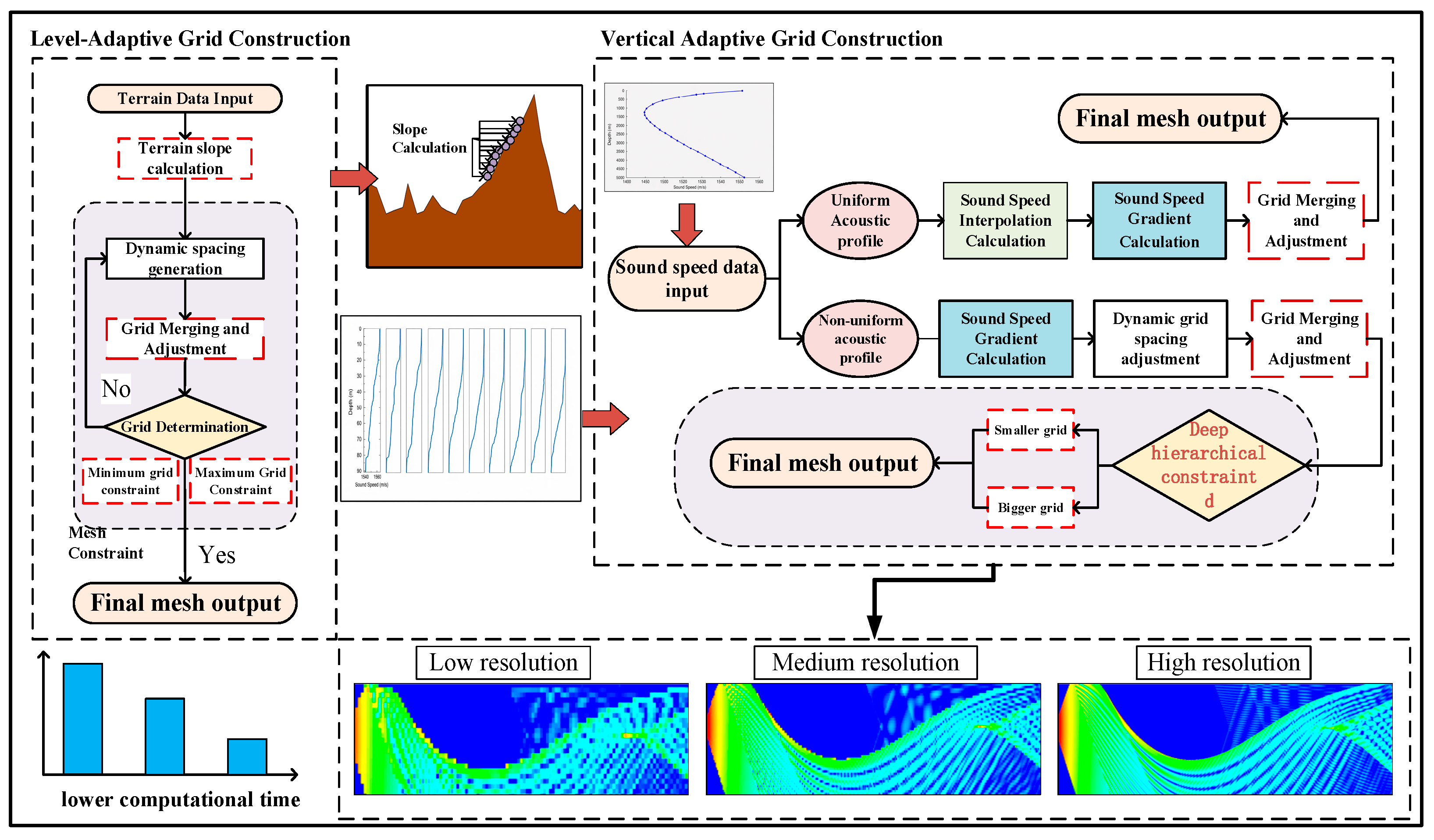
To address the above issues, this study focuses on the computational framework of ocean acoustic ray models and proposes an adaptive grid-parameter optimization method. The overall logical framework of the paper is illustrated in Figure 1. The main contributions are summarized as follows:
  • An adaptive grid-parameter optimization method is proposed for numerical modeling of underwater acoustic propagation. The method adaptively adjusts the receiver-grid resolution of the BELLHOP model according to seabed topography and ocean environmental characteristics, thereby improving computational efficiency while maintaining acoustic-field modeling accuracy and providing a more flexible grid-construction strategy for transmission-loss prediction in complex marine environments.
  • In the simulation part, the proposed adaptive-grid method is validated and analyzed under different ocean acoustic propagation scenarios. The results show that the method can achieve a reasonable allocation of grid resolution according to environmental complexity, effectively reducing computational time and storage cost while maintaining the accuracy of transmission-loss calculations and the ability to represent acoustic-field structures. This demonstrates its effectiveness and potential advantages for fast acoustic-field modeling in complex marine environments.
Figure 1. Overall logical framework of the paper.
Jmse 14 00756 g001

2. Methodology of This Paper

2.1. Ray Acoustics Theory

In the ocean environment, electromagnetic waves experience substantial attenuation in seawater, whereas acoustic waves, due to their relatively low attenuation, serve as the principal carrier for long-range underwater information transmission and detection. Ray acoustics is an approximate approach for modeling underwater acoustic propagation under the framework of geometric acoustics. It provides an intuitive physical interpretation of propagation paths and energy variations, while offering high computational efficiency, and has thus been widely applied in the rapid calculation of ocean acoustic fields. From a mathematical perspective, ray theory represents the high-frequency approximation of wave theory. The standard wave equation can be written as follows:
2 p 1 c 2 2 p t 2 = 0
where p denotes the acoustic pressure, c denotes the sound speed, t is the time variable, and denotes the Hamilton operator.
In the frequency domain, the acoustic pressure field is governed by the Helmholtz equation. For a two-dimensional vertical-section problem with axisymmetric characteristics, described by range r and depth z , the Helmholtz equation can be expressed as follows:
1 r r r p r + q ( z ) z 1 q ( z ) p z + ω 2 c 2 ( z ) p = δ ( r ) δ z z s 2 π r
where p is the complex acoustic pressure, ω is the angular frequency, c is the sound-speed profile, z s is the source depth, and δ is the Dirac delta function.
Transmission loss (TL) is commonly used to describe the spatial attenuation characteristics of an acoustic field. For a given receiver location ( z , r ) , TL is defined in terms of the acoustic pressure amplitude | p ( z , r ) | as follows:
T L ( z , r ) = 20 log 10 | p ( z , r ) |
This metric directly characterizes the attenuation of acoustic energy as a function of range and depth, and constitutes a fundamental output for acoustic-field prediction and performance evaluation. When the acoustic wavelength is much smaller than the characteristic scale of environmental variation, the wave field can be approximated by the geometric-acoustics framework, in which sound propagation is described in terms of ray trajectories and amplitude evolution along the rays.
Under the geometric-acoustics approximation, acoustic energy is assumed to propagate approximately along ray paths. When only the vertical variation in sound speed is considered, the ray trajectories satisfy Snell’s invariant [35]:
p h = sin θ ( z ) c ( z ) = c o n s t
where θ ( z ) denotes the angle between the ray path and the horizontal plane. This relation reveals how sound-speed gradients govern ray refraction and provides the fundamental theoretical basis for ray-based acoustic propagation models.
On this basis, the BELLHOP model, as a representative ray-acoustic tool, numerically traces acoustic ray paths in a range-dependent sound-speed field and incorporates sea-surface and seabed boundary conditions to account for reflection, refraction, and acoustic energy accumulation. As shown in Figure 2, it can effectively predict the acoustic-field distribution, transmission loss, and ray structure within the region of interest. Owing to its clear physical interpretation and high computational efficiency, BELLHOP has been widely used in ocean acoustic modeling and underwater acoustic engineering applications.

2.2. Adaptive Grid Parameter Adjustment Method

In ocean acoustic field simulation, the receiver-grid construction strategy has a significant influence on computational accuracy, efficiency, and storage requirements. Conventional acoustic-field modeling generally employs a fixed-interval grid discretization scheme. While simple and easy to implement, this method cannot effectively balance accuracy and computational cost under complex ocean conditions. In the presence of strong sound-speed gradients or pronounced bathymetric variations, fixed grids may cause oversampling in relatively smooth regions and insufficient resolution in critical areas, thus affecting the reliability of simulation results. A systematic analysis of the relationship between propagation step size and receiver-grid spacing indicates that the suitability of grid discretization directly governs the stability of acoustic energy distribution calculations and the convergence behavior of numerical errors.
To address this issue, an adaptive receiver-grid construction [36] algorithm is proposed by introducing algorithmic improvements to the conventional BELLHOP ray-acoustic model. Through the joint analysis of sound-speed-profile gradients and topographic slopes, the proposed algorithm enables dynamic adjustment of grid spacing, thereby automatically refining the grid in regions with strong acoustic-field variations while moderately coarsening it in relatively smooth regions. Since the receiver grid in the BELLHOP model consists of a horizontal grid (range grid) and a vertical grid (depth grid), which are controlled by different environmental factors, the proposed algorithm treats the two directions separately. In the horizontal direction, grid density is mainly adjusted according to seabed topographic variability and boundary geometry, whereas in the vertical direction, the grid is adaptively layered based on the gradient distribution of the sound-speed profile, thus enabling an optimal trade-off between simulation accuracy and computational efficiency.
The exponential mapping adopted in this study is an empirical, engineering-oriented choice rather than a form derived from rigorous error analysis or theoretical optimality. It was selected because the receiver-grid spacing is expected to vary monotonically with increasing bathymetric slope or sound-speed-profile gradient, while remaining smooth and strictly positive for practical grid construction. In addition, this form can provide stronger local refinement in acoustically or topographically complex regions and milder adjustment in relatively smooth regions. By comparison, linear mapping may lead to abrupt spacing variations, whereas logarithmic mapping generally exhibits weaker sensitivity for local refinement.

2.2.1. Construction of the Horizontal Adaptive Grid

During sound propagation, complex seabed topography may induce reflection, scattering, and diffraction effects. A slope-based adaptive grid achieves demand-driven allocation of discretization resolution by locally refining the grid in regions with significant topographic variations and moderately coarsening it in relatively smooth regions. This strategy reduces computational cost and improves overall computational efficiency while maintaining simulation accuracy.
Topographic Slope Calculation
The BELLHOP bathymetry file (.bty) is imported to obtain the seabed depth points and their corresponding horizontal coordinates. To mitigate the effect of isolated outliers on slope estimation, the original depth sequence is first smoothed to obtain a refined depth profile. The topographic slope [37] is then calculated using a central-difference scheme at interior nodes, whereas forward and backward difference schemes are adopted at the two boundaries, as expressed in Equation (5). The absolute slope at each horizontal position is subsequently used to quantify the local degree of topographic variation.
S i = z i + 1 z i 1 2 Δ x
where S i is the absolute topographic slope at the i horizontal location, z i 1 and z i + 1 are the seabed depths at the two neighboring nodes, and Δ x denotes the mean horizontal spacing between adjacent topographic nodes. At the boundary points, the slope is evaluated using forward- and backward-difference schemes, as given by
S 1 = z 2 z 1 Δ x
S N = z N z N 1 Δ x
Dynamic Adjustment of Grid-Node Spacing Based on Topographic Slope
As the topographic slope increases, acoustic propagation paths in that region become more susceptible to refraction and multiple reflections, thereby requiring higher grid resolution. To allow the grid density to vary adaptively with slope, a sensitivity coefficient is introduced to map the topographic slope to the corresponding target grid spacing. Specifically, after the minimum and maximum horizontal grid spacings are prescribed in advance, an exponential mapping function is used to convert slope values into local grid spacing, as given in Equation (8).
Δ x i = Δ x max 1 + α S i Δ x min Δ x i Δ x max
where Δ x i is the horizontal grid spacing at the i grid node, and Δ x max and Δ x min denote the allowable maximum and minimum horizontal grid spacings. α is a sensitivity coefficient, set to 100 in this study based on repeated experimental optimization. It controls the influence of topographic slope on horizontal grid spacing. The sensitivity coefficient α was determined through experimental optimization. To clarify the basis for its selection, a parameter sensitivity analysis was further conducted using representative bathymetric data, and the effects of different α values on model runtime and acoustic-field error were compared, where the error was quantified by the RMSE relative to the fine-grid reference solution. The specific results are shown in Table 1. The results show that when α is small, the regulating effect of bathymetric slope on horizontal grid spacing is weak, resulting in insufficient local refinement in complex terrain regions and relatively large RMSE values. As α increases, local refinement in complex regions becomes more sufficient, and the error decreases accordingly. In the present test, when α increased from 10 to 100, the RMSE decreased from 2.64 Pa to 1.51 Pa, while the runtime increased only from 3.2 s to 4.4 s, indicating that a noticeable improvement in accuracy can be achieved within this range at an acceptable computational cost. When α was further increased to 120 and above, the RMSE changed only slightly within 1.49–1.50 Pa, whereas the runtime continued to increase, suggesting that the gain in accuracy had become limited, while the computational cost kept rising because of stronger local refinement. Therefore, by jointly considering the resolution requirement in complex terrain regions, error-control performance, and computational efficiency, α = 100 was finally selected for the subsequent calculations.
As α increases, the grid spacing becomes smaller, and the grid density becomes higher in regions with steep slopes, whereas the spacing is automatically relaxed in relatively flat regions with small slopes, thereby enabling slope-adaptive refinement. It should be noted that the exponential mapping adopted in Equation (8) is an empirical, engineering-oriented choice rather than a form derived from rigorous error analysis or theoretical optimality. The main considerations are that the mapping should preserve a mono-tone dependence on terrain slope, vary smoothly to avoid abrupt mesh transitions, and remain positive for practical grid construction. In addition, the representative numerical experiments summarized in Table 1 indicate that this form provides stable and effective performance for the test cases considered in this study. Other monotone mapping functions, such as piecewise linear or logistic forms, may also be feasible. Therefore, the present exponential form is not claimed to be unique or theoretically optimal, but is adopted here as a practical and robust engineering choice.
Grid Constraints
To improve the rationality and compactness of grid-node distribution, a merging procedure is first applied to nodes with excessively small spatial separation. Specifically, a minimum node-spacing threshold is prescribed in advance, and the spacing between adjacent nodes is evaluated sequentially along the node set. If the distance between a pair of neighboring nodes is smaller than the threshold, the pair is regarded as redundant and locally overconcentrated. The merged node is then positioned at the arithmetic mean of the two original coordinates, after which the original nodes are removed, and the node set is updated. This iterative checking-and-merging strategy effectively suppresses local node clustering and promotes a better balance between spatial coverage and node density. The mathematical formulation is given as follows:
x m e r g e d = x i + x i + 1 2
where x merged is the coordinate of the merged node, and x i and x i + 1 represent the two nodes whose separation is smaller than the minimum spacing threshold.
Subsequently, segments with overly large spacing are further refined. A maximum node-spacing threshold d max is specified, and the spacing between adjacent nodes is checked sequentially. If the distance between two neighboring nodes is greater than this threshold d max , the segment is regarded as too sparse, and several intermediate nodes are inserted to satisfy the maximum-spacing constraint. The number of inserted nodes n s u b is determined as follows:
n s u b = x i + 1 x i d max
The positions of the inserted nodes are determined by uniform interpolation, as follows:
x s u b , j = x i + j x i + 1 x i n s u b , j = 1 , 2 , , n s u b 1
The above merging and refinement procedures ensure that the final node set is distributed across the entire horizontal domain without excessive clustering or pronounced sparse regions. To further guarantee consistency between the adaptive grid and the original topographic extent, a boundary check and correction are finally performed on the terminal node. If the adjusted endpoint shows a slight deviation, the coordinate of the last node is forcibly corrected to the endpoint coordinate of the original topographic data, and any duplicate nodes generated during the adjustment are removed. This ensures that the horizontal adaptive grid fully covers and accurately matches the original topographic range.

2.2.2. Vertical Adaptive Grid Construction

In deep-ocean acoustic fields, the sound-speed-profile gradient generally exerts a stronger influence on acoustic propagation paths than topographic slope. Acoustic propagation in the water column is mainly governed by refraction, the strength of which is determined by the variation in sound speed with depth. When the sound-speed gradient forms a stable acoustic waveguide, sound can propagate over long distances within the waveguide, and the effect of seabed undulation becomes comparatively less significant. Accordingly, the vertical adaptive grid is constructed with the sound-speed-profile gradient as the primary controlling factor, such that nodes are automatically refined in regions with strong gradient variation and moderately relaxed in smoother regions, thereby achieving a balance between computational accuracy and efficiency.
Assessment of Sound-Speed-Profile Uniformity
To determine the subsequent grid-generation strategy, the sound-speed profile at a given horizontal position is first classified as either uniformly or non-uniformly layered. Specifically, the depth intervals between adjacent nodes are calculated, and their mean value and fluctuation range over the full profile are evaluated, as given in Equation (12). If the deviation of the interlayer spacing satisfies the prescribed tolerance criterion (Equation (13)), the profile is identified as uniformly layered; otherwise, it is treated as non-uniformly layered. Different layering types are then associated with different initial node-generation and subsequent adjustment strategies, allowing the original profile structure to be better preserved while avoiding excessive interpolation or undersampling in unevenly sampled regions.
Δ z i = z i + 1 z i
a b s Δ z i Δ z 1 < 10 6
Grid Construction for Uniformly Layered Sound-Speed Profiles
For sound-speed profiles [38] classified as uniformly layered, the piecewise cubic Hermite interpolating polynomial (PCHIP) is first applied. This interpolation method preserves the monotonicity and local shape of the original data and effectively avoids nonphysical oscillations near thermoclines and sound-channel axes. The sound-speed values are then interpolated over the entire depth range using a relatively small fixed step size (1–2 m) on a high-resolution depth grid z j , where the interval is set to 0.5 m, yielding a high-resolution uniformly layered sound-speed profile. The sound-speed gradient is subsequently calculated as follows:
g z j = c z j + 1 c z j z j + 1 z j
At any given depth z c u r r , the node spacing Δ z is determined using Equation (15).
Δ z = d min + d max d min e β g z c u r r z c u r r
where d min and d max denote the minimum and maximum node spacing, and β is an exponential coefficient that controls the sensitivity of node density to the gradient.
The exponential mapping in Equation (15) is also adopted as an empirical, engineering-oriented formulation. It reflects the qualitative expectation that the receiver-grid spacing should vary monotonically with the SSP gradient while remaining smooth and positive. As supported by the representative results in Table 1, this form is effective for the present study. Nevertheless, it is not the only possible choice, and other monotonic mappings, such as piecewise linear or logistic functions, may also be applicable. Therefore, it is used here as a practical approximation rather than a theoretically optimal solution.
To better capture energy concentration near the surface duct, seabed reflection zone, and deep sound-channel axis, the grid is further refined within 50 m below the sea surface, 50 m above the seabed, and 50 m above and below the sound-channel axis, with the node spacing reduced to half of its initial value. Moreover, to resolve oceanic processes associated with abrupt sound-speed changes, such as eddies and internal waves, additional refinement is introduced in regions with strong sound-speed gradient variations. Specifically, the gradient g z j between adjacent depth nodes is evaluated, and once it exceeds a prescribed threshold, extra nodes are inserted within 10 m above and below the corresponding depth of sound-speed transition.
To improve the quality of the generated grid and ensure both accuracy and consistency, two strategies are employed: node-spacing tolerance control and boundary-enforced correction. Specifically, two spacing tolerances, 1 m (general tolerance) and 5 m (relaxed tolerance), are introduced to regulate grid resolution. After node generation, adjacent-node spacing is checked, and nodes are merged whenever the spacing is smaller than the prescribed tolerance; otherwise, they are retained. In addition, to eliminate boundary deviations introduced during node adjustment, the final node positions are forcibly corrected. If the depth of the last node is smaller than the maximum depth z max of the sound-speed profile, a node is appended at the maximum depth z max ; if it exceeds the maximum depth z max , that node and all deeper nodes are reassigned to the maximum depth z max , and duplicate nodes are removed. This ensures that the final node depth exactly matches the lower boundary of the original sound-speed-profile data.
Grid Construction for Non-Uniformly Layered Sound-Speed Profiles
Grid generation is first determined according to the depth intervals d between adjacent data points in the sound-speed profile. When the interval between two adjacent depth points is smaller than a prescribed threshold d 10   m , nodes are generated with a spacing of 5 m; otherwise, a spacing of 10 m is adopted when 10   m < d 15   m . This is because pronounced sound-speed variations near the sea surface are usually accompanied by higher-resolution sound-speed-profile data in the near-surface layer, which requires a denser grid to accurately resolve acoustic phenomena such as surface ducts. In the remaining depth region d > 15   m , the node spacing is determined using the same approach as that for uniformly layered profiles. All generated nodes are then processed using the same merging and adjustment strategy as in the uniformly layered model.
Based on the initial nodes, the sound-speed gradient in each depth interval is calculated, and the same gradient-to-spacing mapping and strong-gradient refinement strategy as in the uniformly layered case are applied to insert additional nodes in regions with abrupt gradient changes. All generated nodes are then processed using the same merging and spacing-adjustment procedures as those adopted for uniformly layered profiles. This not only eliminates excessively small or large adjacent-node spacing but also enforces endpoint correction to ensure that the shallowest and deepest nodes are located exactly at the sea surface and the maximum simulation depth, respectively. As a result, the vertical adaptive grid preserves the sampling characteristics of the original non-uniform profile while providing effective refinement in gradient-sensitive regions, thereby ensuring calculation accuracy while maintaining computational efficiency and reasonable storage cost.

3. Results

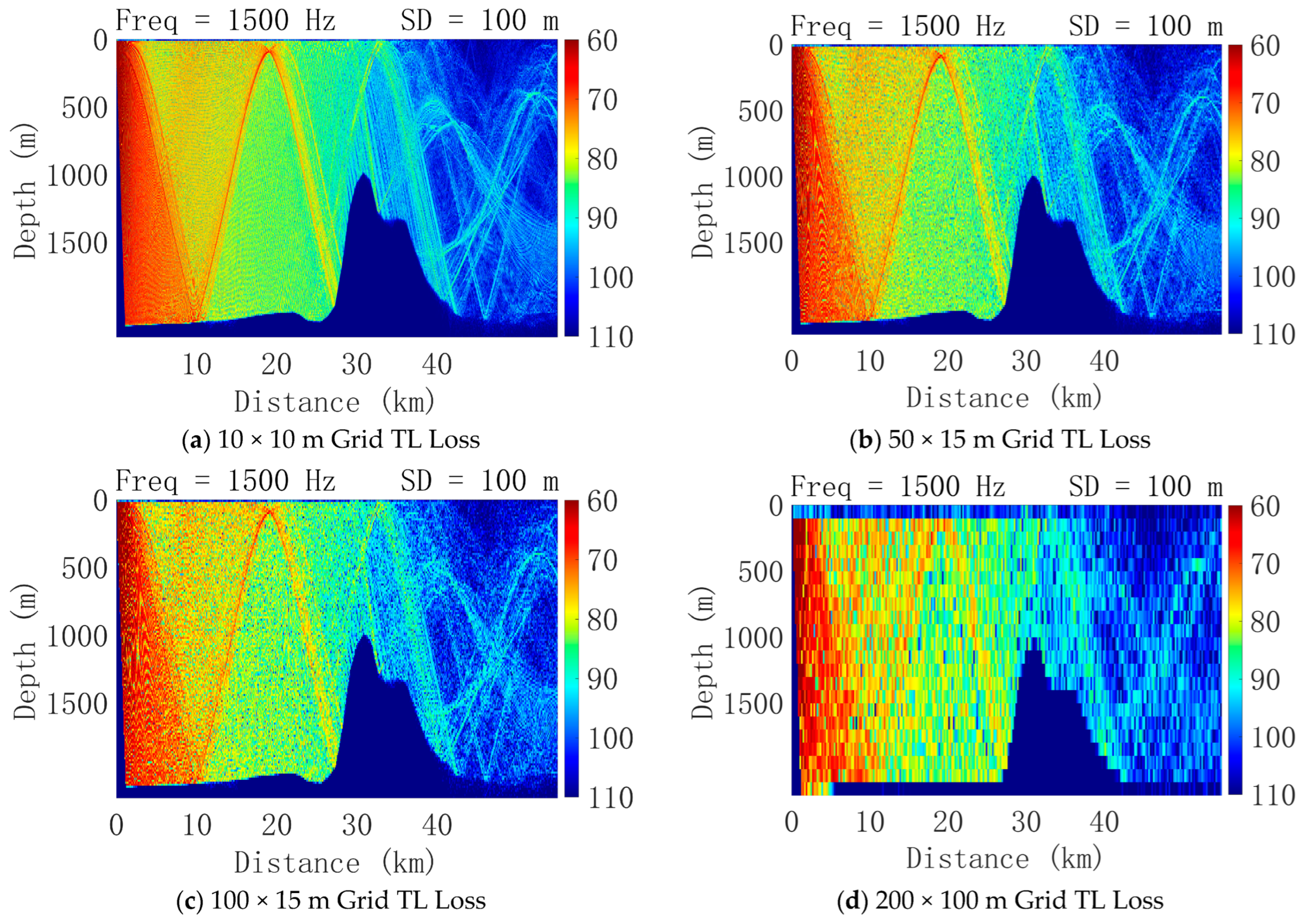
To evaluate the effectiveness of the adaptive-grid method under complex seabed topographic conditions, comparative simulations were conducted within a unified BELLHOP framework in terms of computational efficiency, numerical accuracy, and storage cost. Three typical seabed topographies, namely seamount, trench, and slope, were considered, and an adaptive-grid model was constructed for each case. The adaptive parameters used in this study were determined from representative test scenarios and should therefore be regarded as engineering-oriented empirical settings rather than uniformly optimal values for all ocean environments. For comparison, several uniform grids with different resolutions were also employed. To cover the range from high-resolution calculations to low-cost coarse simulations, four uniform-grid configurations were adopted: 10 × 10 m, 50 × 15 m, 100 × 15 m, and 200 × 100 m. The 10 × 10 m grid is used as the fine-grid benchmark in this study, mainly for qualitative validation of the acoustic-field distribution patterns. By contrast, the 50 × 15 m grid yields acoustic-field results that are highly consistent with those of the 10 × 10 m grid at a substantially lower computational cost, and is therefore adopted as a practical reference for RMSE evaluation.
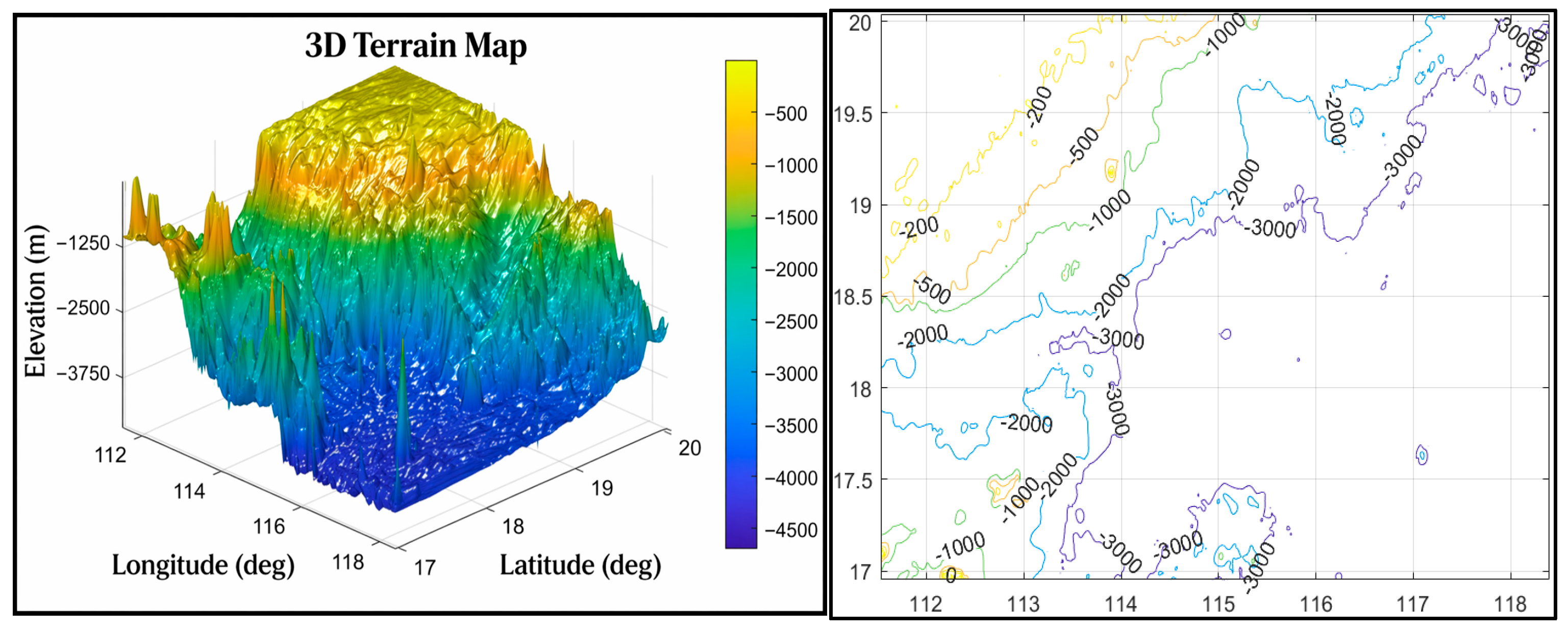
The study area is located in the transitional zone between the continental shelf and the deep-sea basin in the northern South China Sea, within 111.53° E–118.40° E and 16.95° N–20.04° N. The region includes a relatively complete set of topographic types, such as seamounts, trenches, and slopes, making it representative for deep-ocean acoustic propagation studies. As shown in Figure 3, the seabed topography generally deepens from northwest to southeast, exhibiting a typical transitional pattern. Owing to its rich and complex terrain, including regions with steep slopes and pronounced topographic variability, the area provides a suitable environmental setting for analyzing acoustic propagation characteristics under different topographic conditions and for validating the adaptive-grid construction method.
The numerical computations and program tests in this study were performed on a laptop computer equipped with a 13th Gen Intel(R) Core(TM) i9-13900HX processor with 24 CPU cores and 16 GB of RAM, running Windows 11. No GPU acceleration or other dedicated hardware acceleration techniques were used, and all experiments were conducted under the same hardware and software environment.
The simulations for the three topographic cases in this study were performed using the BELLHOP model, and the basic parameter settings are listed in Table 1. To ensure that the model can represent the acoustic propagation characteristics of a typical deep-ocean environment, the acoustic frequency was set to 1500 Hz, and the number of media layers was specified as NMEDIA = 1, indicating that a single-layer water-column environment was adopted in the calculation. The computational depth range was set to 0–2200 m to cover the entire water column and the seabed boundary. The source depth was fixed at 100 m for the seamount and slope cases and at 5 m for the trench case, so as to represent the deployment depth of the underwater acoustic source.
As shown in Table 2, to balance computational accuracy and efficiency, the propagation step size STEP was set to 200 m, which controls the numerical integration scale during ray tracing. The launch-angle range was specified as 60 ° to ensure effective coverage of the main propagation paths and multipath arrival structures. Since the focus of this study is on the influence of receiver-grid configuration rather than ray-tracing parameters, the BELLHOP STEP parameter and the launch-angle sampling settings were fixed for all comparative experiments, so that the observed differences could be attributed mainly to the receiver-grid design. These parameters together constitute the basic configuration of the BELLHOP simulations in this study. These parameter values are not claimed to be globally optimal for all ocean environments; they are tuned for the case-study region considered in this work and may require readjustment in other regions.

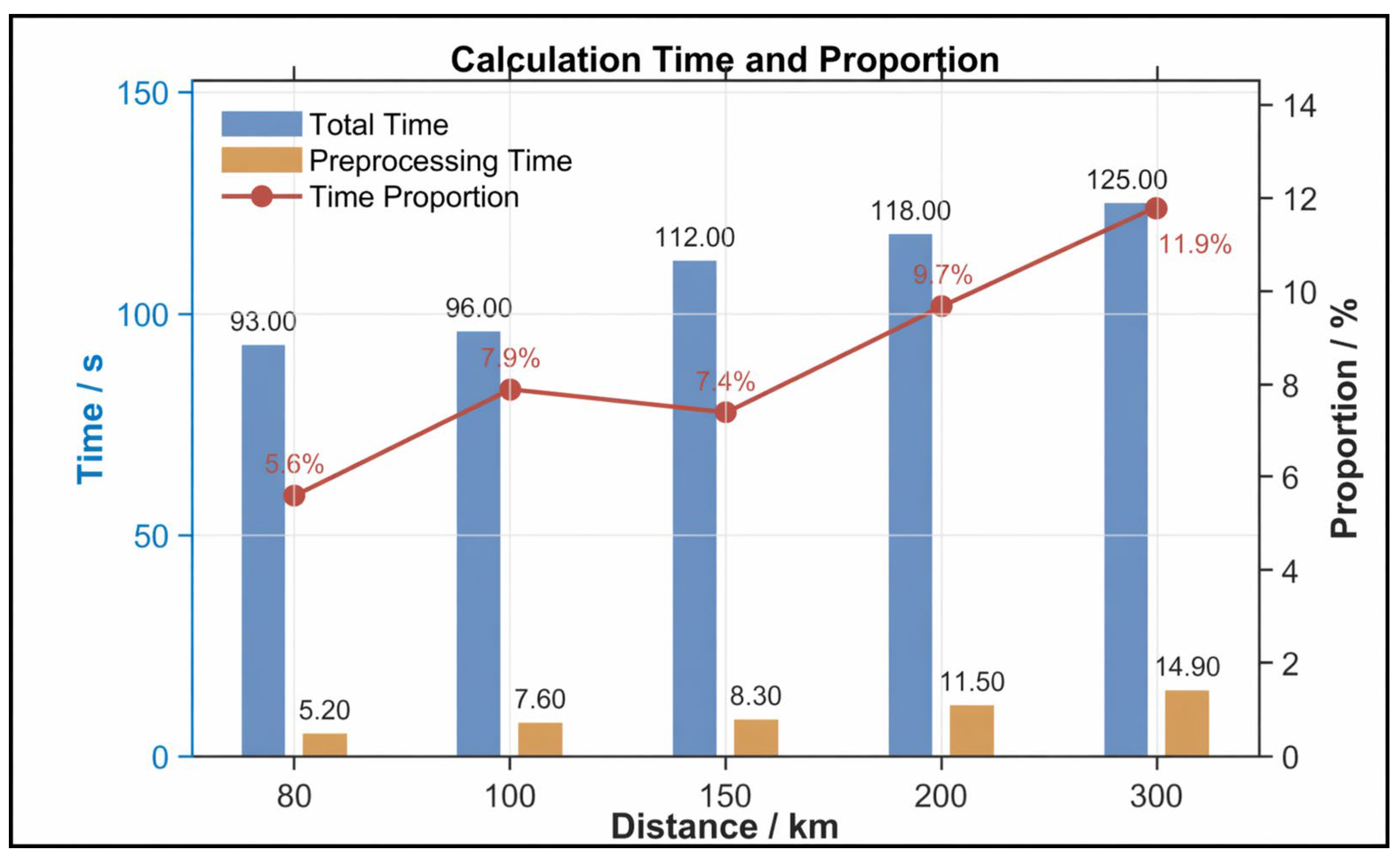
3.1. Analysis of Preprocessing Overhead in the Adaptive-Grid Model

To evaluate the influence of preprocessing on the overall computational cost of the adaptive-grid model, a dedicated statistical analysis of preprocessing time was performed under different propagation distances. The preprocessing procedure mainly includes grid generation, slope calculation, sound-speed-profile interpolation, and grid merging and refinement, and the results are shown in Figure 4. It can be seen that, although the preprocessing time increases with the horizontal propagation distance of the computational domain, its proportion in the total runtime remains low, ranging only from 5.6% to 11.9%. This indicates that the additional computational burden introduced by the preprocessing step is limited and does not significantly weaken the overall efficiency advantage of the adaptive-grid method. Overall, the preprocessing cost of the proposed method is controllable, and its main efficiency gain still comes from the subsequent acoustic-field solution stage, which further demonstrates its practical potential for large-scale acoustic propagation simulation.

3.2. Validation Based on Seamount Topography

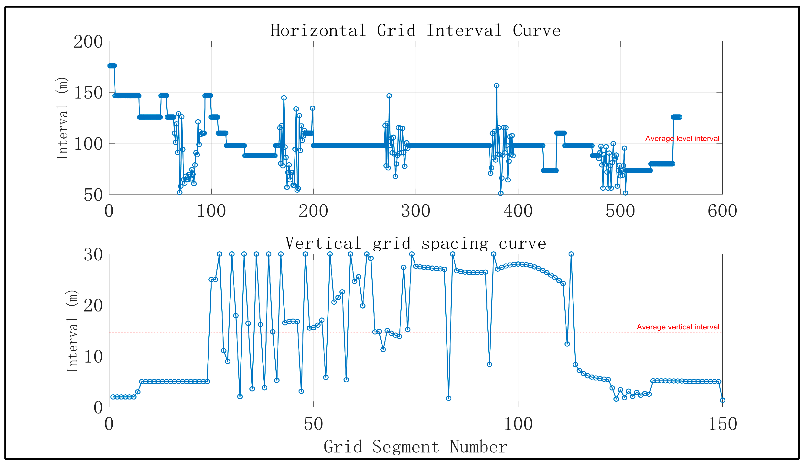
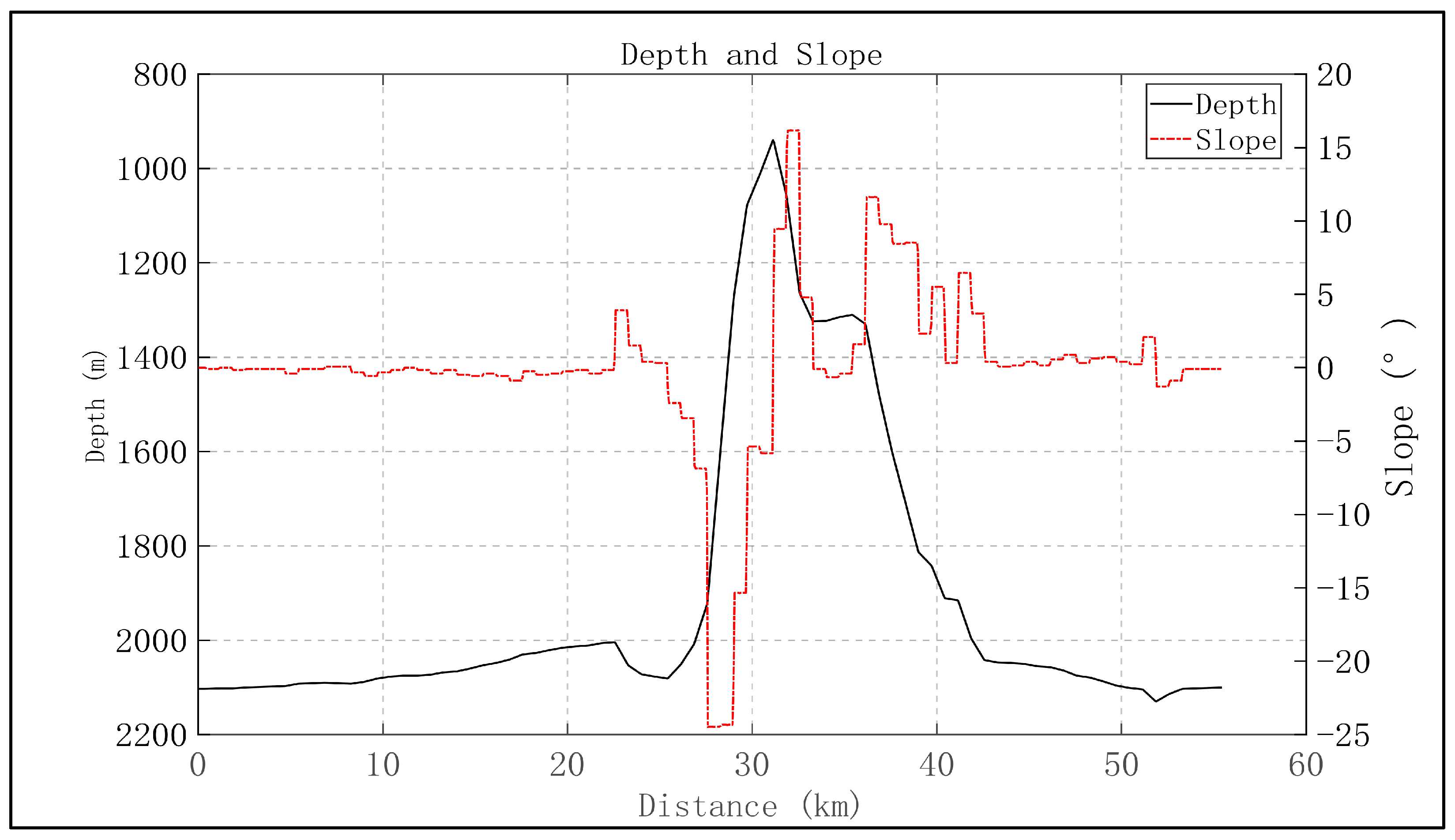
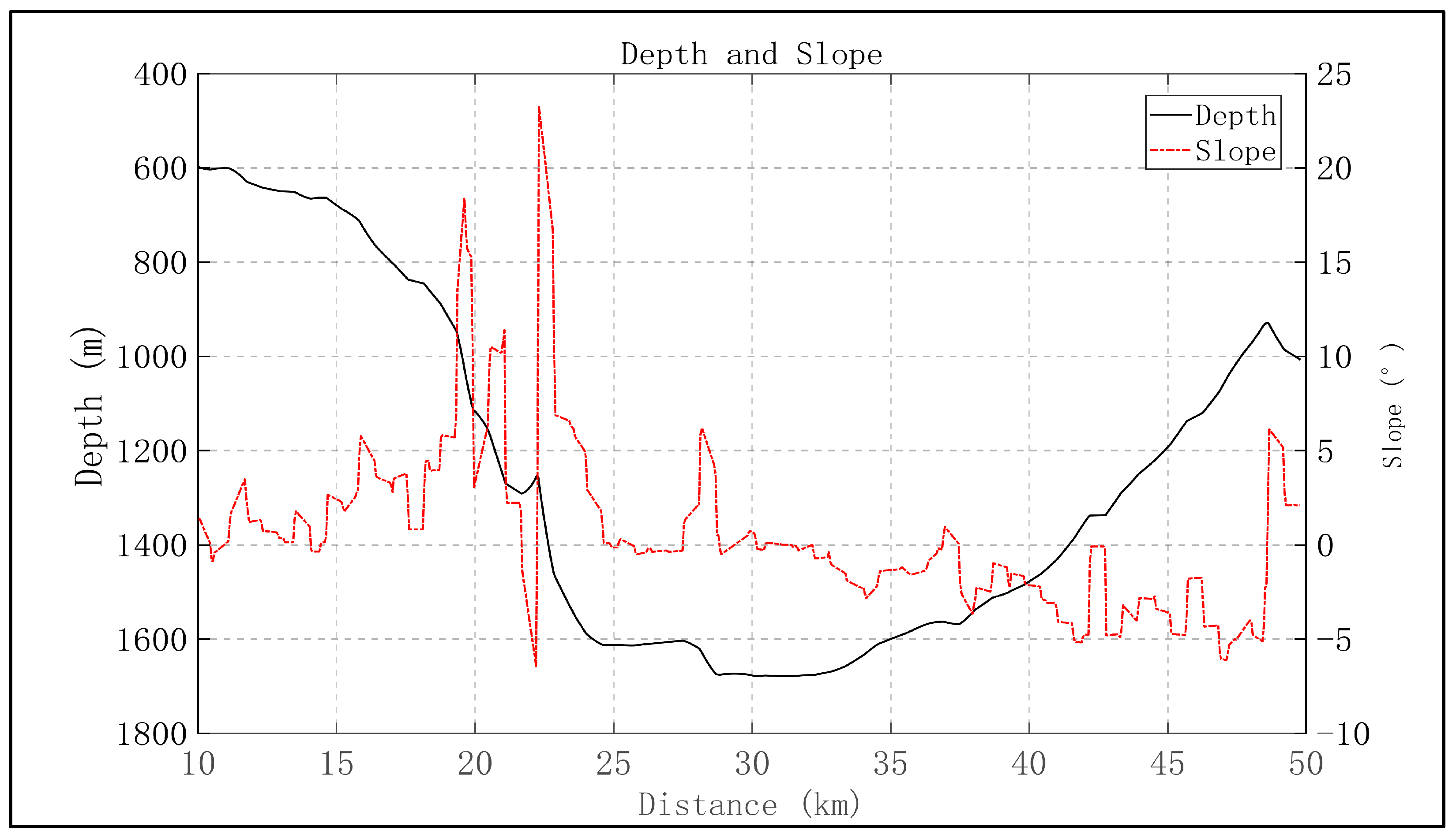
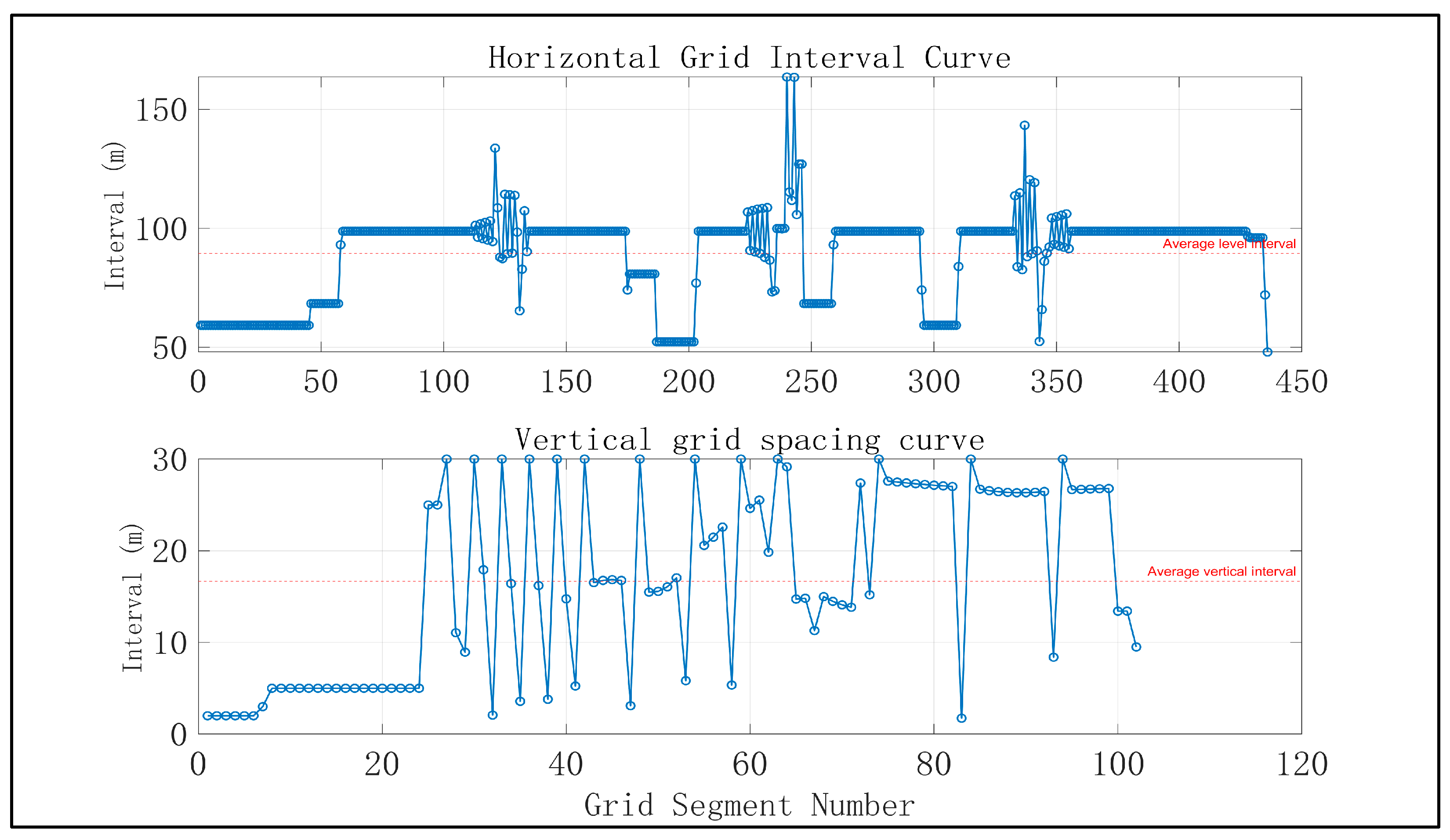
In the seamount experiment, a topographic slice was extracted from the terrain data shown in Figure 3. According to the slope distribution and sound-speed profile of the selected section, the receiver grid was adaptively adjusted, and the resulting horizontal and vertical grid spacings are shown in Figure 5 and Figure 6, respectively. The average horizontal and vertical spacings of the adaptive grid were 99.33 m and 14.67 m, which are close to those of the 100 × 15 m uniform grid, making it an appropriate reference for direct comparison of accuracy and computational cost. For comparative analysis, a 10 × 10 m grid was selected as the fine grid, a 50 × 15 m grid was adopted as the baseline grid to provide a relatively accurate reference solution, and a 100 × 15 m grid was used as a uniform grid with a resolution close to that of the adaptive grid, so that the performance of the proposed method could be evaluated more directly.
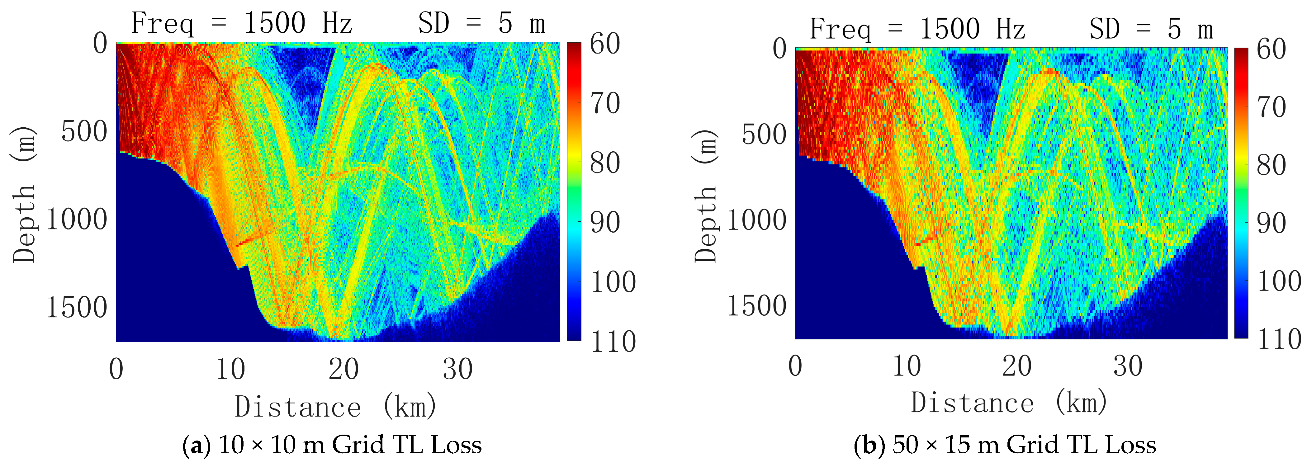
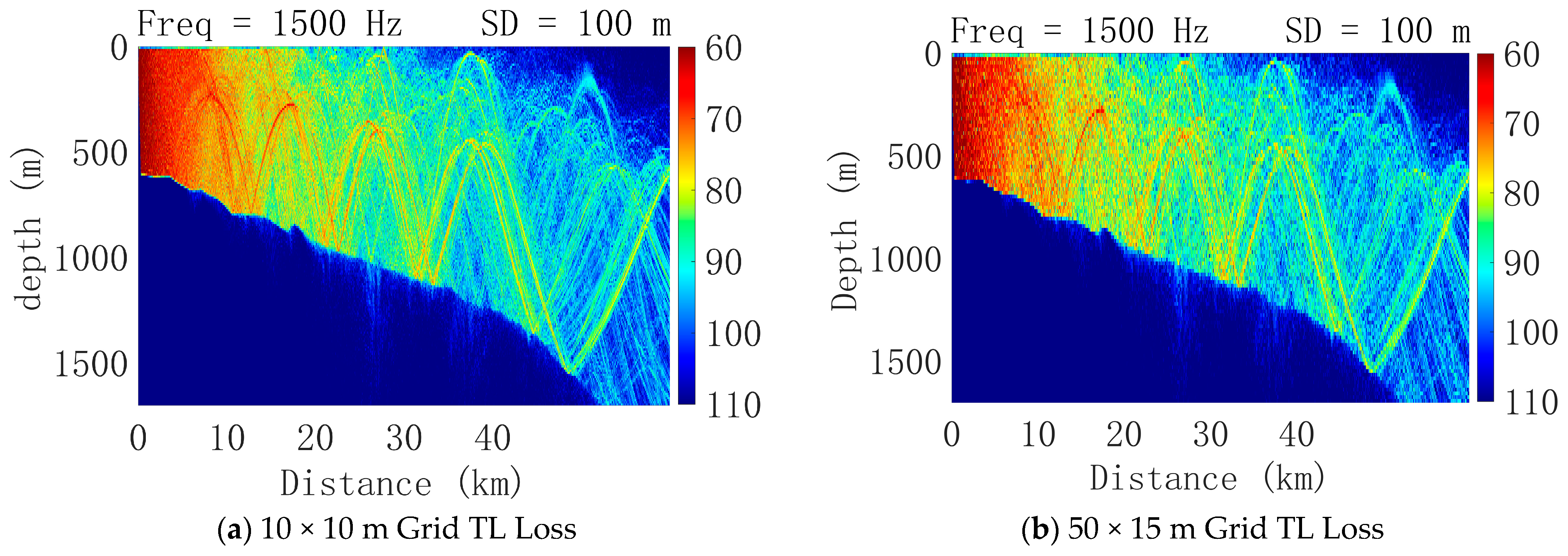
Under uniform-grid conditions, the BELLHOP acoustic-field results obtained at different resolutions exhibit clear differences in their ability to represent acoustic phenomena, such as interference fringes, energy-focusing regions, and terrain-induced shadow zones. As shown in Figure 7, the 10 × 10 m fine grid provides the most complete representation of the acoustic-field details associated with seamount topography, clearly resolving transmission-loss fluctuations, multipath interference structures, and local energy variations near the upslope, summit, and downslope regions. The 50 × 15 m baseline grid remains highly consistent with the fine-grid result in terms of the overall acoustic-field pattern, the major interference structures, and the main energy-distribution characteristics, and can therefore serve as a reliable reference solution for subsequent error evaluation. The 100 × 15 m uniform grid has an average resolution close to that of the adaptive grid and is still able to preserve the overall acoustic-field morphology and the dominant interference features, while offering lower computational cost than finer grids. In contrast, the 200 × 100 m coarse grid, owing to its excessively large horizontal and vertical sampling intervals, cannot adequately resolve the ray-bending effects and local acoustic-field distortions induced by topographic variations near the seamount. As a result, the interference fringes become excessively smoothed or even locally discontinuous, while typical acoustic features such as local focusing regions, near-bottom high-energy bands, and weak shadow zones behind the downslope are poorly represented.
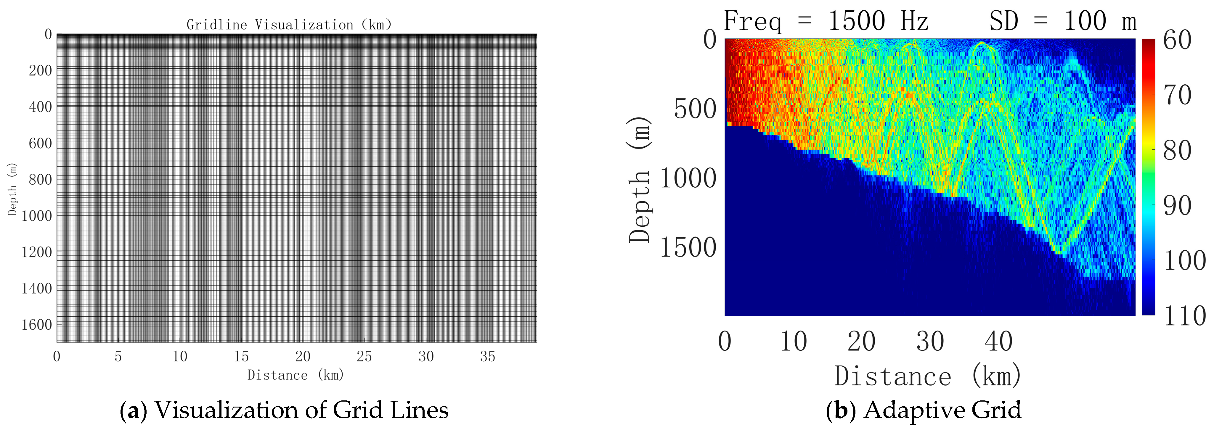
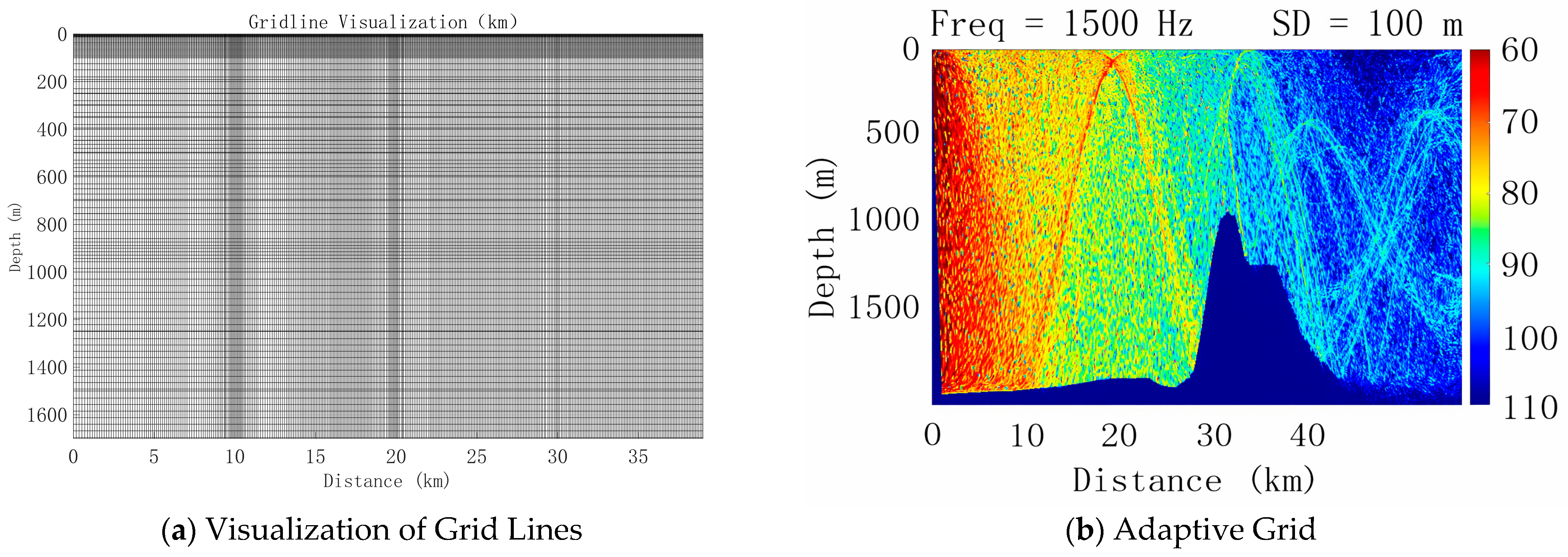
The adaptive-grid simulation was conducted using the horizontal and vertical grids derived from Figure 5 and Figure 6. The resulting grid-spacing distribution is shown in Figure 8a, and the corresponding two-dimensional transmission-loss field is presented in Figure 8b. Further analysis from the perspective of resolution indicates that the adaptive grid exhibits clear advantages in resolving local features under seamount topographic conditions. By refining the grid in regions with steep slopes and strong acoustic-field variations, the proposed method preserves the acoustic-field details more effectively in critical areas, such as the summit region, slope transition zones, and near-bottom sensitive regions, thereby enabling more accurate resolution of interference-fringe morphology, local energy extrema, and abrupt transmission-loss boundaries. Compared with uniform grids, the adaptive grid achieves higher effective resolution in key regions while keeping the overall number of grid nodes under control, thus improving the detail fidelity of acoustic-field simulations in complex seamount environments.
In addition to the 2D (two-dimensional) TL distributions, horizontal and vertical TL slices at selected depths and ranges were also examined. The adaptive-grid results were found to agree well with the reference-grid results in the phase and amplitude of the main interference fringes, which is also consistent with the corresponding RMSE values.
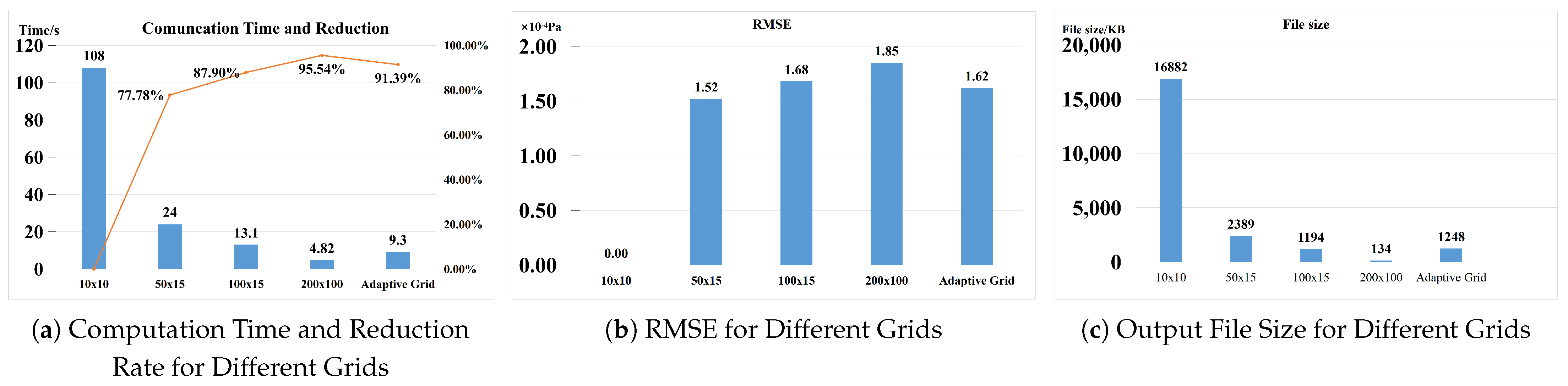
Figure 9a presents a comparison of the computational time among four uniform-grid configurations and the adaptive grid. As shown in the figure, the computational time of the uniform-grid model decreases markedly as the grid spacing increases, dropping from 108 s for the 10 × 10 m grid, which serves as the reference case, to 4.82 s for the 200 × 100 m grid. The computational time of the adaptive-grid model is 9.3 s, which is significantly lower than that of the 50 × 15 m grid and slightly lower than that of the 100 × 15 m grid. To quantitatively characterize the differences among transmission-loss fields obtained with different receiver-grid configurations, the root-mean-square error (RMSE) of transmission loss was calculated over the range–depth receiver grid in this study. Specifically, as shown in Equation (16), T L t e s t r i , z j and T L r e f r i , z j denote the transmission-loss values in dB at the receiver point r i , z j for the test grid and the reference grid, respectively, while N r and N z represent the numbers of receiver points in the range and depth directions, respectively. Therefore, the normalization in this study was performed by averaging over all receiver points on the entire range–depth grid. Figure 9b shows the comparison of RMSE values for the four grid configurations. A smaller RMSE indicates higher computational accuracy. It can be observed that the RMSE of the adaptive grid is close to that of the 100 × 15 m grid. This is mainly because, except for the seamount region, the other topographic features are relatively smooth and exhibit limited slope variation, causing the adaptive-grid result to be close to that of the corresponding uniform grid. Nevertheless, the adaptive grid achieves substantially higher accuracy than the 200 × 100 m grid, although its accuracy is slightly lower than that of the 50 × 15 m grid. In terms of file size, as shown in Figure 9c, the output file generated by the adaptive grid is markedly smaller than that of the 50 × 15 m grid.
R M S E T L = 1 N r N z i = 1 N r j = 1 N z T L t e s t r i , z j T L r e f r i , z j 2
It should be emphasized that this study does not seek to demonstrate rigorous convergence of the proposed method to the fine-grid solution. Instead, the comparative results show that the RMSE generally decreases as the effective average grid spacing is reduced. For the seamount case, the adaptive-grid result lies close to the overall RMSE trend formed by the uniform-grid results, indicating that its error behavior is consistent with the empirical pattern typically observed in conventional grid refinement.

3.3. Validation Based on Trench Topography

In the trench simulation experiment, a trench topographic slice was extracted from the terrain data shown in Figure 3. Based on the slope distribution and sound-speed profile of the selected section, the receiver grid was adaptively adjusted, and the resulting horizontal and vertical grid spacings are presented in Figure 10 and Figure 11, respectively. The adaptive grid yielded average horizontal and vertical spacings of 89.52 m and 16.45 m, respectively. The grid sizes selected for comparison were consistent with those used in the seamount case in Section 3.1.
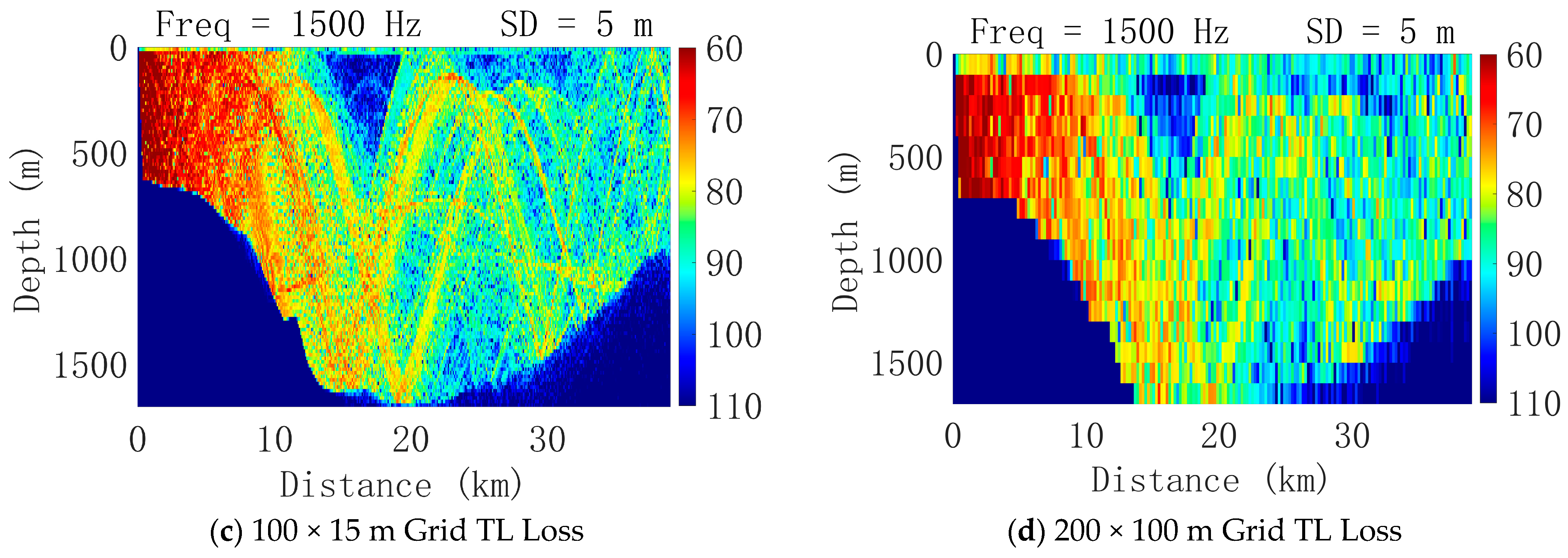
Under uniform-grid conditions, the BELLHOP results for the trench case also show clear resolution-dependent differences in acoustic-field representation. As shown in the corresponding Figure 12, the 10 × 10 m fine grid provides the most complete resolution of the trench acoustic field, clearly capturing transmission-loss fluctuations, interference structures, and local energy variations associated with the trench sidewalls and bottom region. The 50 × 15 m baseline grid remains highly consistent with the fine-grid result in terms of the overall field pattern and the dominant interference features, and is therefore adopted as the reference solution. The 100 × 15 m uniform grid, whose resolution is close to that of the adaptive grid, still preserves the main acoustic-field morphology and the principal interference characteristics while reducing computational cost. In contrast, the 200 × 100 m coarse grid cannot adequately resolve the complex acoustic-field variations induced by the trench topography, leading to excessive smoothing of interference structures and weakened representation of local energy-concentration regions and trench-bottom acoustic features.
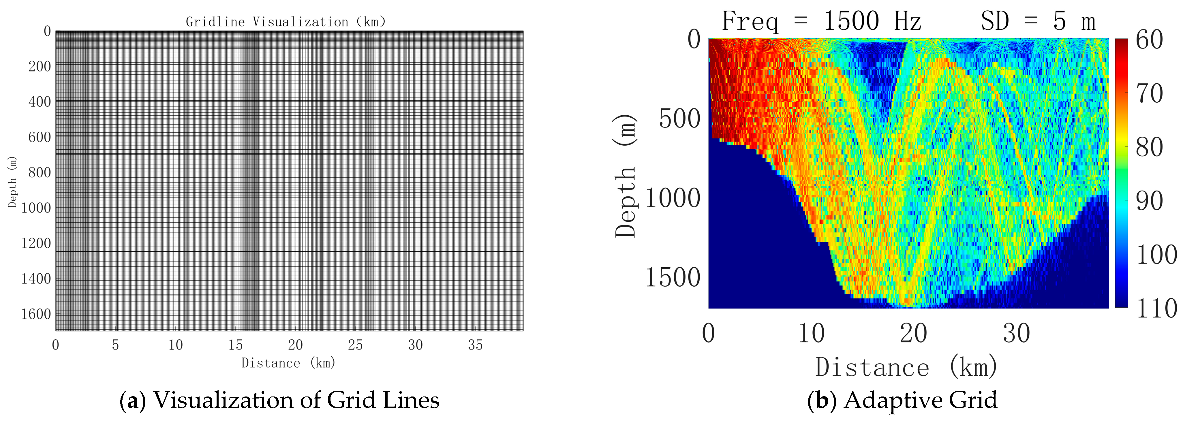
The adaptive-grid simulation for the trench case was performed using the horizontal and vertical grids derived from Figure 10 and Figure 11. The resulting grid-spacing distribution is shown in Figure 13a, and the corresponding two-dimensional transmission-loss field is presented in Figure 13b. From the perspective of resolution, the adaptive grid shows clear advantages in resolving local acoustic-field features under trench topography. By refining the grid in regions with steep sidewalls and strong field variation, the method more effectively preserves the details of sidewall-reflection zones, trench-bottom energy concentration, and local multipath structures.
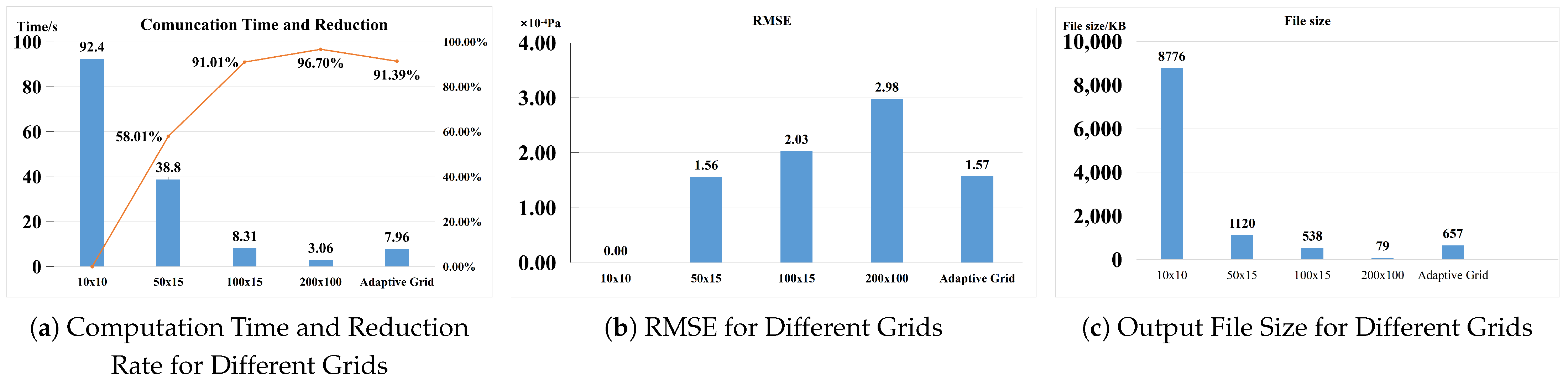
Figure 14 presents a comparison of computational time, RMSE, and output file size for simulations under trench topography using the adaptive grid and uniform grids with different resolutions. The computational time of the adaptive grid is 7.96 s, which is comparable to that of the 100 × 15 m grid and significantly shorter than that of the 50 × 15 m grid. In terms of computational accuracy, the adaptive grid shows only a small difference from the 50 × 15 m grid, while remaining clearly more accurate than the 100 × 15 m and 200 × 100 m grids. With respect to file size, the adaptive-grid output is 657 KB, which is substantially smaller than the 1120 KB obtained with the 50 × 15 m grid.

3.4. Validation Based on Slope Terrain

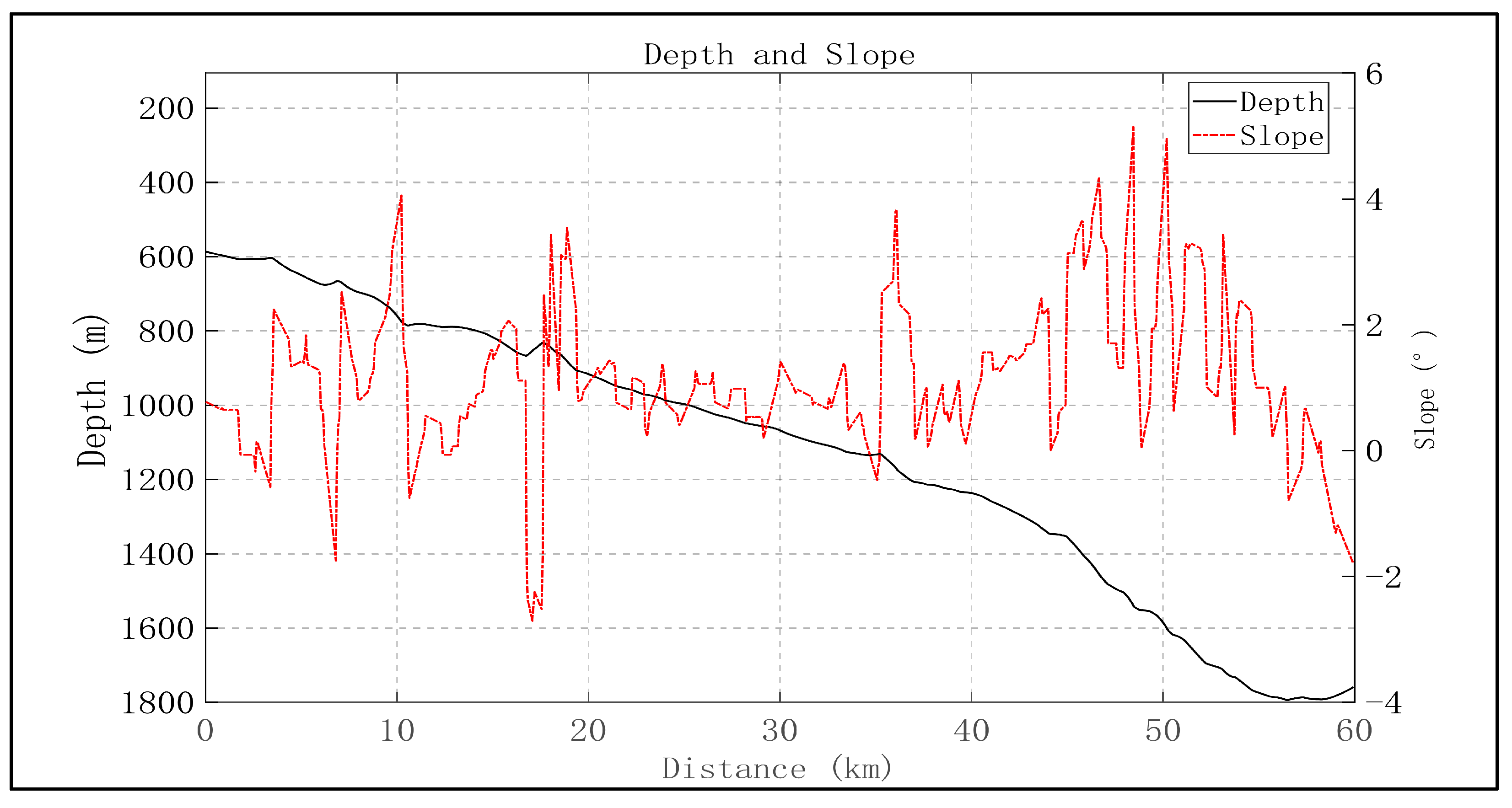
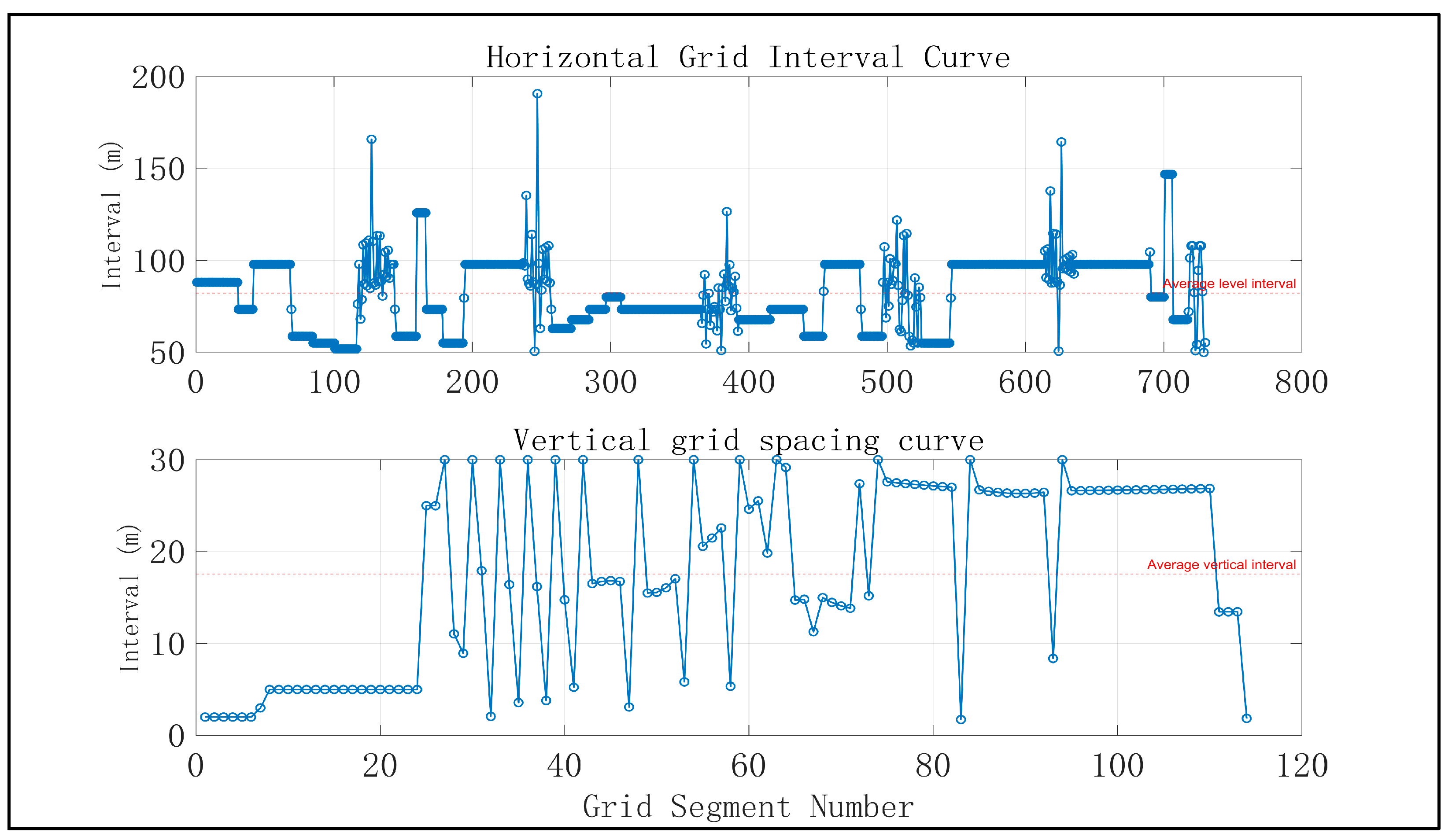
In the slope simulation experiment, a slope topographic slice was extracted from the terrain data shown in Figure 3. Based on the slope distribution and sound-speed profile of the selected section, the receiver grid was adaptively adjusted, and the resulting horizontal and vertical grid spacings are shown in Figure 15 and Figure 16. The adaptive grid yielded average horizontal and vertical spacings of 81.55 m and 17.54 m, respectively. The grid configurations selected for comparison were consistent with those adopted in the seamount and trench cases above.
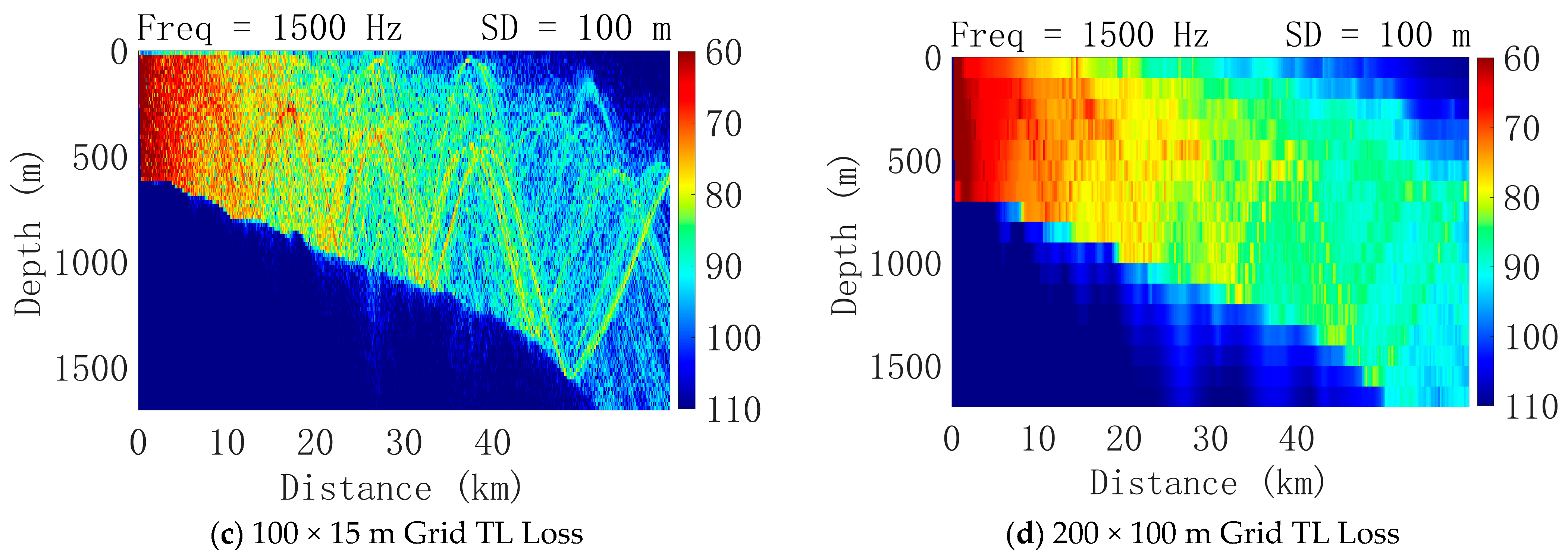
As shown in the corresponding Figure 17, under uniform-grid conditions, the 10 × 10 m fine grid provides the most complete representation of the slope acoustic field, clearly capturing transmission-loss fluctuations, interference structures, and local energy variations associated with the sloping bottom and near-bottom region. The 50 × 15 m baseline grid remains highly consistent with the fine-grid result in terms of the overall field pattern and the dominant interference features, and is therefore adopted as the reference solution. The 100 × 15 m uniform grid, whose resolution is close to that of the adaptive grid, still preserves the main acoustic-field morphology and the principal interference characteristics while reducing computational cost. In contrast, the 200 × 100 m coarse grid cannot adequately resolve the continuous acoustic-field variations induced by the slope topography, leading to excessive smoothing of interference structures and weakened representation of near-bottom energy variations and slope-induced field transitions.
The adaptive-grid simulation for the slope case was performed using the horizontal and vertical grids derived from Figure 15 and Figure 16. The resulting grid-spacing distribution is shown in Figure 18a, and the corresponding two-dimensional transmission-loss field is presented in Figure 18b. From the perspective of resolution, the adaptive grid also shows clear advantages in resolving local acoustic-field features under slope topography. By refining the grid in regions with larger bottom gradients and stronger acoustic-field variation, the method more effectively preserves the details of near-bottom energy variation, interference-structure evolution, and slope-induced acoustic-field transitions.
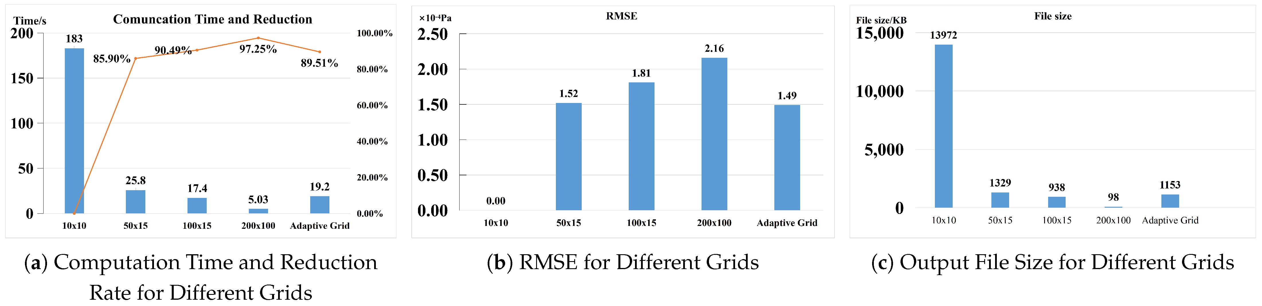
Figure 19 presents a comparison of computational time, RMSE, and output file size between the adaptive grid and uniform grids with different resolutions under slope topography. The results show that the computational time of the adaptive grid is 19.2 s, which is close to that of the 100 × 15 m uniform grid and significantly lower than that of the 50 × 15 m grid, indicating that the adaptive grid maintains relatively high resolution while achieving good computational efficiency. In terms of computational accuracy, the RMSE of the adaptive grid was 1.49 dB, compared with 1.52 dB for the 50 × 15 m grid, corresponding to a relative reduction of 1.97%. Although the improvement is modest, it still indicates a slight accuracy advantage for the adaptive grid in this scenario. But its RMSE is clearly lower than that of the 100 × 15 m and 200 × 100 m uniform grids, demonstrating that it can more effectively balance accuracy and efficiency in the slope environment. Regarding output file size, the adaptive-grid result is 1153 KB, which is substantially smaller than the 1329 KB produced by the 50 × 15 m grid, although slightly larger than the 938 KB obtained with the 100 × 15 m grid. Overall, the adaptive grid exhibits favorable comprehensive performance under slope topographic conditions.

4. Conclusions

4.1. Summary

This study proposed an adaptive receiver-grid method for the BELLHOP model, in which the horizontal and vertical grid spacings were dynamically adjusted according to bathymetric slope and sound-speed-profile gradient, respectively, under spacing and layer constraints. The method was validated in three representative environments, namely seamount, trench, and slope cases. The results showed that, in the tested environments, the RMSE of the adaptive grid was comparable to or lower than that of the medium-resolution grid (100 × 15 m), and in the slope case, it was slightly lower than that of the 50 × 15 m grid. Meanwhile, compared with the fine-resolution uniform grid, the adaptive grid reduced computational time and storage cost by approximately 85–90%, with this advantage becoming more evident in environments with stronger topographic variation. In addition, compared with the uniform grid having the closest error level, the adaptive grid further reduced computational time and output file size while maintaining comparable accuracy.
Overall, the proposed method achieved a better balance between computational efficiency and numerical accuracy. It significantly reduced the computational and storage costs without noticeably degrading the sound-field solution quality. These results indicate that the proposed method is well-suited for efficient acoustic propagation simulation in complex ocean environments and has strong potential for practical engineering applications.

4.2. Expectation

The present study focuses on the adaptive optimization of receiver-grid parameters and their practical effectiveness, rather than on a formally analyzed adaptive scheme with a rigorous convergence proof. Therefore, no strict theoretical convergence toward the fine-grid reference solution is claimed. The numerical results only indicate an empirical trend whereby the error decreases as the grid is refined and the adaptive-grid results approach the fine-grid reference in the tested cases. Since the method mainly adjusts the receiver grid, its influence is primarily on acoustic-field sampling and spatial representation, with limited direct impact on the ray-integration procedure of BELLHOP. No obvious numerical instability caused by local refinement was observed in the seamount, trench, or slope cases. The current refinement strategy is guided by a priori environmental indicators, namely bathymetric slope and sound-speed-profile gradient, rather than by a posteriori error estimators, ray density, or wavelength-based criteria. These more rigorous adaptive strategies will be considered in future work.
It should be noted that the present performance evaluation was conducted for a single representative frequency (1500 Hz) and within the specific study region considered in this work. Extension of the proposed method to other frequencies and broader ocean environments will be investigated in future studies.
The present study treats horizontal and vertical grid adaptation independently, using bathymetric slope and SSP gradient as separate control variables. This is an engineering-oriented simplification that reduces implementation complexity while capturing the dominant effects of bathymetric and SSP variations on receiver-grid distribution. For the tested cases, this strategy provides a reasonable balance between efficiency and accuracy. However, in regions with strong bathymetry–SSP interaction, its ability to represent fully coupled two-dimensional propagation behavior may remain limited. Fully coupled two-dimensional adaptive criteria based on acoustic-field variability or ray density will be investigated in future work.
In future work, the proposed adaptive receiver-grid strategy may be further integrated with GPU-based parallel computing. The adaptive grid can reduce the computational scale by decreasing redundant receiver points, while GPU acceleration can further improve the efficiency of the remaining acoustic-field calculations. Such a combination may provide a more effective pathway for large-scale and real-time acoustic propagation modeling. A dedicated implementation and performance evaluation of this coupled framework will be investigated in future studies.

Author Contributions

Conceptualization, Z.L. (Zhichao Lv), Z.L. (Zongwei Liu), F.Y. and K.Z.; methodology, K.Z.; software, K.Z.; validation, Z.L. (Zongwei Liu), Z.L. (Zhichao Lv) and K.Z.; formal analysis, J.C. (Junjie Chen), J.C. (Jialong Chen) and C.T.; investigation, Z.L. (Zongwei Liu); resources, Z.L. (Zongwei Liu); data curation, K.Z., F.Y.; writing—original draft preparation, Z.L. (Zhichao Lv) and K.Z. writing—review and editing, Z.L. (Zongwei Liu), Z.L. (Zhichao Lv) and K.Z.; visualization, Z.L. (Zhichao Lv), Z.L. (Zongwei Liu), C.T., J.C. (Jialong Chen) and C.T.; supervision, Z.L. (Zhichao Lv), Z.L. (Zongwei Liu), F.Y. and K.Z.; project administration, Z.L. (Zongwei Liu), Z.L. (Zhichao Lv), J.C. (Junjie Chen) and C.T.; funding acquisition, Z.L. (Zongwei Liu), F.Y., Z.L. (Zhichao Lv), J.C. (Jialong Chen) and J.C. (Junjie Chen) All authors have read and agreed to the published version of the manuscript.

Funding

This research was funded by the National Key Research and Development Program of China, grant number 2023YFE0201900; the Key Research and Development Program of Shandong Province, grant number 2025CXPTWZ004; the Underwater Unmanned Platform Acoustic Signal Perception and Early Warning Technology Research Project, grant number SKLA202504; National Natural Science Foundation of China, grant number 42506258; Key Laboratory of Marine Environmental Survey Technology and Application, Ministry of Natural Resources, P. R. China, grant number MESTA-2023-B005.

Data Availability Statement

The data presented in this study are available upon request from the corresponding author due to laboratory confidentiality regulations.

Conflicts of Interest

The authors declare that the research was conducted in the absence of any commercial or financial relationships that could be construed as potential conflicts of interest.

References

  1. Yang, S.E. Principles of Underwater Acoustic Propagation; Harbin Engineering University Press: Harbin, China, 1994; Volume 1. [Google Scholar]
  2. Liu, B.S.; Huang, Y.W.; Chen, W.J.; Lei, J.Y. Principles of Underwater Acoustics, 3rd ed.; Science Press: Beijing, China, 2019. [Google Scholar]
  3. Thuillier, O.; Le Josse, N.; Olteanu, A.L.; Sevaux, M.; Tanguy, H. Heterogeneous multistatic sonar networks optimization: Literature review and preliminary enhancements. Eur. J. Oper. Res. 2026, 329, 405–425. [Google Scholar] [CrossRef]
  4. Pal, A.; Campagnaro, F.; Ashraf, K.; Rahman, M.R.; Ashok, A.; Guo, H. Communication for underwater sensor networks: A comprehensive summary. ACM Trans. Sens. Netw. 2023, 19, 1–44. [Google Scholar] [CrossRef]
  5. Gao, T.Q.; Chen, H.Y.; Zhang, J.M.; Li, K. Research on underwater multi-target tracking algorithm based on the BELLHOP model. Tech. Acoust. 2023, 42, 248–255. [Google Scholar]
  6. Zhang, G.; Zhang, L.; Wang, Y.; Ma, Y.; Zhou, X.; Yu, Y. Spatiotemporal analysis of sonar detection range in Luzon Strait. J. Mar. Sci. Eng. 2024, 12, 1191. [Google Scholar] [CrossRef]
  7. Umamaheswararao, S.; Kumar, M.N.V.S.S.; Madhu, R. Wireless underwater channel modelling for acoustic communication. Int. J. Comput. Vis. Robot. 2024, 14, 529–539. [Google Scholar] [CrossRef]
  8. Huang, J.Q.; Ju, J.B. Simulation study on shallow-water acoustic propagation based on a ray model. Mod. Electron. Tech. 2011, 34, 94–96. [Google Scholar]
  9. Yang, J.X.; Shuai, C.G.; He, L. Progress in the application of ray theory to shallow-water acoustic propagation. In Proceedings of the 15th Symposium on Ship Underwater Noise, Chennai, India, 23–25 February 2015; pp. 616–622. [Google Scholar]
  10. Li, M.H.; Chen, C.; Feng, X.; Wang, C.; Wang, H. Frequency adaptability analysis of typical acoustic propagation models. Front. Mar. Sci. 2025, 12, 1687199. [Google Scholar] [CrossRef]
  11. Porter, M.B. The BELLHOP Manual and User’s Guide: Preliminary Draft; Technical Report; Heat, Light, and Sound Research, Inc.: San Diego, CA, USA, 2011; p. 260. [Google Scholar]
  12. Xu, C.X. Research on Three-Dimensional Acoustic Field Modeling and Fast Computation Based on Parabolic Equation Approximation. Ph.D. Thesis, Harbin Engineering University, Harbin, China, 2017. [Google Scholar]
  13. Ren, C.; Huang, Y.-W.; Xia, Z. Modeling of spatial correlation characteristics of broadband ocean ambient noise vector field. Acta Phys. Sin. 2022, 71, 024301. [Google Scholar] [CrossRef]
  14. Wilkes, D.R.; Gourlay, T.P.; Gavrilov, A.N. Numerical modeling of radiated sound for impact pile driving in offshore environments. IEEE J. Ocean. Eng. 2016, 41, 1072–1078. [Google Scholar] [CrossRef]
  15. Chen, L.R.; Peng, Z.H. Parallel Algorithm Design of the Gaussian Ray Acoustic Field Model in an MPI Environment; Chinese Society of Acoustics, Underwater Acoustics Committee: Beijing, China, 2011; pp. 40–42. [Google Scholar]
  16. Zhang, Z.J.; Sun, B.W. Parallelization of the Bellhop ray model. Appl. Acoust. 2019, 38, 1–7. [Google Scholar] [CrossRef]
  17. Stålberg, J.; Ulmstedt, M. GPU accelerated ray-tracing for simulating sound propagation in water. Digit. Vetenskapliga Ark. 2019, 89. [Google Scholar]
  18. Chen, Y.E.; An, L. Parallel design of the Bellhop model based on CUDA. In Proceedings of the 5th Underwater Unmanned Systems Technology Forum, Guangzhou, China, 28–30 October 2022; Southeast University Key Laboratory of Underwater Acoustic Signal Processing, Ministry of Education: Nanjing, China, 2022; pp. 69–74. [Google Scholar]
  19. Liu, W.; Hu, S.; Li, H. Modeling and fast computation of submarine stealth effectiveness. Ship Sci. Technol. 2023, 45, 39–46. [Google Scholar]
  20. Roberts, K.J.; Pringle, W.J.; Westerink, J.J. OceanMesh2D 1.0: MATLAB-based software for two-dimensional unstructured mesh generation in coastal ocean modeling. Geosci. Model Dev. 2019, 12, 1847–1868. [Google Scholar] [CrossRef]
  21. Jensen, F.B.; Kuperman, W.A.; Porter, M.B. Computational Ocean Acoustics; Springer: New York, NY, USA, 2011. [Google Scholar]
  22. Monteiro, N.M.R.; Oliveira, T.C.A. Mesh generation for underwater acoustic modeling with KRAKEN. Adv. Eng. Softw. 2023, 180, 103455. [Google Scholar] [CrossRef]
  23. Chen, C.T.; Millero, F.J. Speed of sound in seawater at high pressures. J. Acoust. Soc. Am. 1977, 62, 1129–1135. [Google Scholar] [CrossRef]
  24. Yan, J.J. Design and Implementation of Rapid Sonar Range Prediction Software for Small-Memory Systems. Master’s Thesis, Harbin Engineering University, Harbin, China, 2023. [Google Scholar]
  25. Lan, Q.; Ma, S.Q.; Piao, S.C.; Xiao, W.; Wang, Y. Multi-core parallelization and performance evaluation of the BELLHOP3D model. Tech. Acoust. 2024, 43, 468–473. [Google Scholar]
  26. Ke, L.; Wu, S. Acoustic propagation characteristics of horizontally varying double duct waveguides under Arctic ice. J. Mar. Sci. 2024, 42, 47–57. [Google Scholar] [CrossRef]
  27. Tang, J.; Cui, P.C.; Zhang, J.; Zhou, N.C.; Wu, X.J.; Gong, X.Q.; Zhang, Y.B. Review of mesh adaptation for fluid numerical simulation. Adv. Mech. 2023, 53, 661–692. [Google Scholar]
  28. Jiang, C.; Xu, C.; He, Y.; Feng, W.; Chai, J. Underwater acoustic propagation models with transformers. In Proceedings of the 2024 3rd International Conference on Cloud Computing, Big Data Application and Software Engineering (CBASE), Hangzhou, China, 11–13 October 2024; pp. 727–731.
  29. Sun, Z.; Wang, Y.; Liu, W. End-to-end underwater acoustic transmission loss prediction with adaptive multi-scale dilated network. J. Acoust. Soc. Am. 2025, 157, 382–395. [Google Scholar] [CrossRef]
  30. Yin, L.J.; Zhang, L.; Sun, X.H.; Duan, J.; Da, L. Influence of topography and the Kuroshio on sound propagation in the Okinawa Sea area in winter. Acta Acust. 2023, 48, 802–810. [Google Scholar]
  31. Hersbach, H.; Comyn-Platt, E.; Bell, B.; Berrisford, P.; Biavati, G.; Horányi, A.; Muñoz Sabater, J.; Nicolas, J.; Peubey, C.; Radu, R.; et al. ERA5 Post-Processed Daily Statistics on Pressure Levels from 1940 to Present. Copernicus Climate Change Service (C3S) Climate Data Store (CDS) [Dataset] 2024. Available online: https://cds.climate.copernicus.eu/datasets/derived-era5-pressure-levels-daily-statistics?tab=overview (accessed on 16 April 2026). [CrossRef]
  32. Chen, J.; Li, Z.; Lv, Z.; Wang, L.; Li, H.; Shi, Y. Analysis of acoustic propagation characteristics in the Okinawa Sea region beneath fluctuating sea surfaces. In Proceedings of the 2024 7th International Conference on Information Communication and Signal Processing (ICICSP), Zhoushan, China, 21–23 September 2024; IEEE: New York, NY, USA, 2024; pp. 735–739. [Google Scholar]
  33. Zhu, Y.Q. Influence of Typical Deep-Sea Seabed Topography on Acoustic Propagation Characteristics. Audio Eng. 2021, 45, 9–11+16. [Google Scholar] [CrossRef]
  34. Han, J.; Huang, J.G.; Cao, H.W. Ocean channel simulation software HJRAY and its application in underwater acoustic communication. J. Syst. Simul. 2007, 19, 35–37. [Google Scholar]
  35. Brekhovskikh, L.M.; Lysanov, Y.P. Fundamentals of Ocean Acoustics, 3rd ed.; Springer: New York, NY, USA, 2003. [Google Scholar]
  36. Mitra, A.; Panda, J.P.; Warrior, H.V. Experimental and numerical investigation of the hydrodynamic characteristics of Autonomous Underwater Vehicles over sea-beds with complex topography. Ocean. Eng. 2020, 198, 106978. [Google Scholar] [CrossRef]
  37. Sun, X.; Zhang, S.; Chen, F.; Wang, P. Coupling Effect of the Bottom Type-Depth Configuration on the Sonar Detection Range in Seamount Environments. J. Mar. Sci. Eng. 2026, 14, 89. [Google Scholar] [CrossRef]
  38. McKinley, M.; Liu, G.; Touret, R.X.; O’Donnell, B.; Bracco, A.; Sabra, K.G. Impact of vertical resolution in a regional ocean circulation model of the northern Gulf of Mexico for acoustic predictions in the upper ocean. J. Acoust. Soc. Am. 2025, 157, 2191–2205. [Google Scholar] [CrossRef]
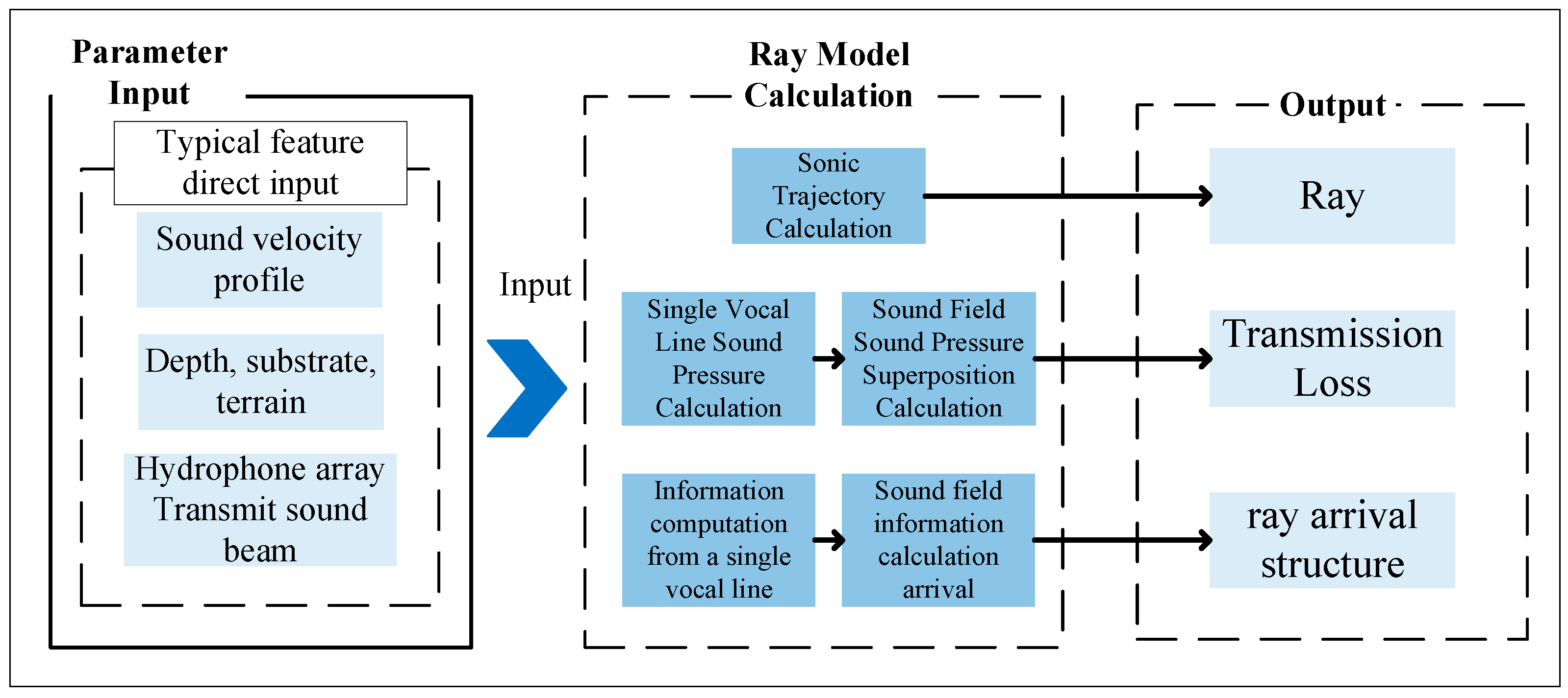
Figure 2. Flowchart of the BELLHOP model.
Jmse 14 00756 g002
Figure 3. Three-dimensional terrain and contour maps.
Jmse 14 00756 g003
Figure 4. Calculation time and proportion of adaptive-grid model.
Jmse 14 00756 g004
Figure 5. Seamount topographic slope map.
Jmse 14 00756 g005
Figure 6. Seamount grid-spacing profile.
Jmse 14 00756 g006
Figure 7. Comparison of 2D seamount transmission loss resolution under different grids.
Jmse 14 00756 g007
Figure 8. Seamount grid-line visualization and acoustic field of the adaptive grid.
Jmse 14 00756 g008
Figure 9. Simulation results with different grids in seamount topography.
Jmse 14 00756 g009
Figure 10. Trench topographic slope map.
Jmse 14 00756 g010
Figure 11. Trench grid-spacing profile.
Jmse 14 00756 g011
Figure 12. Comparison of 2D trench transmission loss resolution under different grids.
Jmse 14 00756 g012aJmse 14 00756 g012b
Figure 13. Trench grid-line visualization and acoustic field of the adaptive grid.
Jmse 14 00756 g013
Figure 14. Simulation results with different grids in trench topography.
Jmse 14 00756 g014
Figure 15. Slope terrain and slope map.
Jmse 14 00756 g015
Figure 16. Slope grid-spacing profile.
Jmse 14 00756 g016
Figure 17. Comparison of 2D slope transmission loss resolution under different grids.
Jmse 14 00756 g017aJmse 14 00756 g017b
Figure 18. Slope grid-line visualization and acoustic field of the adaptive grid.
Jmse 14 00756 g018
Figure 19. Simulation results with different grids in slope topography.
Jmse 14 00756 g019
Table 1. Results of the sensitivity coefficient analysis.
Sensitivity Coefficient α Runtime (s)RMSE (Pa)Explanation
103.22.64Insufficient encryption
203.32.59
403.72.29
604.12.13
1004.41.51Better balance
1204.91.49Limited improvement
1505.61.48
1707.21.50Over-encryption
Table 2. Basic simulation parameters of the BELLHOP model.
InputExplanation
TittleBasic Settings
Frequency [Hz]1500
NMEDIA1
Option1‘CVWT’Sea surface setup
Nmesh  Roughness  z(nssp)51  0.0  2200
Depth(1)  cp(1)0.0000  1545.1457/Sound Velocity Profile Settings
…   ……   …
…   ……   …
Depth(nssp) cp(nssp)2200.0000  1579.1258
Option2‘A~’Seabed Parameters
Settings
Bottom2200  1700.00 0.0 1.8 0.8/
NSD1Output Parameter Settings
SD(1:NSD)100/
NRD151
RD(1:NRD)
NR559
R(1:NR)
Option3‘CBI’
NBeams0
ALPHA−60  60
STEP ZBOX RBOX200  2200.0  56.0
Disclaimer/Publisher’s Note: The statements, opinions and data contained in all publications are solely those of the individual author(s) and contributor(s) and not of MDPI and/or the editor(s). MDPI and/or the editor(s) disclaim responsibility for any injury to people or property resulting from any ideas, methods, instructions or products referred to in the content.